doi:10.5194/bg-10-3767-2013
© Author(s) 2013. CC Attribution 3.0 License.
Biogeosciences
Geoscientiic
Geoscientiic
Geoscientiic
Geoscientiic
NW European shelf under climate warming: implications for open
ocean – shelf exchange, primary production, and carbon absorption
M. Gr¨oger1, E. Maier-Reimer1, U. Mikolajewicz1, A. Moll2, and D. Sein1
1Max Planck Institute for Meteorology, Bundesstrasse 53, 20146 Hamburg, Germany
2Institut f¨ur Meereskunde, Universit¨at Hamburg (CEN), Bundesstrasse 53, 20146 Hamburg, Germany Correspondence to:M. Gr¨oger ([email protected])
Received: 7 November 2012 – Published in Biogeosciences Discuss.: 21 November 2012 Revised: 30 April 2013 – Accepted: 3 May 2013 – Published: 12 June 2013
Abstract.Shelves have been estimated to account for more than one-fifth of the global marine primary production. It has been also conjectured that shelves strongly influence the oceanic absorption of anthropogenic CO2 (carbon shelf
pump). Owing to their coarse resolution, currently applied global climate models are inappropriate to investigate the im-pact of climate change on shelves and regional models do not account for the complex interaction with the adjacent open ocean. In this study, a global ocean general circulation model and biogeochemistry model were set up with a distorted grid providing a maximal resolution for the NW European shelf and the adjacent northeast Atlantic.
Using model climate projections we found that already a moderate warming of about 2.0 K of the sea surface is linked with a reduction by∼30 % of the biological produc-tion on the NW European shelf. If we consider the decline of anthropogenic riverine eutrophication since the 1990s, the re-duction of biological prore-duction amounts is even larger. The relative decline of NW European shelf productivity is twice as strong as the decline in the open ocean (∼15 %). The
un-derlying mechanism is a spatially well confined stratification feedback along the continental shelf break. This feedback re-duces the nutrient supply from the deep Atlantic to about 50 %. In turn, the reduced productivity draws down CO2
ab-sorption in the North Sea by∼34 % at the end of the 21st
century compared to the end of the 20th century implying a strong weakening of shelf carbon pumping. Sensitivity ex-periments with diagnostic tracers indicate that not more than 20 % of the carbon absorbed in the North Sea contributes to the long-term carbon uptake of the world ocean. The rest re-mains within the ocean’s mixed layer where it is exposed to the atmosphere.
The predicted decline in biological productivity, and de-crease of phytoplankton concentration (in the North Sea by averaged 25 %) due to reduced nutrient imports from the deeper Atlantic will probably affect the local fish stock neg-atively and therefore fisheries in the North Sea.
1 Introduction
Because of their high biological productivity shelves have been proposed to play a major role in the absorption of at-mospheric CO2by fixing dissolved inorganic carbon (DIC)
into organic soft tissue which lowers sea waterpCO2 and
draws CO2 from the atmosphere into the water. Therefore,
most mid- and high-latitude shelves have been recognized to be significant sinks for atmospheric CO2 (e.g. Chen and
Borges, 2009). Part of the carbon is exported to the open ocean. Therefore, Tsunogai et al. (1999) proposed the term “continental shelf pump” to describe an additional carbon pump mechanism besides the carbonate and the soft tissue pumps (Raven and Falkowski, 1999). From local case stud-ies in the East China Sea and the North Sea it has been es-timated that the shelf pump may account for 30 to 50 % of the global ocean’s net annual carbon uptake (Tsunogai et al., 1999; Thomas et al., 2004). The North Sea, which constitutes a significant area within the NW European shelf, has like-wise been intensely monitored during the last decades and was found to be a significant sink for atmospheric carbon (e.g. Thomas et al., 2004).
evidence that some fish populations and fish recruitment are highly vulnerable to climate due to changing water tempera-ture and planktonic ecosystems (Beaugrand, 2004). In recent years additional evidence was provided that changes in pri-mary production and phytoplankton abundance can influence fish stocks (Chassot et al., 2010; Friedland et al. 2012).
Biological production depends on the availability of nu-trients, which are supplied to the shelf by upwelling and lat-eral advection from the deep ocean, and by continental runoff (Moll and Radach, 2003). The nutrient supply from the deep ocean depends strongly on the wind driven vertical mixing on the adjacent continental slope (Huthnance et al., 2009) and on the slope-current driven downward Ekman transport (Holt et al., 2009).
In most regional modelling studies the important processes on the adjacent open ocean are not sufficiently accounted for as the respective model domains do not include the conti-nental slope (e.g. Paetsch and K¨uhn, 2008; Adlandsvik, B., 2008; K¨uhn et al., 2010; Skogen et al., 2011; Lorkowski et al., 2012). Global models on the other hand do not resolve the shelf seas sufficiently.
In this paper we address the future evolution of nutrient transport from the Atlantic into the North Sea and subse-quent changes in biological productivity in response to the anthropogenic climate change as predicted for the 21st cen-tury. To overcome the aforementioned specific problems as-sociated with both regional and global models, in this study a global ocean general circulation model (OGCM) with grad-ually increased resolution on the NW European shelf coupled to a marine biogeochemistry and carbon cycle model is es-tablished and applied for future climate projections.
1.1 Modelling approach
A principal problem in regional modelling is associated with the choice of appropriate domain borders and lateral bound-ary climatologies.
To account for variabilities at the domain margins, either data from ocean reanalysis or from ocean models driven by atmospheric reanalysis data have been used widely (e.g. Win-ter and Johanessen, 2009; Prowe et al., 2009; K¨uhn et al., 2010; Wakelin et al., 2012; Holt et al., 2009; Lorkowski et al., 2012, Artioli et al., 2012). These data are often bias cor-rected and they are not available for future scenarios.
For studies focusing on climate change usually the out-put of climate models is used (e.g. Holt et al., 2010; Olbert et al., 2011; Holt et al., 2012; Wakelin et al., 2012). How-ever, regional models have to resolve much more small-scale dynamics compared to global models and, with particular regard to biogeochemistry models, they also include more processes which makes these models computationally more expensive. Therefore, most studies investigating climate im-pact on the NW European shelf had to concentrate on specific time slices of only a few years (e.g. Holt et al., 2010, 2012; Wakelin et al., 2012). Given the fast adaption time of
shal-low shelves compared to the open ocean this is appropriate but makes it difficult to analyse the full transient behaviour of dynamical processes at the shelf–open ocean boundary. So far, only few studies have carried out transient simulations for the full historical period and future scenarios for the 21st century. For the Baltic Sea, an enclosed sea with limited ex-change with the rest of the ocean, transient simulations from 1961 to 2099 have been conducted (Meier et al., 2012)
Here we apply a global ocean and marine biogeochem-istry general circulation model (OGCM) for a simulation of the full historical period and the SRES (Special Report on Emissions Scenarios) A1B scenario from 1860 to 2100. The advantage of this approach is that it resolves the full tran-sient behaviour of dynamic processes at the shelf edge with-out applying any static boundary conditions for temperature, salinity, and nutrients.
Our approach is not the first attempt to apply a global model on shelves. An early attempt to take shelves into the focus of a global model was undertaken by Yool and Fasham (2001). The authors implemented into a physical OGCM a simple parameterization for carbon uptake on shelves based on observations in the East China Sea (Tsunogai et al., 1999) and investigated the carbon export to the open ocean in order to test the carbon shelf pumping hypothesis.
There are of course some structural limitations associated with our approach. Due to the long internal timescale of the global carbon cycle the model has to be spun up for sev-eral thousand years. Thus, this approach is computationally very expensive. As applying the forcing from any different global atmospheric model would require a new spin up, ap-plying this downscaling technique to multiple global atmo-spheric models is hardly feasible. Our approach has the ad-vantage of a proper treatment of the exchange between the shelves and the rest of the ocean and thus reduces this uncer-tainty. However, the disadvantage is that it becomes rather difficult to deal with the uncertainties arising from the choice of only one specific global climate model. The present model study is a first attempt to apply such a set-up to downscaling of anthropogenic climate change including a biogeochemi-cal model. The focus of this paper lies more on the principal mechanisms involved rather than on an exact prediction of the effects of anthropogenic climate change for the ecosys-tem of the North Sea.
Furthermore, there are some small-scale processes con-trolled by the topography along the shelf break, which is marked by abrupt depth changes, steep ridges and deep chan-nels, that are not sufficiently resolved by our model. Here, tidally induced internal waves and turbulent eddies stimulate intense upward mixing of dissolved nutrients (New and Pin-gree, 1990). Such processes are characteristic for the NW European shelf (e.g. Pingree and Mardell, 1981; Joint et al., 2001; Green et. al., 2008; Bergeron and Koueta, 2011) and thus, may influence nutrient supply to the shelf.
have the potential to efficiently transport organic matter from the upper continental shelf to deeper layers. Thus, they may be important for the efficiency of the shelf carbon pump. Such processes have been shown to be locally important in the Gulf of Lion (Canals et al., 2006). However, we assume that in the North Sea DSWCs will play only a minor role, since the North Sea is a relatively vast and flat shelf com-pared to the narrow and small shelf in the Gulf of Lion. Even-tually such processes might play a role along the Norwegian trench.
2 Model description
2.1 The physical global ocean circulation model
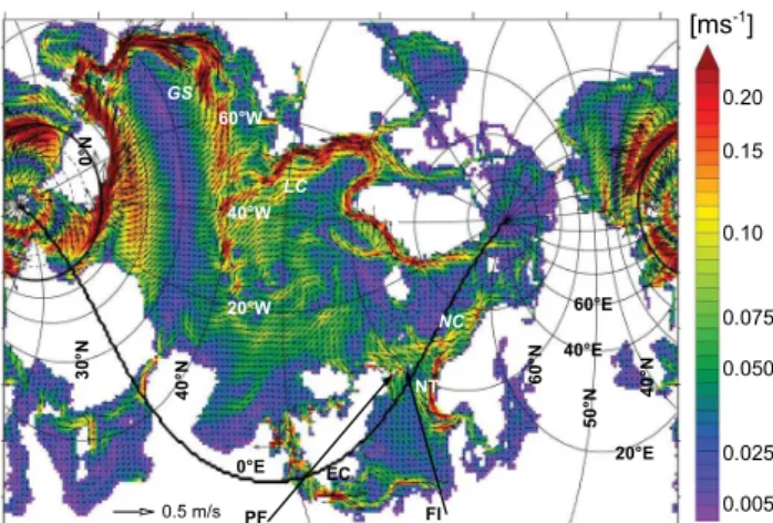
The physical model is the Max Planck Institute for Mete-orology global primitive equation OGCM (MPIOM). It is a z-level model with a free surface. The model assumes the hydrostatic and Boussinesq approximations. It includes a dynamic thermodynamic sea ice model following Hibler (1979). Tracer and momentum advection follows a second-order total variation diminishing scheme after Sweby (1984). The model’s equations are discretized on a bipolar orthogo-nal curvilinear C grid. The water column is subdivided by 30 levels, eight of which lie within the uppermost 100 m. MPIOM includes no explicit turbulence closure. The vertical eddy viscosity and tracer diffusion follows the parameteriza-tion of Pacanowski and Philander (1981, PP hereafter). Since this scheme underestimates mixing close to the surface an ad-ditional parameterization for wind stirring is included (Jung-claus et al., 2006). A detailed model description and valida-tion of physical properties is given in Marsland et al. (2003). For the specific application on the NW European shelf the model’s grid has been set up with a resolution of nominal 1.5◦and the grid poles are placed over central Europe (49◦N, 8◦E) and North America (44◦N, 89◦W) in order to maxi-mize the resolution for the NW European shelf (10 km in the German Bight) and for the adjacent North Atlantic. Figure 1 shows the model domain of the applied grid set-up focus-ing on the NW European shelf/North Atlantic. As the tidal movement is important both, for vertical mixing, and for the transport by the residual currents on continental shelves, the full potential of lunisolar tidal forces is prescribed according to Thomas et al. (2001). The appropriate simulation of tidal effects requires a relatively short time step of 45 min. A de-tailed and comprehensive description of the physical set-up will be given in Sein et al. (2013).
2.2 The carbon cycle and biogeochemistry model
Embedded in the physical model is the biogeochemical mod-ule HAMOCC (HAMburg Ocean Carbon Cycle model, Wet-zel et al., 2005), i.e. it uses the same grid configuration as MPIOM and the advection and diffusion of biogeochemical tracers are identical to temperature and salinity.
Fig. 1.Model domain. The zero meridian is indicated by the thick line. Also shown: surface circulation averaged over 1990–1999. Only every fourth vector is shown. EC is English Channel, NT is Norwegian Trench, PF is Pentland Firth, FI is Faire Island, NC is Norwegian Current, LC is Labrador Current, GS is Gulf Stream.
HAMOCC is a modified nutrient, phytoplankton, zoo-plankton, detritus (NPZD-type) biogeochemistry model. In case of sufficient light, phytoplankton growth is limited by dissolved phosphate (PO4), nitrate (NO3), or iron, which
are fixed into organic soft tissue together with DIC fol-lowing Redfield stoichiometry during photosynthesis. The growth rate is further dependent on water temperature (Ep-pley, 1972). The detritus pool is formed by dead phyto- and zooplankton and fecal pellets. Besides these biomass groups, dissolved organic matter is formed from excretion of liv-ing biomass. All organic matter is remineralized to inorganic constituents by consumption of oxygen or alternatively, by reduction of nitrate (denitrification) or eventually sulphate when not enough oxygen is available. At the sea floor the model is closed by a 12 layer sediment model following Heinze et al. (1999). Within the sediment, organic matter is further decomposed by consuming either oxygen or nitrate. Porewater phosphate, nitrate, and DIC is exchanged with the bottom layer using constant diffusion coefficients. Air–sea gas exchange for oxygen, nitrogen, and carbon dioxide is cal-culated from the local air–sea difference of respective partial pressures according to Wanninkhof (1992) with an improved temperature dependency (Gr¨oger and Mikolajewicz, 2011). A technical model description is provided by Maier-Reimer et al. (2005). A comprehensive and detailed description of the model’s organic and inorganic carbon cycle as well as the included nitrogen and sulphur cycle along with a pro-found validation of global climatologies is given in Ilyina et al. (2013).
We also implemented global riverine inputs of PO4, NO3,
Fig. 2.Prescribed average concentration of riverine nutrient supply to the North Sea. Grey lines indicate monthly mean values. Red line indicates yearly mean values.
the area of interest which is comparable with many regional models (e.g. Moll and Radach, 2003).
In order to improve the model’s performance in simulating the seasonal cycle of nutrients and phytoplankton we had to modify the light penetration scheme of the biogeochemistry model HAMOCC. Details of this light penetration scheme are given in the appendix.
3 Experiments
The model was spun up for several thousand years by forcing the model repeatedly with 6-hourly atmospheric fields taken from the ECHAM5/MPIOM IPCC AR 4 preindustrial con-trol run (Roeckner et al., 2006). For the atmospheric forcing data no bias correction has been applied.
The experiments listed in Table 1 are designed to inves-tigate the effects of climate warming, rising atmospheric
pCO2, and anthropogenic eutrophication separately. For
this, experiments CWE (climate warming effect), CWE-CEE (CWE-carbon emission effect), and CWE-CWE-CEE-AES (CWE-CEE-anthropogenic eutrophication scenario) were started and forced by the atmospheric output from the MPI-ECHAM5 IPCC AR 4 20th century and A1B scenario sim-ulations between 1860 and 2100. In experiment CWE the pure effect of climate warming was tested by keeping the atmosphericpCO2fixed at 288 ppm for the biogeochemistry
model. Experiment CWE-CEE includes also the rise of atmo-sphericpCO2for the biogeochemistry model and run
CWE-CEE-AES includes both, rising atmosphericpCO2 and an
anthropogenic eutrophication scenario for the NW European shelf which today receives riverine nutrients from industrial agriculture. Thus, river concentrations of dissolved phospho-rous and nitrate were exponentially increased between 1860 and 1976 to match observations available between 1976 and 2006 (updated data from Paetsch and Lenhart, 2004, Fig. 2). After 2006, monthly mean values from the last 5 years were repeated until 2100. Thus, there is no trend in riverine nutri-ent supply during the 21st cnutri-entury. We further note that our assumption of riverine eutrophication does not consider the changes during the two world wars. Thus, the period before
1976 is not analysed here. Run CTRL (control integration) continues the spin-up simulation, which allows the separa-tion between real signals and residual model drift.
In addition, two sensitivity experiments were conducted to investigate the efficiency of the carbon shelf pump exem-plary for the North Sea and the adjacent Atlantic (Table 1). In run CO2-NS atmospheric pCO2 was locally set to only
1112 ppm over the North Sea, in order to study the effect on the global carbon cycle. Experiment MARKER was carried out to study the fate of North Sea water after it leaves the North Sea, i.e. does it really reach the deep ocean or does it remain within the ocean’s mixed layer, where it is exposed to the atmosphere and subject to air–sea gas exchange. In en-semble experiment MARKER, 10 model runs were restarted from experiment CWE at the first of July in subsequent years from 1975 to 1984. In these experiments the North Sea water was homogeneously initialized with a tracer concentration of 1, whereas outside the North Sea the tracer was initialized with a concentration of 0. The tracer concentration in subsur-face layers was subject to advection and diffusion only. In the model’s surface layer the tracer concentration was addition-ally altered by a simple air–sea gas exchange using a fixed air tracer concentration of 0 and a characteristic piston ve-locity of 100 m yr−1. The tracer inventory found outside the North Sea is thus an approximate measure for the potential of the North Sea shelf to really enrich the ocean with the tracer. We chose the 1st of July for starting the ensemble members because at this time the water column in the North Sea is strongly stratified. Thus, tracer rich-bottom waters are shel-tered from exposure to the atmosphere at this time and have the highest potential to reach the open ocean.
4 Model performance and validation
Before applying the model to the IPCC A1B climate pro-jection, the model’s performance must be tested for both the global climatology, and the regional climatology in the area of interest in order to determine the extent to which the con-trol period reproduces recent climate/ecosystem conditions. In the following section we validate the results of experiment CWE-CEE-AES as it includes both, the effects of rising at-mosphericpCO2and the anthropogenic eutrophication in the
North Sea. Thus, this set-up is closest to reality. We concen-trate primarily on the modelled distributions of dissolved nu-trients since these variables integrate the different processes related to advection, diffusion, biological consumption and production, decomposition, remineralization, and tempera-ture.
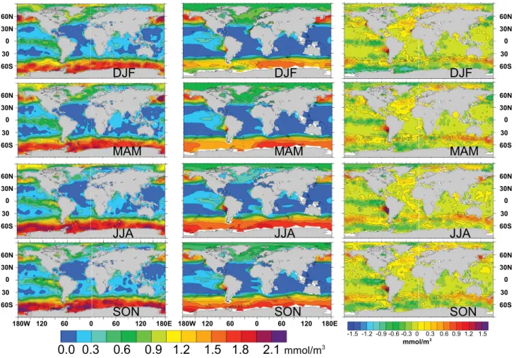
Fig. 3.Seasonal cycle of surface phosphate from observations from the World Ocean Atlas (left, Garcia et al., 2010), compared to model results (average for years 1993–2008, middle column), and modelled minus observed surface phosphate (right).
Table 1.Model experiments. CWE is climate warming effect, CEE is carbon emission effect, AES is anthropogenic eutrophication scenario.
Experiment pCO2 Eutroph. Period
CTRL 288 no without climate warming
1860–2100
CWE 288 no 1860–2100
CWE-CEE 288–700 ppm no 1860–2100
CWE-CEE-AES 288–700 ppm yes 1860–2100
CO2-NS 288 ppm but NS: 1112 ppm no 1980–2000
MARKER 288 ppm no 10 runs of 5 yr integration1
1Ensemble runs were started on 1 July 1975, 1 July 1976, ...1 July 1979.
4.1 Global ocean
The global patterns of dissolved nitrate and phosphate are very similar since HAMOCC models’ biological nutrient up-take strictly according to the Redfield ratio and nitrogen spe-cific processes such as N2fixation and denitrification are tied
to local environments. We here therefore concentrate primar-ily on the modelled distribution of dissolved phosphate. The global distribution of nutrients is similar to the one validated
in Ilyina et al. (2013). Therefore, for nitrate the reader is re-ferred to the paper mentioned above.
Fig. 4.Modelled annual mean distributions for phosphate(a)and nitrate(b)along 35◦W (Atlantic, left) and 180◦E (Pacific, right) compared to observations from the World Ocean Atlas (Garcia et al., 2010).
1993). In these two regions the model clearly underesti-mates phosphate concentrations, which results probably from an overestimation of biological consumption due to a too-weak iron limitation (Ilyina et al., 2013). Enhanced con-centrations are also associated with the wind-driven eastern Pacific equatorial divergence, and the upwelling along the coasts of western Africa and western South America (Maier-Reimer, 1993). The northern North Atlantic is marked by a pronounced seasonal cycle, which is mainly caused by the
nutrient-consuming biological production during spring and summer and nutrient accumulation during winter (Fig. 3). Lowest concentrations are seen in the subtropical gyres which are marked by downward Ekman pumping and a thin mixed layer (Maier-Reimer, 1993; Wetzel, 2004).
The vertical nutrient distributions are shown in Fig. 4. The main deep and intermediate waters can be well recog-nized by their nutrient content. Along the Atlantic section North Atlantic Deep Water (NADW) causes low nutrient concentrations between 1800 and 4000 m water depths. This water mass is formed with a large component of nutrient-depleted surface water originating from the subtropical At-lantic (Broecker and Peng,1982; Maier-Reimer, 1993). The meridional overturning circulation of the model (14 Sv de-picted at 26.5◦N) is in the lower range of published mod-elled values (10 to 20 Sv, e.g. Persechino et al., 2012; Jung-claus et al., 2013) and from a 4-year observational cam-paign (18.7 Sv Kanzow et al., 2010). Below the NADW, Antarctic Bottom Water can be recognized by higher phos-phate concentrations. This is an older, poorly ventilated wa-ter mass which has gained a lot of nutrients by remineral-ization of organic matter (Broecker and Peng, 1982; Maier-Reimer, 1993). In the Southern Ocean at deeper layers the nutrient content is slightly underestimated. Pronounced fea-tures of the Atlantic section are the nutrient rich Antarctic In-termediate Water which gains nutrients by remineralization of organic matter (Maier-Reimer, 1993), and the North At-lantic where nutrient-depleted surface waters are transferred to depth due to deep convection (Maier-Reimer, 1993) and spread southward as NADW. Due to the conveyor belt circu-lation the Pacific ocean is generally nutrient richer compared to the Atlantic (Broecker, 1991). This feature is is well repro-duced by the model. The highest nutrient concentrations are reached in the North Pacific at intermediate depths between 1000 and 2000 m. This is underestimated by the model. In both, the Atlantic and Pacific Ocean, Ekman pumping in the subtropical gyres transfers nutrient depleted surface waters to depths (Maier-Reimer, 1993). In the Pacific, the Southern Hemisphere’s subtropical convergence cell extents deeper than the one in the Northern Hemisphere, which compares well with observations from the WOA. Globally integrated fluxes of CO2, primary production, and export production are
well within the range of published values (Table 3).
4.2 North Sea
Fig. 6. (a)Annual mean of surface temperature (red) and salinity (blue) averaged over the North Sea. Dotted lines indicate the control integration CTRL,(b)annual mean bottom-surface salinity difference averaged over the North Sea,(c)0–100 m (black) and 614–713 m (red) water temperature averaged over the continental slope northwest of the North Sea (12◦W–6◦W; 56◦N–61◦N, indicated by the red box in Fig. 7),(d)same as(c)but for salinity,(e)yearly primary production integrated over the North Sea. Dotted lines indicate the control integration CTRL,(f)carbon absorption of the North Sea (Mt C). Dotted lines indicate the control integration CTRL,(g)winter gross mass transports of nitrate into the North Sea calculated from experiment CWE,(h)same as(g)but for phosphate. Note: hydrographic properties in(a–d)are the same in all scenario experiments.
Table 2.Budgets of absorption (defined as net C flux into the water column in million tons of carbon) and biological production (million tons of carbon) for the North Sea calculated over the last two decades of the 20th and 21st centuries. Numbers in brackets indicate budgets calculated for the entire NW European shelf (all areas between 37◦N and 65◦N adjacent to the North Atlantic and shallower than 200 m). Last two columns indicate the relative change from 1980–1999 to 2080–2099. PP is primary productivity.
Experiment 1980–1999 2080–2099 Relative change (%)
PP Absorption PP Absorption PP Absorption
CWE 31.07 9.3 21.68 7.15 −30.22 −23.11
(84.74) (18.29) (60.81) (16.05) (−28.24) (−12.25)
CWE-CEE 31.66 9.89 21.66 6.53 −31.58 −33.97
(85.76) (21.16) (60.02) (16.61) (−30.01) (−21.50)
CWE-CEE-AES 40.04 11.80 25.82 7.43 −35.51 −37.03
(130.29) (29.52) (79.04) (20.03) (−39.34) (−32.15)
northern boundary and through the English Channel com-pares well with the observation based estimate of Thomas et al. (2005, see Table 3). Likewise, the net mass trans-ports of carbon across the boundaries are in good agreement with observations. With the exception of the net carbon ex-port across the northern boundary, differences between the modelled transports and the observations are clearly smaller than the model’s standard deviation. The modelled absorp-tion of atmospheric carbon amounts to 0.9 Teramol per year (Tmol yr−1). This corresponds to a mean absorption of
1.5 mol c m−2, which is close to the estimate of 1.3 mol c m−2
given by Lorkowski et al. (2012) and the observation based estimate of Thomas et al. (2005) (1.4 mol c m−2).
The model’s annually integrated primary production amounts to 6.5 mol c m−2. This is clearly lower compared to
red box
[m]
a)
b)
green box
c)
[mmol/m3 PO 43-]
[mmol/m3 NO 3-]
Δ ρ Δ ρ
[mmol/m3 PO 43-]
[mmol/m3 NO 3-]
Thomas et al. (2005). NB is northern boundary, EC is English Channel, ATM is atmosphere, P–E is precipitation–evaporation.
Global Other models Model
Primary production (Pg C yr−1) 24–491 54 Export production (Pg C yr−1) 5.0–9.91 7.2 Carbon uptake 1990–1999 (Pg C yr−1) 1.5–2.22 1.55
North Sea Observation Model
VolumeNB(Sv) −0.18 −0.19 (±0.05)
VolumeEC(Sv) 0.15 0.17 (±0.04)
P-E (Sv) −0.02 (±0.004)
CarbonNB(Tmol yr−1) −13.3 −9.9 (±3.1)
CarbonEC(Tmol yr−1) 10.7 9.0 (±3.9)
CarbonATM(Tmol yr−1) 0.8 0.9 (±0.008)
1Steinacher et al. (2010). 2Orr et al. (2001).
Table 4.Statistics for a quantitative comparison of simulated and observed state variables derived from Taylor diagrams (Taylor, 2001). rms is root mean squared, corr is Pearson’s correlation, stddev is standard deviation, N is number of observations. The statistics have been derived from all 155 boxes shown in Fig. 5. See text for details about data set and data handling.
State variable rms corr stddev observation stddev simulation N
Phosphate 0.25 0.58 0.29 0.24 3529
Nitrate 6.10 0.43 6.00 5.50 2536
Temperature 1.20 0.94 3.40 2.90 5537
Salinity 0.75 0.76 1.10 1.10 5740
4.2.1 Quantitative results
In the following we validate the model’s spatial and tempo-ral variability of temperature, salinity and dissolved nitrate and phosphate. For this we use observational data derived from the Marine Environmental Data Base (MUDAB) and the CANOBA (carbon and nutrient cycling in the North Sea and the Baltic Sea) data set.
MUDAB is a joint project of the Federal Maritime and Hydrographic Agency (BSH) in Hamburg and of the Federal Environmental Agency (UBA) in Berlin. It is managed by the German Oceanographic Data Cen-ter (www.bsh.de/en/marine data/environmental protection/ mudab database/). CANOBA is a data set of carbon and nu-trient measurements on a regular 1◦×1◦station grid for all four seasons between 2001–2002 (Thomas, 2002; Thomas et al., 2004) and additional data from other years.
We here validate a historical experiment. Therefore, in contrast to hindcast simulations forced by reanalysis data, we cannot compare individual years between observed and simulated quantities. The ECHAM atmosphere model used for forcing has its own short-term oscillations (such as the North Atlantic Oscillation) which are realistic by means of amplitudes and frequencies. However, they cannot be
ex-pected to be in phase with reanalysis data that assimilated ob-servations. Therefore, for the following quantitative valida-tion we consider here salinity, temperature, and nutrient data for the period 1993–2008. For this period all available mea-surements for temperature (n=5537), salinity (n=5740),
phosphate (n=3529), and nitrate (n=2536) were used. For
the analysis, the North Sea was subdivided into single boxes of 1◦×1◦extension. Where appropriate, boxes were further
subdivided for depths deeper and shallower than 30 m result-ing in a total number of 155 boxes.
Fig. 8. (a)and(b)average winter (DJF) mixed layer depth at the end of the 20th and 21st centuries.(c)and(d)same as(a)and(b) but for average dissolved surface phosphate concentration.(e)and (f)same as (a)and (b)but for vertically integrated yearly mean primary production.
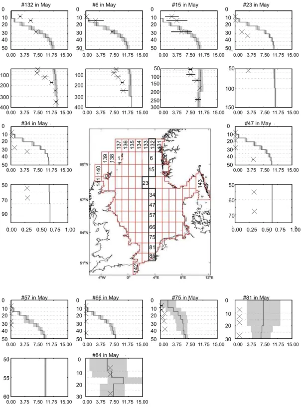
from shallow waters off the Rhine river to the boundary with the North Atlantic near the Norwegian trench. For this, we re-stricted the comparison to available data for winter-, spring-, and summer-representing conditions before, during, and af-ter the spring bloom. Depending on the availability of ob-servations we use either February or March data (winter), or July or August data (summer) for comparison of observa-tions and modelled data in the respective boxes. The results are presented as mean profiles for the respective months in Fig. 5fa–f for phosphate and nitrate. In addition, winter and summer mean profiles for temperature and salinity are pro-vided in the Supplement S2. Further details on the observa-tional data sets and quantitative methods are given in Große and Moll (2011).
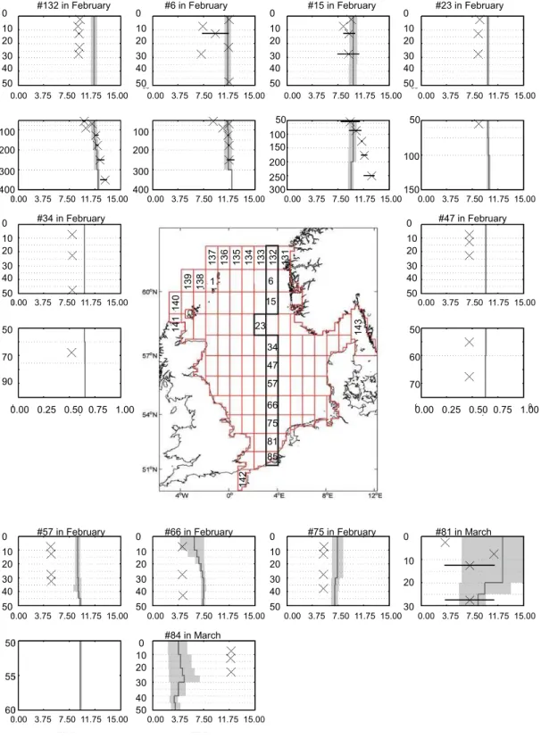
4.2.2 February
The winter situation is characterized by well-mixed condi-tions along the entire transect resulting in overall low verti-cal gradients seen in temperature, salinity, and nutrient con-centrations (Supplement S2, Fig. 5fa, d). The model tends to slightly underestimate phosphate concentrations in the north-ern boxes (132, 6, 15, 23, 34). Further south, the deviation from observations is more pronounced, which is probably linked to the uncertainty in applied river runoff that was cal-culated from the atmospheric forcing fields which cannot be expected to be in phase with observed data.
Nitrate concentrations are generally too high except for the deeper boxes (Fig. 5fd) below 50 m where they fit well with or even slightly exceed observations. Observed and modelled data are most congruent for salinity and temperature where the modelled values are mostly within the range of obser-vations (indicated by the 17 and 83 % percentiles). In most boxes the temperature is slightly too low (Supplement).
4.2.3 May
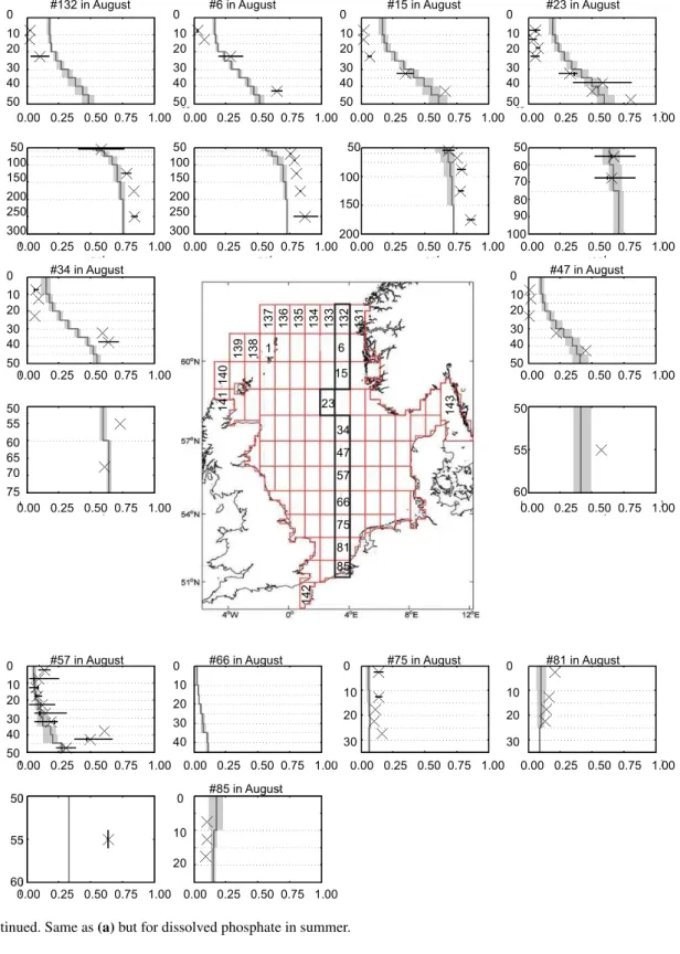
In the northern North Sea both phosphate, and nitrate concen-trations are substantially diminished in the upper 50 m com-pared to the winter situation (Fig. 5fb, e). Below the euphotic zone the changes are less pronounced and nitrate concentra-tions are even substantially higher than in winter. This pattern clearly reflects the spring bloom in the euphotic zone and the onset of stratified conditions in the northern North Sea and is well reproduced in the simulation. In the central North Sea (boxes 57, 66, and 75) the modelled phosphate and ni-trate concentrations are different. While simulated phosphate shows in agreement with observations, very-low to zero gra-dients (except box 66 which has a very large range), simu-lated nitrate is nearly depleted near the surface but exhibits (contrary to observations), still, winter concentrations at 40 to 50 m depth (Fig. 5fe). This may reflect the fact that nitrate is already limiting production at the surface in the simulation and the model’s subsurface production is too weak. Observed nitrate concentrations are close to zero (while phosphate is concentrations are relatively high), which indicates that ni-trate is a nutrient limiting factor. In the southernmost boxes 81 and 85 the water column is well mixed in agreement with observations (Fig. 5fe). Modelled concentrations are clearly too high in box 81 but match well in box 85.
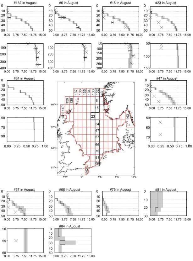
4.2.4 August
Fig. 9. (a)Sea–air carbon flux in experiment CO2-NS. A 10 yr average of 1990–1999 is shown. Positive flux indicates degassing.(b)Relative
change of dissolved inorganic carbon at 95 m depth between experiments CO2-NS minus experiment CWE. Positive values indicate higher
concentrations in experiment CO2-NS. An average over the years 1995–1999 is shown.
0
250 500 750 1000 1250 1500 1750 2000
0 10000 20000 30000 [km3]
Days after model start
Fig. 10. Inventory of marked North Sea water in experiment MARKER. An average over all ensemble members is shown. The red line indicates the total ocean inventory. The blue line indicates open ocean inventory without the North Sea and green line indi-cates the deep ocean inventory below 1000 m water depth. The inter-ensemble variability is very low compared to the mean signal.
model reproduces vertical mean gradients seen in observa-tions in most cases. However, the variability is clearly under-estimated. In the southern North Sea modelled mean values are too low.
The nutrient profiles reflect the stratified conditions with widespread depletion near the surface and high concentra-tions below the euphotic zone. Below the euphotic zone concentrations do not differ much from the winter situation (Fig. 5fc, e). The model performs better for phosphate con-centration. In case of nitrate it overestimates the concentra-tions in boxes 15, 23, 47, and 57. In the northernmost boxes nitrate concentrations fit well with observations.
4.2.5 Overall performance
We showed that the model reproduces fairly well the hydro-graphic and biogeochemical conditions before, during, and after the spring bloom. Thus, the main physical and biogeo-chemical processes, i.e. summer stratification, winter deep mixing and biological consumption, that are characteristic for the North Sea are sufficiently covered by the model es-pecially in the northern North Sea, which is the key region for the exchange with the open NE Atlantic. Near the coasts the model bias for nitrate and salinity is larger, which is most likely related to the uncertainties in the prescribed river runoff calculated from the atmospheric forcing fields.
To roughly asses the overall model’s performance we com-pare physical parameters and nutrients by means of root mean squared error, standard deviation and Pearson’s corre-lation. These parameters are calculated using data from all 155 boxes. The results are summarized in Table 4.
!
"
#
$
"
#
$
$$""$ %&
'('''))))"))# '('''))))"))#
!
*
+$++$+"+"$++$+#+#$+$+$$+, +$++$+"+"$++$+#+#$+$+$$+,
Fig. 11. (a)Available photosynthetic active short-wave radiation averaged over the North Sea south of 54◦N using standard light scheme.(b) Seasonal cycles of phytoplankton (inP units) concentration using standard light scheme.(c)and(d)same as(a)and(b)but using modified light scheme.
and biogeochemistry. Thus, we consider it to be adequate for addressing the questions on which this paper focuses.
5 Climate change during the 21st century
5.1 Stratification on the shelf and along the shelf break
The NW European shelf warms between 1.6 K in off-shore areas and 3.2 K near the coasts in response to the IPCC ARC4 A1B warming scenario. In the North Sea the annually av-eraged surface temperature increases by nearly 2 K in the course of the 21st century (Fig. 6a). This is somewhat lower than the model’s global average warming of 2.5 K. The atmo-spheric forcing is also marked by an intensifying hydrologi-cal cycle, which leads to enhanced moisture transports from the tropics to high latitudes. This intensification of the hydro-logical cycle is seen in most global warming scenarios (Allen and Ingram, 2002; Heldt and Soden, 2006; Mikolajewicz et al., 2007; Wentz et al., 2007). Thus, the global atmospheric pattern of evaporation minus precipitation is enhanced by in-creased surface fluxes. Due to this, most models predict a substantial freshening of the North Atlantic under climate warming. Additional evidence for an ongoing freshening has been/is also supported by observations (Durack et al., 2012). North of 40◦N the entire Atlantic freshens considerably in our simulation (not shown). The North Sea as a shelf basin which is widely surrounded by land is also strongly affected by continental runoff. The enhanced river runoff results in a considerably stronger freshening in comparison with the
open Atlantic and the sea surface salinity decreases by 0.75 in the North Sea (Fig. 6a) at the end of the 21st century. The freshening of the bottom layer is weaker than at the sur-face since the North Sea still receives saltier waters from the adjacent North Atlantic. Accordingly, the bottom to surface salinity difference increases by 0.1 (or 25 %) (Fig. 6b) in the course of the 21st century. The shelf, thus, undergoes consid-erably enhanced stratification.
The stratification is accompanied by a strong decline of nutrient transports from the Atlantic into the North Sea dur-ing the second half of the 21st century (Fig. 6g, h). The nu-trient supply take places mainly during winter when vertical mixing is strongest throughout the year and nutrients are not consumed by biological activity due to limitation of biolog-ical production by light. In all climate change experiments the transport of dissolved phosphate and nitrate at the north-ern boundary of the North Sea is nearly halved (Fig. 6g, h) compared to preindustrial levels.
The decline in winter nutrient supply in the second half of the 21st century (Fig. 6g, h) is not caused by a weaker in-flow of Atlantic water masses northeast of Scotland. Instead, Atlantic water masses entering the North Sea have lower trient concentrations compared to the 20th century. This nu-trient depletion is caused by weaker vertical mixing along the shelf break and the continental slope which, in turn, is caused by hydrographic changes.
Northeast of the North Sea the surface waters become fresher and warmer (red box in Fig. 7b). The surface freshening is seen in the entire Atlantic north of 40◦N (not shown). Further south, in the subtropics (not shown), salinities show over-all positive anomalies in the upper few hundred metres. Be-cause of this, subsurface waters from the subtropics, which are advected northward via the North Atlantic drift, become warmer and saltier, which causes higher salinities and tem-peratures at a depth of approximately 500 m in the region in-dicated by the red box (Fig. 7b). The changes in salinity and temperature result in an enhanced vertical density gradient within the upper 1000 metres (red box in Fig. 7b). The layer to layer gradients of potential density are overall increased in the upper 1000 m (Fig. 7b, lower panel middle plot) which weakens effectively the upward volume transport (Fig. 7b, lower panel left hand) which, in turn, lowers nutrient con-centrations in the euphotic zone (Fig. 7b, lower panel right hand).
Directly north of the North Sea (green box) the hydro-graphic changes in the surface properties are similar to those described for the red box (Fig. 7c). The pycnocline at around 600 m strengthens. The profound decline in surface nutri-ent concnutri-entrations cannot be directly attributed to changes in the mean upward transport at deeper levels. As for this re-gion upward and downward transports are roughly balanced in the upper 500 m, we have to note that the gross up- and downward transports do not change as well at the end of the 21st century. However, between 100 and 400 m the turbulent vertical mixing (not shown) is nearly halved, which indicates a weakening of tidally induced mixing. Of course, part of the nutrient depletion is advected from the adjacent NE Atlantic which is affected by a widespread thinning of the mixed layer (Fig. 8a, b).
The temporal evolution of hydrographic changes is shown in (Fig. 6c, d). Here we compare the upper 100 m of the water column with water from intermediate depth between 810 and 1060 m. For the red box the upper 100 m of the Atlantic has warmed by 1.5 K and freshened by 0.25 per mille at the end of the 21st century, whereas at intermedi-ate depths only slight changes of temperature and salinity are seen (Fig. 6c, d). As a result of this enhanced stability of the water column, the mixing along the shelf break and in the neighbouring NE Atlantic reduces. Accordingly, the winter mixed-layer depth shallows by up to several hundred metres along the shelf break (Fig. 8a, b). As a result, the up-ward mixing of nutrient-rich waters from below the photic zone to shallower water depths is essentially reduced. These wide areas of the NW European shelf have been virtually cut off from the mid-depth Atlantic nutrient source. As a result, the on-shelf nutrient supply from the Atlantic breaks down and the nutrient inventory of the North Sea diminishes. In the northern North Sea the nutrient concentrations are low-ered locally by up to 50 % compared to the end of the 20th century (Fig. 8c, d), which has widespread negative effect on primary production (Fig. 8e, f). The lowered nutrient
concen-trations are clearly the result of lowered imports from the NE Atlantic because no significant changes in the winter mixed-layer depth are seen in the North Sea. The southern North Sea is less affected as the nutrient-rich water masses from the north are usually diverted eastward when they reach the central North Sea. Here, nutrient concentrations are reduced due to the prescribed strong reduction of riverine phosphate inputs in the early 1990s.
5.2 Decline in biological productivity
Due to the reduced winter nutrient import from the Atlantic, which is caused by the stronger stratification, the nutrient in-ventory of the North Sea diminishes by 33 % at the end of the 21st century in the experiments without anthropogenic eutrophication, CWE and CWE-CEE. This results in lower biological production in the North Sea, which is reduced by
∼31 % in experiments CWE and CWE-CEE from the last two decades of the 20th century to end of the 21st century (Fig. 6e, Table 2). The reduction of North Sea productiv-ity is of similar magnitude as for the entire NW European shelf, where the reduction varies between 30 and 39 % in the respective experiments (Table 2). Remarkably, the pro-ductivity decline on the shelf is much stronger than in the open ocean. For the open North Atlantic and the global ocean our model predicts a productivity reduction of only 17 and 15 %, respectively, which agrees well with results from other models which predict reductions between 2 and 20 % result-ing from stronger open ocean stratification (Steinacher et al., 2010). We thus conclude that the NW European shelf pro-ductivity is much more vulnerable to climate warming than the open ocean in our model. The higher vulnerability arises from the above described stratification feedback along the shelf which acts in addition to the well-known stratification impact on marine productivity in the open ocean (Steinacher et al., 2010). Due to the area-wide nutrient depletion, produc-tion lowers likewise in the adjacent NE Atlantic (Fig. 8e, f). Enhanced production is seen only in regions suffering from reduced sea ice coverage, which promotes a longer growing season. However this effect becomes important only in the Arctic Ocean where productivity increases substantially.
century in experiment CWE-CEE-AES. In this experiment the stratification feedback along the shelf edge leads to a de-cline of North Sea productivity in the course of the 21st cen-tury as well (Fig. 6e). Here, uncertainties are associated with the chosen scenario for 21st century nutrient discharges.
5.3 Impact of risingpCO−2 and declining productivity
on carbon absorption
Consistent with many studies based on observations (e.g. Frankignoulle and Borges, 2001; Thomas et al., 2005) our simulations show that the North Sea is a sink for atmo-spheric CO2. The yearly integrated carbon absorption varied
between 9.3 and 11.8 million tons of carbon (Mt C, here-after) in the last two decades of the 20th century (Table 2) in agreement with published values based on observations (9.5 Mt C, Thomas et al., 2005). Interestingly, the rising at-mospheric pCO2 in experiment CWE-CEE has nearly no
effect on carbon absorption in the North Sea (Fig. 6f, blue line). In this experiment carbon absorption is hardly higher than in experiment CWE without rising atmosphericpCO2.
As the air–sea exchange for CO2can be characterized –
in-cluding the buffering of the carbonate system – by a piston velocity of 100 m yr−1, the North Sea is almost in equilib-rium with rising atmospheric levels of CO2. In experiment
CWE-CEE carbon absorption in the last two decades of the 20th century is higher only by 0.59 Mt C (=6.3 %) than in
experiment CWE (Table 2) although the atmosphericpCO2
has risen by 22 %. At the end of the integrations carbon ab-sorption in experiment CWE is even higher than in CWE-CEE although the atmosphericpCO2 was kept fixed at the
preindustrial level in run CWE. In all experiments, the At-lantic water masses entering the North Sea decrease in DIC because the rising water temperatures lower the solubility of CO2and enhanced stratification reduces the upward mixing
of DIC-rich water masses from the deep Atlantic. This lowers the DIC imports from the Atlantic which, in turn, will lower the local waterpCO2in the North Sea and thus enhance
car-bon absorption. In experiments CWE-CEE and CWE-CEE-AES, however, the DIC decrease in the adjacent Atlantic is relatively small compared to experiment CEE as the upper-oceanpCO2in the former two experiments adapts rapidly to
the rising atmosphericpCO2.
Changes in biological productivity have a stronger impact on carbon absorption of the North Sea than the rising at-mosphericpCO2. Thus, in experiment CWE-CEE-AES
ab-sorption is enhanced by about 25 % between 1975 and 1985 compared to run CWE-CEE (Fig. 6f). In all experiments the decreasing biological productivity in the course of the 21st century strongly reduces atmospheric carbon absorption (Fig. 6f). The relative reductions in carbon absorption range between 23 and 37 % for the North Sea and 12 and 32 % for the entire NW European shelf (Table 2). The strongest decline is simulated in experiment CWE-CEE-AES (37 % in the North Sea) which likewise exhibits the strongest
de-cline in productivity. Part of this decrease is a direct conse-quence of the assumed reduction in anthropogenic eutroph-ication. However, in the experiment CWE-CEE without an-thropogenic nutrient input, the net uptake of anan-thropogenic CO2is still reduced by 34 %.
6 Does continental shelf pumping really enhance the oceanic storage of carbon?
Strong absorption on the shelf does not necessarily result in long-term oceanic carbon sequestration since a large portion of the shelf water exported to the open ocean remains within the mixed layer and does not reach the deep ocean. In the following we describe two experiments that were designed to estimate how much anthropogenic carbon absorbed in the North Sea has the potential for long-term sequestration.
6.1 Experiment CO2-NS
In experiment CO2-NS we repeated the period 1980–2000
from experiment CWE (Table 1) but fixed the atmospheric
pCO2to 1112 ppm over the North Sea whereas for the rest
of the ocean the atmosphericpCO2is as in experiment CWE
(Table 1). As expected, experiment CO2-NS is marked by
im-mediately high carbon fluxes into the North Sea in response to the sudden increase of atmosphericpCO2. After the
ini-tial adaptation period of about 2 months only those areas are marked by strong carbon absorption where lowpCO2waters
from outside enter the North Sea (Fig. 9a) like in the English Channel and east of Scotland. Waters leaving the North Sea via the Norwegian coastal current are marked by vigorous degassing. Along the pathway of North Sea water a plume of pronounced DIC enrichment is visible (Fig. 9b). Most of this water enters the Barents Sea via the Norwegian Current at a core depth of around 100 m. There is no significant portion that reaches directly the deep convection sites in the Green-land Sea.
Already after 20 yr of integration the air–sea carbon fluxes are in equilibrium and show no significant trend in exper-iment CO2-NS. In experiment CO2-NS the North Sea still
absorbs 6.03 Mt C month−1 more compared to experiment CWE. If all of the carbon absorbed over the North Sea would be sequestered in the deep open ocean, then the globally in-tegrated oceanic carbon uptake should be enhanced by the same amount.
However, the global ocean uptake rises by only 1.2 Mt C month−1 along the Norwegian Current (Fig. 9a).
to find out whether or not the carbon shelf pumping is also very vulnerable to the climate warming in the course of the 21st century. From this experiment we calculate that at the end of the 21st century only 13.6 % of carbon absorbed over the North Sea is being stored longer in the open ocean. This means that the efficiency of carbon shelf pumping is also de-creasing in case of climate warming.
6.2 Experiment MARKER
In order to explain the mechanism behind the low effi-ciency of the carbon shelf pump, we carried out experi-ment MARKER (Table 1). This experiexperi-ment was designed to quantify the amount of North Sea water that reaches the open ocean without undergoing intense modification by air– sea gas exchange. For this, we marked the North Sea water stock with an artificial tracer (see Sect. 3) and integrated the model for four years. From the resulting tracer distribution we calculated the volume of water originating from the North Sea in the open ocean. We note that the uniform initialization of the tracers in the North Sea in this experiment differs from realistic conditions, since tracers (such as, e.g. DIC) are usu-ally higher concentrated below the pycnocline during sum-mer. Hence, the cross-pycnocline gradients in the northern North Sea are likely a bit too low during the first few weeks of the experiment. However, since the adaption time of the water layers above the pycnocline to the atmospheric bound-ary layer due to air–sea gas exchange is much faster than the turbulent mixing across the pycnocline in the water column, we do not believe this has significant influence on the calcu-lated tracer export to the open ocean.
The results of experiment MARKER show that already within the first year the marked North Sea water stock is re-duced to less than 15 % of the initial volume of 37 494 km3 (Fig. 10, red line). After this steep decline the marked North Sea water stock is further reduced at low rates between 2 and 3 km3d−1. With the beginning of the next cold sea-son (after abount 500 days of integration) the mixed layer thickens again which results in slightly enhanced decompo-sition rates in the range of 10 to 15 km3d−1. After four years a stock of only 955 km3 (2.6 % of the initial stock) exists which is decomposed at rates between 0.2 km3d−1in sum-mer and 0.7 km3d−1 in winter. About 98 % of this stock is located outside the North Sea in the open ocean (Fig. 10c, blue line). However, at the end of experiment MARKER only 188 km3are stored at depths below 1000 m (Fig. 10, green line) though this stock still is slightly growing at a rate of ap-proximately 0.1 km3yr−1. In conclusion, the rapid
decompo-sition of the North Sea stock as well as the very low amount of North Sea water stored at depths below 1000 m clearly in-dicates that most of the water exported from the North Sea remains in the ocean’s mixed layer, where it is still exposed to the atmosphere.
7 Discussion of model results and potential uncertainties
Since our biogeochemistry model was originally designed for the open ocean, it includes some simplifications com-pared to regional models and may lack important processes which may become important for biological production in the shelf environment. This imposes some uncertainties on the model’s results on productivity and carbon absorption. In the following, we address the uncertainties associated with the model and experimental set-up.
7.1 Biological production
Our model predicts a substantial weakening of primary pro-duction and carbon absorption for the NW European shelf. These changes are caused by a widespread thinning of the mixed layer along the shelfbreak and the adjacent continen-tal slope in the NE Atlantic which diminishes the on-shelf nutrient transport. This raises two questions: how robust are the results with regard to the fact that we have used only one specific warming scenario and forced our model with the output from only one atmospheric model? To address these questions we evaluated the response of the North At-lantic mixed layer in available scenario simulations carried out in the frame of the Max Planck Institute’s contribution to the Climate Model Intercomparison Project (CMIP5). In particular we compare the historical experiments for the 20th century with the representative concentration pathway (RCP) warming scenarios 4.5 and 8.5. All model runs were con-ducted using the state of the art coupled atmosphere–ocean GCM ECHAM6/MPIOM/HAMOCC (MPI-ESM) with two different model resolutions (Jungclaus et al., 2013). The sce-narios were carried out in ensembles of respectively three re-alizations, each of them initialized from three different restart files of the preindustrial control run (see Giorgetta et al., 2013 for details).
Indeed, all four state-of-the-art coupled atmosphere–ocean– ecosystem models applied in this study showed the charac-teristic increase in stratification together with a profound de-cline in productivity. From this we conclude that the strati-fication feedback is not a phenomenon specific only to our model, but is a rather characteristic feature of warming sce-narios seen in most coupled climate models.
Our finding of reduced on-shelf nutrient transports is in good agreement with recent modelling results of Holt et al. (2012) who found a reduction of nitrogen transports onto the NW European shelf by 20 % at the end of the 21st cen-tury. However, in their model they found only a small effect on primary production which decreased by only 5 % on av-erage. In fact the authors found several temperature related effects stimulating production. However, the temperature ef-fect on biological production is very complex as it influences a number of biological processes with opposing effects on production such as the remineralization of organic matter, the growth and mortality rates of phytoplankton and zooplank-ton, etc. Therefore the response of biological production to elevated temperatures is subject to considerable uncertainty. We note that our model’s organic matter remineralization is not temperature dependent, and thus it lacks the potential positive effect of enhanced nutrient recycling on biological production. Therefore, the strong decline in production pre-dicted by our model may be slightly overestimated.
7.2 Carbon absorption and shelf pumping
Our results agree with observational and modelling studies indicating the NW European shelf and the North Sea in par-ticular a net sink for atmospheric carbon (e.g. Frankignoulle et al., 2001; Bozec et al., 2005; Thomas et al., 2005; Borges et al., 2006; Prowe et al., 2009; K¨uhn et al., 2010’ Lorkowski et al., 2012). Based on extensive observational campaigns in the North Sea Thomas et al. (2004) could show that much of the carbon absorbed reaches the open NE Atlantic. This agrees with tracer experiments indicating that 40 % of car-bon sequestered in the North Sea is exported to the NE At-lantic (Holt et al., 2009). However, only about 50% of this are injected at below the pycnocline (Wakelin, et al., 2012) yielding an efficiency for the carbon shelf pump of 20%. This agrees very well with our estimation of likewise 20% effi-ciency. In our model, much of the carbon exported to the open ocean through the Norwegian trench gets exposed to the atmosphere when it joins the Norwegian Current north of 60◦N (Fig. 9). Here, the water column’s stabilizing influ-ence of the fresher surface waters originating from the Baltic Sea, which predominates along the Norwegian coast to the North Sea, gradually ceases due to mixing with higher saline Atlantic waters within the Norwegian Current. This region is not included in most regional model set-ups (e.g. Prowe et al.; 2009, Holt et al., 2012; Wakelin et al., 2012; Lorkowski et al., 2012). The region directly north of the North Sea is of minor importance in this respect.
An early attempt to asses the efficiency of the carbon shelf pump was undertaken by Yool and Fasham (2001). The au-thors used a global physical ocean GCM and implemented DIC and dissolved organic carbon (DOC) as passive tracers. Using a simple piston velocity for air–sea gas exchange they found the North Sea carbon pump to be 30 % efficient, which is somewhat higher than estimated by Wakelin et al. (2012) and our study. Within the world’s shelf area the North Sea efficiency appears low (ranked as 25 out of 32 shelf seas in Yool and Fasham, 2001). On the other hand, the strength of shelf pump is not only determined by its efficiency to ex-port carbon to subpycnocline depths but also by the uptake of atmospheric carbon which is on the NW European shelf largely driven by biological processes (e.g. Gypens et al., 2004; Huthnance et al., 2009; Lorkowski et al., 2012).
8 Summary and conclusions
Here we have shown results from a novel approach to simu-late biogeochemical changes on the NW European shelf with a global model with enhanced resolution on the NW Euro-pean shelf. This approach avoids the problem of prescrib-ing boundary conditions in the interior of the ocean for dy-namical downscaling simulations of anthropogenic climate change.
Most global models (Steinacher et al., 2010) predict a de-crease between 2 and 20 % in open ocean productivity in re-sponse to climate warming. We have shown that on the NW European shelf the relative reduction in productivity is much stronger due to the suppression of lateral nutrient input re-sulting from the weakening of vertical mixing along the shelf break. This process is essential for both the nutrient supply to the outer shelf and productivity, and can be considered as most vulnerable under climate warming. In case of the North Sea the nutrient transport from the deep Atlantic declines by up to∼50 % in the 21st century and productivity decreases
by∼35 % assuming current rates of anthropogenic nutrient
eutrophication. Even if we neglect anthropogenic eutrophi-cation in our simulations (experiments CWE and CEE) the shelf productivity is reduced by about∼30 % in the North
Sea and on the entire NW European shelf (Table 2). This is twice as strong as the reduction in open ocean productivity.
A decline of North Atlantic primary production over the last century has been already reported by Boyce et al. (2010). Shelf productivity has been assumed to be stable or rather to increase with an intensification of river runoff (Boyce et al., 2010), thus providing rather stable conditions for the eco-logical food web and for fisheries. This study provides a first hint that also the on-shelf ecological food web could be threatened by global warming. However, more modelling ef-forts involving a broader range of tested scenarios and atmo-spheric models are necessary.