Artificial neural network for prediction of the area under the disease progress curve

(1)

ABSTRACT: Artificial neural networks (ANN) are computational models inspired by the neural systems of living beings capable of learning from examples and using them to solve problems such as non-linear prediction, and pattern recognition, in addition to several other applications. In this study, ANN were used to predict the value of the area under the disease progress curve (AUDPC) for the tomato late blight pathosystem. The AUDPC is widely used by epidemiologic studies of polycyclic diseases, especially those regarding quantitative resistance of genotypes. However, a series of six evaluations over time is necessary to obtain the final area value for this pathosystem. This study aimed to investigate the utilization of ANN to construct an AUDPC in the tomato late blight pathosystem, using a reduced number of severity evaluations. For this, four in-dependent experiments were performed giving a total of 1836 plants infected with Phytophthora infestans pathogen. They were assessed every three days, comprised six opportunities and AUDPC calculations were performed by the conventional method. After the ANN were created it was possible to predict the AUDPC with correlations of 0.97 and 0.84 when compared to con-ventional methods, using 50 % and 67 % of the genotype evaluations, respectively. When using the ANN created in an experiment to predict the AUDPC of the other experiments the average correlation was 0.94, with two evaluations, 0.96, with three evaluations, between the predicted values of the ANN and they were observed in six evaluations. We present in this study a new paradigm for the use of AUDPC information in tomato experiments faced with P. infestans. This new proposed paradigm might be adapted to different pathosystems.

Keywords: Phytophthora infestans, ANN, AUDPC, artificial intelligence, plant breeding 1_{Santa Catarina State Agricultural Research and Rural}

Extension Agency − Experimental station of Ituporanga, Estr. Geral Lageado Águas Negras, 453 − 88400-000 − Ituporanga, SC − Brazil.

2_{São Paulo State University/College of Technology and} Agricultural Sciences, Rod. Cmte João Ribeiro de Barros, km 65 − 17900-000 − Dracena, SP − Brazil.

3_{Federal University of Viçosa − Dept. of Phytotechny, Av.} Peter Henry Rolfs, s/n − 36570-000 − Viçosa, MG − Brazil. 4_{Federal University of Viçosa − Dept. of Animal Science.} 5_{Federal University of Viçosa − Dept. of General Biology.} *Corresponding author <danielalves@epagri.sc.gov.br>

Edited by: Luís Eduardo Aranha Camargo

Artificial neural network for prediction of the area under the disease progress curve

Daniel Pedrosa Alves1_{*, Rafael Simões Tomaz}2_{, Bruno Soares Laurindo}3_{, Renata Dias Freitas Laurindo}3_{, Fabyano Fonseca e} Silva4_{, Cosme Damião Cruz}5_{, Carlos Nick}3_{, Derly José Henriques da Silva}3

Received July 31, 2015 Accepted March 19, 2016

Introduction

Tomato late blight, caused by Phytophthora infes-tans (Mont.) de Bary, can cause complete loss if it is not properly controlled, and has been considered one of the most devastating tomato diseases worldwide (Irzhansky and Cohen, 2006). Nowicki et al. (2012) reported yield losses of up to 100 % caused by the pathogen. Genetic resistance is considered the most efficient method for controling plant pathogens, since it reduces production costs, facilitates disease man-agement, and does not have the impacts produced by fungicides.

The area under the disease progress curve (AUD-PC) is a valuable tool for measuring harvest losses due to pathogen attack (Ferrandino and Elmer, 1992) and in epidemiological studies of polycyclic diseases, especial-ly those regarding quantitative resistance studies (Jeger and Viljanen-Rollinson, 2001). The conventional esti-mator of AUDPC is the equation developed by Shaner and Finney (1977), which considers the information of multiple severity evaluations, and yields a single value. Jeger and Viljanen-Rollinson (2001) proposed a method for calculating the AUDPC with only two evaluations for the wheat pathosystem – Puccinia striiformis f. sp. tritici, which was later validated by Mukherjee et al. (2010) for the rice pathosystem –

Pyricularia grisea. Nonetheless, Jeger and

Viljanen-Rollinson (2001) reinforce that the methodology has three assumptions that should be satisfied: first, the resistance must be expressed as the disease rate and not as the absence of symptoms; second, the disease evaluated has to be present in all plants during the same timeframe; and third, the disease progress has to be continuous. These assumptions make the appli-cation of this method to the tomato pathosystem diffi-cult - Phytophthora infestans. Thus, the artificial neural network (ANN) methodology stands out because it is based on machine learning, regardless of the model, with wide application in agricultural sciences.

ANN are defined as non-algorithmic computa-tions characterized by systems that, at a certain level, resemble the structure of the human brain (Braga et al., 2000). In practice, they constitute data modeling tools (Goyal, 2013). This methodology has been wide-ly used in agriculture, and it can go beyond human capacity to evaluate large data banks and relate them to a specific desirable characteristic. ANN have been used in simulation studies to predict genetic values (Silva et al., 2014; Peixoto et al., 2015), and in associa-tion with genomic analysis (Gianola et al., 2011; Ehret et al., 2015).

This study aimed to investigate the prediction ca-pacity of ANN to obtain AUDPC values for tomato late blight using a lower number of evaluations to improve the process efficiency.

(2)

Materials and Methods

Plant material, inoculation, and assessment

Experiments were performed in Viçosa, MG − Brazil (20°45’14” S and 42°52’53” W, altitude of 648.74 m). According to Köppen’s classification, the climate is Cwa, average relative humidity of 80 %, average yearly maximum and minimum temperatures of 26.4 and 14.8 °C, respectively, and average yearly rainfall of 1.221.4 mm. Late-blight resistance was assessed in 192 tomato (Solanum lycopersicum) accessions (Table 1) from the Germplasm Bank of the Universidade Federal de Viçosa (BGH-UFV) in the field.

Accessions were evaluated in four experiments in a randomized block design with three replications and three plants per plot. Experiment 1 was performed from Jan to May 2009, consisting of 53 accessions; Experiment 2 from Apr to Aug 2009, consisting of 47 accessions; Ex-periment 3 from Feb to May 2010, consisting of 52 acces-sions; and Experiment 4, from Mar to July 2010, with 52 accessions (Table 1). The cultivars Santa Clara, Deborah, and Fanny were adopted as a susceptibility pattern in each experiment.

Plants were inoculated with a mix of sporangia originating from different P. infestans strains collected from different regions of Brazil, 45 days after plant-ing, according to Abreu et al. (2008). Disease sever-ity evaluations were made following the diagrammatic scale proposed by Corrêa et al. (2009), and were started 3 days after inoculation at regular intervals of 3 days, totaling five evaluations (day 3, 6, 9, 12 and 15 after in-oculation, DAI – evaluations 1 to 5) for experiment 1 and six evaluations (3, 6, 9, 12, 15 and 18 DAI – evalu-ations 1 to 6) for the other experiments. The percentage of damaged leaf area was measured by visual evalua-tion. The following evaluations were used for the area under the disease progress curve (AUDPC) calcula-tion, according to the methodology proposed by Sha-ner and Finney (1977), using the following equation:

(

)

(

)

}

{

1

1 1 1

/ 2 *n

i i i i i

AUDPC= ∑ =−  y +y+  t+ −t , where: yi and

y_i+1 correspond to the percentage of damaged leaf area observed in the evaluations i and (i+1); t_i and t_i+1are the time considered in days i and (i +1); and n is the total number of evaluations.

Phenotypic data analysis

Variance analysis was performed using the GENES computer application (Cruz, 2013), which considers the AUDPC estimates. Scott and Knott (p < 0.05) clustering was used for mean grouping and definition of genotype groups, where those that showed lower means were considered representative groups of the most resistant genotypes.

ANN construction and statistical analysis

We considered an ANN Multilayer Perceptron

(MLP) having an input layer with one to three neurons for experiment 1; and one to four neurons for

experi-ments 2, 3, and 4; a hidden layer with two to 16 neurons iteratively established; and a single neuron output layer. The ANN were generated using the MATLAB®_software

(MATLAB, 2010) through the integration module script of the GENES computer application (Cruz, 2013). Train-ing algorithm trainlm and 1000 timings were used for ANN training. Logistic sigmoid activation and hyper-bolic tangent functions were considered in the hidden neuron layer.

ANN input consisted of severity evaluations, mea-sured as a percentage of damaged leaf area. As input val-ues, all 14 possible evaluation combinations were con-sidered for experiment 1 ( 4 4 4

3 2 1 14

C +C +C = , see Table 2), and 30 possible combinations for the other experi-ments ( 5 5 5 5

4 3 2 1 30

C +C +C +C = ), vide Table 2). For each evaluation combination, the ANN were deployed five times. Genotypes used during the training process were randomly taken in each experiment, as well as replica-tions used for training. One thousand three hundred and twenty ANN architectures were assessed, considering the number of neurons, the hidden layer activation func-tions, and the number of evaluations in the input layer. Evaluations were made as a sample of a random variable

X, transformed into a random variable Z, by the equa-tion: Z_i=(X₁ + (X_i – Max) (X₁ –X₀)) / (Max – Min); where the Max corresponds to the maximum of X_i; Min, to the minimum of X_i; X₀ and X₁, to the minimum and maxi-mum of Z_i, respectively, established as being zero and one. ANN input and output pairs were randomly applied to the training process. Two criteria were used for ANN stop, a minimum mean squared error (MSE) of 10−10_{or a}

maximum of 1000 training timings.

The ANN values predicted during validation were back-transformed into the random variable X in order to recover actual values and for further comparisons. Correlation between estimated AUDPC and predicted ANN values was used to define the best evaluated com-binations for estimating the AUDPC (Shaner and Finney, 1977).

Thereafter, the evaluations (or measurements) that provided the best AUDPC predictions in all experiments were used in 100 new analyses, generating new AUDPC values predicted by ANN. Then, Scott-Knott clustering was performed, at 5 % probability, for comparison of grouped results obtained from conventionally calculat-ed. AUDPC.

(3)

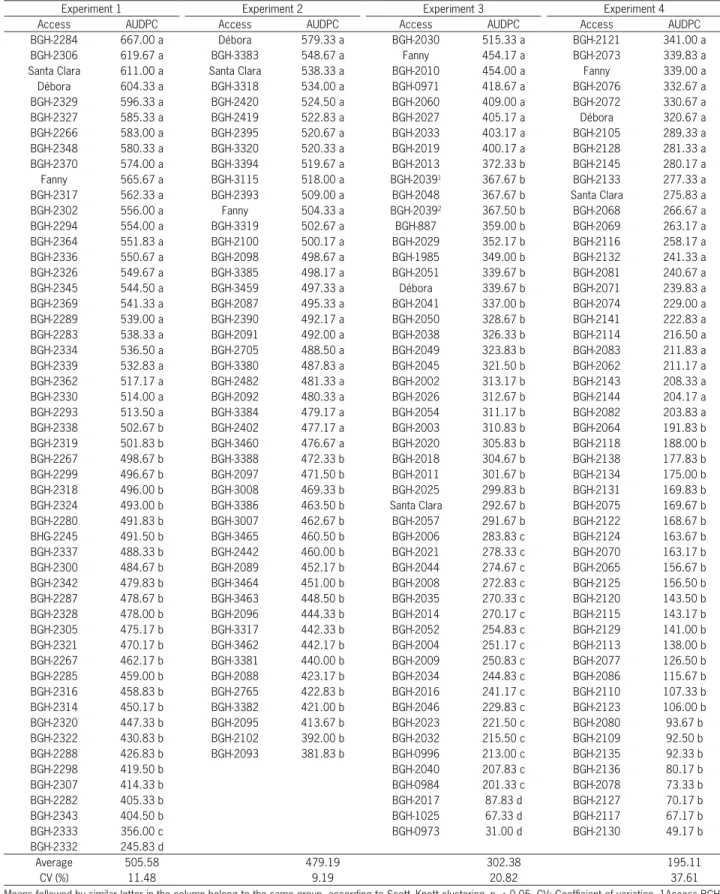
Table 1 − Area under the disease-progress curve (AUDPC) averages for one hundred and ninety tomato accessions, assessed for late-blight caused by Phytophythora infestans in four independent experiments.

Experiment 1 Experiment 2 Experiment 3 Experiment 4

Access AUDPC Access AUDPC Access AUDPC Access AUDPC

BGH-2284 667.00 a Débora 579.33 a BGH-2030 515.33 a BGH-2121 341.00 a

BGH-2306 619.67 a BGH-3383 548.67 a Fanny 454.17 a BGH-2073 339.83 a

Santa Clara 611.00 a Santa Clara 538.33 a BGH-2010 454.00 a Fanny 339.00 a

Débora 604.33 a BGH-3318 534.00 a BGH-0971 418.67 a BGH-2076 332.67 a

BGH-2329 596.33 a BGH-2420 524.50 a BGH-2060 409.00 a BGH-2072 330.67 a

BGH-2327 585.33 a BGH-2419 522.83 a BGH-2027 405.17 a Débora 320.67 a

BGH-2370 574.00 a BGH-3394 519.67 a BGH-2013 372.33 b BGH-2145 280.17 a

Fanny 565.67 a BGH-3115 518.00 a BGH-20391 _{367.67 b} _BGH-2133 _{277.33 a}

BGH-2317 562.33 a BGH-2393 509.00 a BGH-2048 367.67 b Santa Clara 275.83 a

BGH-2302 556.00 a Fanny 504.33 a BGH-20392 _{367.50 b} _BGH-2068 _{266.67 a}

BGH-2345 544.50 a BGH-3459 497.33 a Débora 339.67 b BGH-2071 239.83 a

BGH-2338 502.67 b BGH-2402 477.17 a BGH-2003 310.83 b BGH-2064 191.83 b

BGH-2319 501.83 b BGH-3460 476.67 a BGH-2020 305.83 b BGH-2118 188.00 b

BGH-2267 498.67 b BGH-3388 472.33 b BGH-2018 304.67 b BGH-2138 177.83 b

BGH-2324 493.00 b BGH-3386 463.50 b Santa Clara 292.67 b BGH-2075 169.67 b

BHG-2245 491.50 b BGH-3465 460.50 b BGH-2006 283.83 c BGH-2124 163.67 b

BGH-2337 488.33 b BGH-2442 460.00 b BGH-2021 278.33 c BGH-2070 163.17 b

BGH-2298 419.50 b BGH-2040 207.83 c BGH-2136 80.17 b

BGH-2307 414.33 b BGH-0984 201.33 c BGH-2078 73.33 b

BGH-2282 405.33 b BGH-2017 87.83 d BGH-2127 70.17 b

BGH-2343 404.50 b BGH-1025 67.33 d BGH-2117 67.17 b

BGH-2333 356.00 c BGH-0973 31.00 d BGH-2130 49.17 b

BGH-2332 245.83 d

Average 505.58 479.19 302.38 195.11

CV (%) 11.48 9.19 20.82 37.61

(4)

to create information able to measure ANN capacity to establish an optimum evaluation number for AUDPC prediction. In the third scenario, the replicates of 70 % of the genotypes were taken at the training stage and the genotypes remaining for validation processing, also con-sidering all evaluation combinations. This last scenario aimed to create information capable of establishing an optimum number of measurements and to evaluate net-work capability to extrapolate a learning curve for dif-ferent genotypes.

Analyses were performed using the GENES soft-ware (Cruz, 2013) and R Core team. ANN was performed with MATLAB®_{(Matrix Laboratory, version 7.10) using a}

script presented in the integration module of the GENES computer application (Cruz, 2013).

Data extrapolation

The implemented ANN with the best results in their respective experiments were considered for AUD-PC prediction in all experiments, i.e., for the

experi-ments for which they were trained and for those they were not trained. Only ANN that used two to three in-puts were considered.

Results and Discussion

Five evaluations were performed for phenotypic analysis in experiment 1, since, due to the fast progres-sion of disease, severity reached the plateau between the fourth and fifth evaluation. For the other experiments, six evaluations were performed. Accessions were sorted into groups using Scott-Knott clustering, according to the AUDPC. The groups with comparatively lower AUDPC values versus groups which had a susceptibility pattern were considered a possible source of resistance. There-fore, groups “c” and “d” of Experiment 1, group “b” of Ex-periment 2, groups “c” and “d” of ExEx-periment 3, and group “b” of Experiment 4 (Table 1) were considered potential sources of resistance to late blight because they showed lower severity than the susceptibility pattern groups.

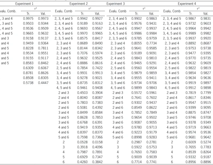
Table 2 − Average correlation for training and validation using different severity evaluation combinations. Training and validation were performed with four and five plants, respectively, using the same accession.

Evalu. Comb. r2 Evalu. Comb r2 Evalu. Comb r2 Evalu. Comb r2

Tr. Val. Tr. Val. Tr. Val. Tr. Val.

2, 3 and 4 0.9975 0.9973 2, 3, 4 and 5 0.9942 0.9927 2, 3, 4 and 5 0.9902 0.9863 2, 3, 4 and 5 0.9867 0.9831 2, 3 and 5 0.9503 0.9344 2, 3, 4 and 6 0.9189 0.9163 2, 3, 4 and 6 0.9576 0.9431 2, 3, 4 and 6 0.9732 0.9603 2, 4 and 5 0.9536 0.9509 2, 4, 5 and 6 0.9693 0.9567 2, 4, 5 and 6 0.9947 0.9937 2, 4, 5 and 6 0.9964 0.9942 3, 4 and 5 0.9665 0.9632 3, 4, 5 and 6 0.9970 0.9965 3, 4, 5 and 6 0.9986 0.9984 3, 4, 5 and 6 0.9989 0.9982 2 and 3 0.9158 0.9137 2, 3, 5 and 6 0.8575 0.8417 2, 3, 5 and 6 0.9785 0.9759 2, 3, 5 and 6 0.9937 0.9920 2 and 4 0.9459 0.9364 2, 3 and 4 0.8689 0.8490 2, 3 and 4 0.8055 0.7734 2, 3 and 4 0.8892 0.8687 2 and 5 0.8228 0.7811 2, 3 and 5 0.8144 0.8342 2, 3 and 5 0.9641 0.9585 2, 3 and 5 0.9753 0.9738 3 and 4 0.9534 0.9551 2, 3 and 6 0.7076 0.5974 2, 3 and 6 0.9189 0.9091 2, 3 and 6 0.9477 0.9395 3 and 5 0.9155 0.9117 2, 4 and 5 0.9632 0.9525 2, 4 and 5 0.9843 0.9810 2, 4 and 5 0.9770 0.9735 4 and 5 0.8583 0.8462 2, 4 and 6 0.8886 0.8616 2, 4 and 6 0.9465 0.9291 2, 4 and 6 0.9632 0.9609 2 0.6309 0.6067 2, 5 and 6 0.7854 0.7422 2, 5 and 6 0.9560 0.9554 2, 5 and 6 0.9822 0.9819 3 0.8781 0.8626 3, 4 and 5 0.9931 0.9913 3, 4 and 5 0.9879 0.9859 3, 4 and 5 0.9854 0.9827 4 0.8508 0.8305 3, 4 and 6 0.9278 0.9021 3, 4 and 6 0.9555 0.9411 3, 4 and 6 0.9634 0.9636 5 0.5738 0.4447 3, 5 and 6 0.8735 0.8312 3, 5 and 6 0.9734 0.9706 3, 5 and 6 0.9919 0.9897 4, 5 and 6 0.9461 0.9408 4, 5 and 6 0.9899 0.9843 4, 5 and 6 0.9912 0.9898 2 and 3 0.4503 0.3904 2 and 3 0.5572 0.5961 2 and 3 0.7819 0.7799 2 and 4 0.8040 0.8087 2 and 4 0.7641 0.7602 2 and 4 0.8617 0.8346 2 and 5 0.7803 0.7383 2 and 5 0.9302 0.9437 2 and 5 0.9547 0.9515 2 and 6 0.5081 0.4392 2 and 6 0.8549 0.8622 2 and 6 0.9399 0.9095 3 and 4 0.8499 0.8584 3 and 4 0.7852 0.7849 3 and 4 0.8875 0.8747 3 and 5 0.8628 0.7853 3 and 5 0.9654 0.9502 3 and 5 0.9746 0.9708 3 and 6 0.6768 0.6391 3 and 6 0.9087 0.9055 3 and 6 0.9378 0.9349 4 and 5 0.9419 0.9355 4 and 5 0.9780 0.9713 4 and 5 0.9719 0.9663 4 and 6 0.8397 0.8370 4 and 6 0.9223 0.9179 4 and 6 0.9574 0.9536 5 and 6 0.7598 0.7366 5 and 6 0.8998 0.9283 5 and 6 0.9681 0.9642

2 0.0528 0.0158 2 0.2987 0.2781 2 0.6009 0.5274

3 0.3918 0.4096 3 0.5922 0.5753 3 0.7655 0.7783

4 0.7987 0.7891 4 0.7650 0.7583 4 0.8539 0.8264

5 0.6929 0.7347 5 0.9009 0.9039 5 0.9332 0.9187

6 0.4260 0.3842 6 0.7714 0.7741 6 0.8956 0.8896

(5)

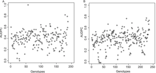
Using ANN to analyze the data in scenario 1 to evaluate tomato - P. Infestans pathosystem, resulted in expectations being met and were very efficient. ANN construction in this scenario provided a correlation coefficient (r2_{) similar to that observed in the training}

(Figure 1A) and validation (Figure 1B) stages, showing ANN capacity to predict the AUDPC, regardless of the model. Average quadratic error reached acceptable lev-els at both stages (9.4183.10−7_{and 3.067.10}−5_,

respec-tively). The best ANN had two neurons in the hidden layer, using the logistic sigmoid activation function. Sev-eral authors (Goyal, 2013) have reported the efficiency of neural networks in studies in terms of classification, prediction, and mainly in model adjustment, which was the case in the present study.

For scenario 2, which aimed at establishing a mini-mum optimini-mum number of evaluations (measurements) to predict the AUDPC, it was demonstrated that ANN are an efficient and appropriate tool for identifying with the lower number of evaluations during training and val-idation using the same set of genotypes. Results of the average correlation coefficient _{( )}_r2 _{between AUDPC}

val-ues and ANN predicted valval-ues during training and vali-dation stages are presented in Table 2. Using the fourth and fifth evaluation provided an _{( )}_r2 _{, during the}

net-work validation stage, greater than 84 % for Experiment 1, and greater than 93 % for the remaining experiments. In this case, three neurons were usually enough for the prediction process, regardless of the activation function. Considering the third, fourth and fifth evaluation, the

2

( )r exceeded 96 %, using four neurons in the hidden layer, where the logistic sigmoid activation function showed the best results. Results of this scenario imply the realization of a full evaluation in a reduced number of plants per genotype followed by a reduced number of evaluations in the plants to be predicted by ANN.

ANN were effective in predicting the AUDPC us-ing a lower number of evaluations to validate non trained genotypes in scenario 3, demonstrating their capacity to predict and extrapolate values. This implies using ANN to predict AUDPC without being necessarily trained for a given group of genotypes, since previous ANN training has been performed under the conditions of the current experiment, or that it does not have outstanding pecu-liarities when compared to the experiments for which ANN was trained. Considering only the fourth and fifth evaluation, the ANN was capable of predicting AUDPC with an _{( )}_r2 _{greater than 87 % in all experiments.}

AUD-PC values predicted by ANN showed an _{( )}_r2 _greater

than 93 % when using the third, fourth and fifth evalua-tions. Results are shown in Table 3. The ANN construct-ed showconstruct-ed architecture similar to the previous cases.

Grouping of the prediction averages performed by ANN were very similar, sometimes equal, to that formed through the conventional method (Table 4). Even though in both cases, AUDPC averages were very similar, some-times genotype classification had changed, but this change was not an obstacle to the selection of sources of resistance.

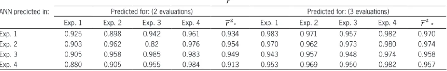
Potential ANN candidates were selected in sce-nario 3 where the extrapolation capacity was confirmed. The ANN were considered using two evaluations - the fourth and fifth – and then three evaluations – the third, fourth and fifth. Results were promising and are shown in Table 5. The _{( )}_r2 _{results between AUDPC and ANN}

predicted values, of an ANN trained to one experiment predicting the others considering two and three evalua-tions, exceeded 91 and 95 %, respectively.

Research concerning artificial intelligence has been showing remarkable advances since 1980’s, reflect-ing the practical use of ANN (Dreflect-ing et al., 2013). The capacity of learning from a set of examples and of

(6)

rately predicting desired responses has made possible an incremented ANN use in agricultural sciences as well as making valuable studies available for researchers in this field of study (Goyal, 2013). With respect to plant disease evaluations, the ANN have been used in image process-ing, as a means of evaluating disease severity, thus re-ducing the subjectivity of evaluation (Patil and Kumar, 2011; Tiger and Verma, 2013).

Considering that disease evaluation represents a significant investment in time, space, human and eco-nomic resources, the use of an efficient methodology to evaluate disease progress that saves resources is highly desirable. The AUDPC measurement of quantitative re-sistance evaluation for polycyclic pathogens, resulting from calculations from periodic evaluations, is extreme-ly common and necessary, such as in the present study. In this sense, ANN utilization represents an interesting alternative, since it has allowed for the selection of pu-tative sources of resistance with a reduced number of evaluations. Also, according to Mukherjee et al. (2010),

when evaluations are frequent during the outbreak they can inadvertently affect disease progress, given anthrop-ic interference.

This new paradigm could save land, fertilizers, water, supplies for training and management of tomato fields, besides the human resources that are necessary for maintenance of the experiments. The application of this approach is highly practical for the evaluation of ex-periments regardless of the model, still considering that factors like unbalancing are not a great problem. There-fore, ANN could improve the efficiency of the screening process of sources of resistance.

ANN also ensures the researcher, considering the tomato × late-blight pathosystem, uses all convention-al evconvention-aluations in only a few replicates of the experi-ment to train the ANN and later to estimate AUDPC for the other replicates of each genotype. This would imply a 0.97 correlation between estimated value, us-ing three evaluations as input, at nine, twelve and fif-teen dpi; and that would be obtained with six

evalua-Table 3 − Average correlations for training and validation using different combinations of severity evaluations. Training was used in 70 % of the accessions and validation in the other 30 % for each experiment.

Evalu. Comb. r2 Evalu. Comb r2 Evalu. Comb r2 Evalu. Comb r2

Tr. Val. Tr. Val. Tr. Val. Tr. Val.

2, 3 and 4 0.9948 0.9816 2, 3, 4 and 5 0.9955 0.9913 2, 3, 4 and 5 0.9910 0.9829 2, 3, 4 and 5 0.9872 0.9805 2, 3 and 5 0.9510 0.9408 2, 3, 4 and 6 0.9283 0.9014 2, 3, 4 and 6 0.9546 0.9319 2, 3, 4 and 6 0.9658 0.9741 2, 4 and 5 0.9529 0.9513 2, 4, 5 and 6 0.9728 0.9593 2, 4, 5 and 6 0.9954 0.9962 2, 4, 5 and 6 0.9967 0.9931 3, 4 and 5 0.9597 0.9745 3, 4, 5 and 6 0.9974 0.9961 3, 4, 5 and 6 0.9980 0.9988 3, 4, 5 and 6 0.9990 0.9982 2 and 3 0.9210 0.9020 2, 3, 5 and 6 0.9452 0.6202 2, 3, 5 and 6 0.9723 0.9911 2, 3, 5 and 6 0.9934 0.9925 2 and 4 0.9442 0.9397 2, 3 and 4 0.8720 0.8610 2, 3 and 4 0.7971 0.7435 2, 3 and 4 0.8824 0.8787 2 and 5 0.8160 0.7854 2, 3 and 5 0.9380 0.5986 2, 3 and 5 0.9589 0.9702 2, 3 and 5 0.9788 0.9666 3 and 4 0.9525 0.9626 2, 3 and 6 0.7160 0.5360 2, 3 and 6 0.9176 0.9034 2, 3 and 6 0.9572 0.9331 3 and 5 0.9084 0.9218 2, 4 and 5 0.9655 0.9519 2, 4 and 5 0.9848 0.9795 2, 4 and 5 0.9798 0.9715 4 and 5 0.8374 0.8744 2, 4 and 6 0.9138 0.8382 2, 4 and 6 0.9469 0.9126 2, 4 and 6 0.9707 0.9449 2 0.6091 0.6345 2, 5 and 6 0.8837 0.5545 2, 5 and 6 0.9484 0.9747 2, 5 and 6 0.9838 0.9788 3 0.8720 0.8674 3, 4 and 5 0.9926 0.9895 3, 4 and 5 0.9894 0.9827 3, 4 and 5 0.9863 0.9796 4 0.8224 0.8630 3, 4 and 6 0.9277 0.9027 3, 4 and 6 0.9539 0.9280 3, 4 and 6 0.9724 0.9492 5 0.4869 0.5369 3, 5 and 6 0.9273 0.5851 3, 5 and 6 0.9681 0.9879 3, 5 and 6 0.9902 0.9902 4, 5 and 6 0.9273 0.5851 4, 5 and 6 0.9871 0.9903 4, 5 and 6 0.9913 0.9874 2 and 3 0.4758 0.2661 2 and 3 0.5669 0.6290 2 and 3 0.7925 0.7597 2 and 4 0.8254 0.7958 2 and 4 0.7835 0.7143 2 and 4 0.8518 0.8412 2 and 5 0.8721 0.5105 2 and 5 0.9337 0.9548 2 and 5 0.9587 0.9421 2 and 6 0.5239 0.3738 2 and 6 0.8660 0.8405 2 and 6 0.9415 0.8968 3 and 4 0.8642 0.8710 3 and 4 0.7885 0.7510 3 and 4 0.8793 0.8815 3 and 5 0.9200 0.5466 3 and 5 0.9521 0.9699 3 and 5 0.9767 0.9635 3 and 6 0.6953 0.5426 3 and 6 0.9123 0.9000 3 and 6 0.9479 0.9260 4 and 5 0.9456 0.9351 4 and 5 0.9772 0.9741 4 and 5 0.9725 0.9694 4 and 6 0.8631 0.8084 4 and 6 0.9316 0.8892 4 and 6 0.9656 0.9332 5 and 6 0.8254 0.5126 5 and 6 0.8943 0.9706 5 and 6 0.9678 0.9610

2 0.0545 0.0116 2 0.2868 0.2600 2 0.6077 0.4844

3 0.4519 0.2538 3 0.5692 0.6348 3 0.7776 0.7696

4 0.8039 0.7827 4 0.7542 0.6878 4 0.8200 0.8491

5 0.8117 0.4555 5 0.8836 0.9515 5 0.9240 0.9193

6 0.4246 0.3514 6 0.7677 0.7928 6 0.8864 0.9059

(7)

Table 5 − Average correlations between predicted values by artificial neural networks (ANN) and conventional calculation according to Shaner and Finney (1977). The ANN used in each case predicted the area under the disease-progress curve of all plants from the other experiments.

ANN predicted in:

2

r

Predicted for: (2 evaluations) Predicted for: (3 evaluations)

Exp. 1 Exp. 2 Exp. 3 Exp. 4 2

r _* Exp. 1 Exp. 2 Exp. 3 Exp. 4 2

r _*

Exp. 1 0.925 0.898 0.942 0.961 0.934 0.983 0.971 0.957 0.982 0.970

Exp. 2 0.903 0.962 0.82 0.976 0.954 0.970 0.962 0.973 0.980 0.974

Exp. 3 0.905 0.958 0.985 0.983 0.949 0.943 0.957 0.948 0.974 0.958

Exp. 4 0.880 0.905 0.955 0.984 0.913 0.953 0.969 0.950 0.982 0.957

*Average correlation estimates considering only the experiments in which ANN was not trained.

Table 4 − Accession grouping according to Scott-Knott clustering, comparing area under the disease-progress curve (AUDPC) averages conventionally calculated, with six evaluations, and by artificial neural networks (ANN), with three evaluations (A) - 3rd_{, 4}th_{and 5}th_{- and two}

evaluations (B) - 4th_{and 5}th_. A

Access AUDPC ANN Access AUDPC ANN Access AUDPC ANN Access AUDPC ANN

BGH-2284 667.00 a 600.17 a BGH-3383 548.67 a 551.47 a BGH-971 418.67 a 417.76 a BGH-2105 289.33 a 296.55 a BGH-2266 583.00 b 582.29 a BGH-2393 509.00 b 507.52 b BGH-887 359.00 a 363.47 a BGH-2121 341.00 a 334.65 a BGH-2364 551.83 b 547.09 a BGH-2100 500.17 b 500.93 b Débora 339.67 b 333.28 b Débora 320.67 a 321.94 a BGH-2336 550.67 b 554.82 a BGH-3385 498.17 b 496.90 b BGH-2045 321.50 b 317.58 b Fanny 339.00 a 329.90 a BGH-2326 549.67 b 564.27 a BGH-2087 495.33 b 494.78 b BGH-2003 310.83 b 299.04 b BGH-2062 211.17 b 216.68 b BGH-2289 539.00 b 536.58 a BGH-2390 492.17 b 493.20 b BGH-2018 304.67 b 305.98 b BGH-2074 229.00 b 239.72 b BGH-2339 532.83 b 532.53 a BGH-2091 492.00 b 490.71 b BGH-2011 301.67 b 307.02 b BGH-2064 191.83 b 199.33 b BGH-2330 514.00 b 508.68 a BGH-2402 477.17 c 474.10 c BGH-2021 278.33 b 273.53 b BGH-2118 188.00 b 201.15 b BGH-2293 513.50 b 509.03 a BGH-3388 472.33 c 471.40 c BGH-2008 272.83 b 260.43 c BGH-2132 241.33 b 231.79 b BGH-2245 491.50 c 493.45 b BGH-2097 471.50 c 476.11 c BGH-2004 251.17 c 241.91 c BGH-2143 208.33 b 194.78 b BGH-2337 488.33 c 485.61 b BGH-3008 469.33 c 470.38 c BGH-2009 250.83 c 243.02 c BGH-2144 204.17 b 203.74 b BGH-2321 470.17 c 475.35 b BGH-2096 444.33 d 443.28 d BGH-2016 241.17 c 252.60 c BGH-2071 239.83 b 236.13 b BGH-2285 459.00 c 458.03 b BGH-3462 442.17 d 443.48 d BGH-2023 221.50 c 223.97 c BGH-2120 143.50 c 139.21 c BGH-2298 419.50 d 417.07 c BGH-2765 422.83 d 422.68 d BGH-2040 207.83 c 178.66 c BGH-2065 156.67 c 155.72 c

BGH-2282 405.33 d 405.06 c BGH-984 201.33 c 205.44 c BGH-2070 163.17 c 167.54 c

BGH-2343 404.50 d 406.38 c BGH-2017 87.83 d 95.06 d BGH-2117 67.17 d 66.37 d

B

Access AUDPC ANN Access AUDPC ANN Access AUDPC ANN Access AUDPC ANN

BGH-2306 619.67 a 585.70 a BGH-3318 534.00 a 536.61 a BGH-2010 454.00 a 485.30 a BGH-2145 280.17 a 268.77 a BGH-2266 583.00 a 575.78 a Fanny 504.33 a 504.41 a BGH-2033 403.17 a 407.11 b BGH-2116 258.17 a 246.87 a BGH-2294 554.00 a 571.32 a BGH-3319 502.67 a 508.86 a BGH-2019 400.17 a 399.35 b BGH-2071 239.83 a 222.34 a BGH-2336 550.67 a 548.26 a BGH-2100 500.17 a 495.55 a BGH-2048 367.67 a 376.75 b BGH-2114 216.50 a 236.31 a BGH-2339 532.83 b 535.09 a BGH-3385 498.17 a 494.42 a BGH-2039 367.67 a 385.52 b BGH-2083 211.83 a 210.67 a BGH2362 517.17 b 525.75 b BGH-2092 480.33 a 488.09a BGH-2039 367.50 a 363.48 b BGH-2062 211.17 a 215.40 a BGH-2283 538.33 b 520.05 b BGH-2097 471.50 b 480.76a BGH-887 359.00 a 365.38 b BGH-2082 203.83 a 191.84 a BGH-2330 514.00 b 502.60 b BGH-3386 463.50 b 467.65 b BGH-2041 337.00 a 342.44 b BGH-2064 191.83 a 188.55 a BGH-2245 491.50 b 491.53 b BGH-3007 462.67 b 468.02 b BGH-2003 310.83 a 294.80 c BGH-2122 168.67 a 149.04 b BGH-2300 484.67 b 489.36 b BGH-3476 460.50 b 462.54 b Santa Clara 292.67 b 287.34 c BGH-2124 163.67 a 146.66 b BGH-2276 498.67 b 488.88 b BGH-2089 452.17 b 453.04 b BGH-2006 283.83 b 274.49 c BGH-2115 143.17 b 134.85 b BGH-2321 470.17 c 476.19 b BGH-3317 442.33 b 452.07 b BGH-2021 278.33 b 267.60 c BGH-2086 115.67 b 113.03 b BGH-2322 430.83 c 443.79 c BGH-2765 422.83 c 425.98 c BGH-2052 254.83 b 244.59 c BGH-2135 92.33 b 80.43 b BGH-2288 426.83 c 427.93 c BGH-2093 381.83 c 383.91 d BGH-2046 229.83 b 242.47 c BGH-2136 80.17 b 82.28 b

BGH-2298 419.50 c 424.07 c BGH-0984 201.33 b 207.42 c BGH-2127 70.17 b 76.07 b

BGH-2333 356.00 c 346.93 d BGH-2017 87.83 c 103.90 d BGH-2130 49.17 b 40.51 b

tions, or by performing the evaluations only at 12 and 15 days, and have a 0.87 correlation. At first, the prac-tical use of this method could seem unviable regard-ing its practicability, since the researcher would have

(8)

ANN also proved to be efficient in AUDPC diction of non-trained genotypes. AUDPC values pre-dicted by the network are very close to those obtained using conventional calculation, and the classification of genotype groups also proved to be very similar or even identical in some cases (Table 4). Sometimes there was little change in the groups; however, it was observed that this was due to the insertion or exclusion of one or a few genotypes in a certain group, which alters the groups of the other genotypes. Nevertheless, this is not a problem to selecting sources of resistance, since the separation of genotypes with lower AUDPC continues to occur. Thus, the selection of sources of resistance us-ing AUDPC predicted by ANN is promisus-ing, since even with the changes in genotype groups, ANN was efficient in distinguishing genotypes which showed lower sever-ity averages. Apparently, the practical application of the strategy utilized in this scenario is difficult, because the researcher would have to evaluate 70 % of the plants during the measurement period (six measurements or evaluations), and only with the remaining is it possible to estimate AUDPC with a lower number of replicates. Notwithstanding, it is important to highlight the net-work capacity for extrapolating its learning for another group of accessions, and is, thus, effective in a broader approach.

ANN extrapolation that was generated from an experiment and test for the others proved to be very ef-fective in reflecting the conventional calculation (Table 5), making it the use of neural networks for this purpose unquestionable. This demonstrates the importance of maintaining databases which have, for example, mea-surements of disease severity, AUDPC, among others, so that in the near future it would be possible to implement an evaluation program using ANN, and take advantage

of all potentialities of this tool. We have demonstrated in this study that even when using a limited dataset, it was possible to estimate the AUDPC of experiments performed in different micro-sites and in different time frames. Thus, it was possible, for example, using severity data and the AUDPC of Experiment 1 (performed under atypical in Jan 2009), to infer about the AUDPC of acces-sions of Experiment 4 (installed after 10 months) with a correlation greater than 96 % using a reduced number of evaluations.

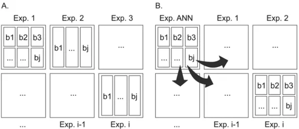
It is important to emphasize that the application of structured networks in the present study of AUDPC prediction in other experiments, should be recommend-ed with reservation, since database availability for ANN training is limited. Also, as previously reported, the prac-tical use of the strategies presented in scenario 1, 2 and 3, such as they were assessed, is also quite limited because it requires evaluations of samples from both plants and accessions to be applied. For this reason, the practical use of ANN in the routine work of a breeding program essentially necessitates a change in the current disease evaluation system paradigm (Figure 2A), even for tomato × P. infestans pathosystem. The new proposed paradigm (Figure 2B) presents a practical course of action which is based on planting representative accessions in a fraction of the experimental field (considering experimentation principles). These will serve as a basis for conventional evaluation and following ANN training along with his-torical data, are to be used in experiment prediction in the remaining experimental area, a contemporary of the ANN. In this, a reduced number of evaluations should be performed. Finally, we would like to emphasize that accumulating information in databases to be used in net-work training upgrading is necessary and should be rou-tine practice in breeding programs.

(9)

In this way, with the aim of screening the resistant accessions we recommend the application of this new paradigm and the performing of only two to three evalu-ations at 12 and 15 or at 9, 12 and 15 days after inocu-lation, respectively, followed by prediction using ANN. Moreover, ANN could be used for AUDPC predic-tion following the principles of other methods. Simko and Piepho (2012) proposed a series of evaluations for the AUDPC calculation, where different weights are at-tributed to the first and last evaluations, which are often penalized in other evaluation systems. ANN could, for example, be trained with the first, the last, and a reduced series of intermediate evaluations, and still allow for the AUDPC to be obtained, and reduce either costs or time.

Acknowledgements

To CAPES - Coordination for the Improvement of Higher Level Personnel, FAPEMIG - Minas Gerais State Foundation for Research Support and CNPq - Brazilian National Council for Scientific and Technological Devel-opment, for financial support and scholarships granted.

References

Abreu, F.B.; Silva, D.J.H.; Cruz, C.D.; Mizubuti, E.S.G. 2008. Inheritance of resistance to Phytophthora infestans

(Peronosporales, Pythiaceae) in a new source of resistance in tomato (Solanum sp. (formely Lycopersicon sp.) Solanales, Solanaceae). Genetics and Molecular Biology 31: 493-497. Braga, A.D.P.; Carvalho, A.P.L.F.; Ludermir, T.B. 2000. Artificial

Neural Networks: Theory and Applications = Redes Neurais Artificiais: Teoria e Aplicações. Livros Técnicos e Científicos, Rio de Janeiro, RJ, Brazil. (in Portuguese).

Corrêa, F.M.; Bueno Filho, J.S.S.; Carmo, M.G.F. 2009. Comparison of three diagrammatic keys for the quantification of late blight in tomato leaves. Plant Pathology 58: 1128-1133. Cruz, C.D. 2013. Genes: a software package for analysis

in experimental statistics and quantitative genetics. Acta Scientiarum Agronomy 35: 271-276.

Ding, S.; Li, H.; Su, C.; Yu, J.; Jin, F. 2013. Evolutionary artificial neural networks: a review. Artificial Intelligence Review 39: 251-260.

Ehret, A.; Hochstuhl, D.; Gianola, D.; Thaller, G. 2015. Application of neural networks with back-propagation to genome-enabled prediction of complex traits in Holstein-Friesian and German Fleckvieh cattle. Genetics Selection Evolution 47: 22.

Ferrandino, F.J.; Elmer, W.H. 1992. Reduction in tomato yield due to Septoria leaf spot. Plant Disease 76: 208-211.

Gianola, D.; Okut, H.; Weigel, K.A.; Rosa, G.J. 2011. Predicting complex quantitative traits with Bayesian neural networks: a case study with Jersey cows and wheat. BMC Genetics 12: 87. Goyal, S. 2013. Artificial neural networks in vegetables: a

comprehensive review. Scientific Journal of Crop Science 2: 75-94.

Irzhansky, I.; Cohen, Y. 2006. Inheritance of resistance against

Phytophthora infestans in Lycopersicon pimpinellifolium L3707. Euphytica 149: 309-316.

Jeger, M.; Viljanen-Rollinson, S. 2001. The use of the area under the disease-progress curve (AUDPC) to assess quantitative disease resistance in crop cultivars. Theoretical and Applied Genetics 102: 32-40.

Mukherjee, A.K.; Mohapatra, N.K.; Nayak, P. 2010. Estimation of area under the disease progress curves in a rice-blast pathosystem from two data points. European Journal of Plant Pathology 127: 33-39.

Nowicki, M.; Foolad, M.R.; Nowakowska, M.; Kozik, E.U. 2012. Potato and tomato late blight caused by Phytophthora infestans: an overview of pathology and resistance breeding. Plant Disease 96: 4-17.

Peixoto, L.A.; Bhering, L.L.; Cruz, C.D. 2015. Artificial neural networks reveal efficiency in genetic value prediction. Genetics and Molecular Research 14: 6796-6807.

Patil, J.K.; Kumar, R. 2011. Advances in image processing for detection of plant diseases. Journal of Advanced Bioinformatics Applications and Research 2: 135-141.

Shaner, G.; Finney, R. 1977. The effect of nitrogen fertilization on the expression of slow-mildewing resistance in Knox wheat. Phytopathology 67: 1051-1056.

Silva, G.N.; Tomaz, R.S.; Castro, I.S.; Nascimento, M.; Bhering, L.L. 2014. Neural networks for predicting breeding values and genetic gains. Scientia Agricola 71: 494-498.

Simko, I.; Piepho, H.P. 2012. The area under the disease progress stairs: calculation, advantage, and application. Phytopathology 102: 381-389.