Load cell adoption in an electronic drag force flowmeter
Antonio Pires de Camargo
1; Tarlei Arriel Botrel
1*; Ricardo Godoi Vieira
2; Marinaldo
Ferreira Pinto
1; Lucas Melo Vellame
11
USP/ESALQ – Depto. de Engenharia de Biossistemas, C.P. 09 – 13418-900 – Piracicaba, SP – Brasil.
2
ITA/IEC – Área de Informática, Pça. Marechal Eduardo Gomes, 50 – 12228-900 – São José dos Campos, SP – Brasil.
*Corresponding author <[email protected]>
ABSTRACT: This research introduces the development of an electronic flowmeter based on the drag force that a body experiences when immersed in a fluid stream. Its main goal was the development of an Electronic Drag Force Flowmeter (EDFF) using a load cell, as well as the evaluation of its performance parameters. The developed flowmeter should not require specialized labor, equipments, computers or any sophisticated and complex method, providing an easy and accurate way of flow estimation. This research was carried out in the following stages: (i) EDFF mechanical structure development; (ii) data acquisition system and embedded software design; and (iii) evaluation of EDFF performance parameters. EDFF has routines for instantaneous flow rate measurement, interactive calibration, and also several flow meter parameter adjustments, allowing data transmission via a RS-232 protocol. The real-time flow measurement task updates values of instantaneous flow rate each seven seconds, enabling unit selection. The interactive calibration routine guides users during all calibration process showing instructions on EDFF’s display. A data digital filtering procedure was implemented in an embedded software using the Grubbs’ Test in order to identify and to remove outliers from the acquired data. The Method of Least Squares was also implemented in the embedded software in order to calculate the fitting model coefficients on the calibration procedure. This flowmeter is able to work from 1.94 to 7.78 dm3 s–1 with an uncertainty of ± 5.7%. The coefficient of local head loss (K) was close to 0.55 for Reynolds number values higher than 105. The developed EDFF is a low-cost and stand-alone system with potential for agricultural applications.
Key words: technology innovation, flow measurement, electronics on agriculture
Medidor de vazão eletrônico com célula de carga
RESUMO: Este estudo apresenta o desenvolvimento de um medidor de vazão baseado na força de arraste que atua em um corpo imerso em uma corrente líquida. O principal objetivo foi o desenvolvimento de um Medidor de Vazão Eletrônico tipo Força (MVEF) utilizando célula de carga, bem como a avaliação do desempenho do equipamento. Esta pesquisa foi executada nas seguintes etapas: (i) desenvolvimento da estrutura mecânica do MVEF; (ii) desenvolvimento do sistema de aquisição de dados e do software embarcado; e (iii) avaliação dos parâmetros de desempenho do MVEF. O medidor de vazão desenvolvido possibilita a transmissão de dados via serial (RS-232) e possui rotinas para medição de vazão instantânea, calibração interativa e opções para ajuste de alguns parâmetros de funcionamento. O Teste de Grubbs foi utilizado no software embarcado com a finalidade de identificar e remover dados inconsistentes do conjunto amostral, sendo, portanto, um procedimento de filtragem digital de dados. A rotina de calibração do medidor de vazão consta de um algoritmo que utiliza o Método dos Mínimos Quadrados para determinação dos coeficientes de ajuste do modelo adotado. O medidor de vazão desenvolvido opera na faixa de 1,94 a 7,78 dm3 s–1 com incerteza de ± 5,7%. O coeficiente de perda de carga localizada característico do medidor de vazão foi de aproximadamente 0,55 para condições com Número de Reynolds superior a 105. O medidor de vazão desenvolvido apresenta baixo custo, sendo viável para utilização em aplicações agrícolas.
Palavras-chave: inovação tecnológica, hidrometria, eletrônica na agricultura Introduction
The initial spurs to flow measurement were agricul-tural requirements and necessity to evaluate water con-sumptions by the users in Egyptian, Roman and Chinese civilizations (Upp and La Nasa, 2002). From the 20th century onwards several new concepts of flowmeters were developed using electronic devices. The impact of new materials, processes, electronics and microproces-sors allows a widespread commercial development of modern flowmeter technology (Cascetta, 1995).
experi-ences when immersed in a fluid stream are hardly found or ment ioned in literature (Merzkirch, 2005). This kind of flowmeters can be used in a wide variety of applications as follows: general liquid or gas application, hot liquids, steam, slurries and particle flows, liquid and gas mixtures (Furness, 1991). In addition, target flowmeters appear to be suitable for use in food industry dealing with fluid products since these meters are easy to be cleaned and sanitized (Greene, 1993).
This research had as main objective the development of an Electronic Drag Force Flowmeter (EDFF) as well as the evealuation of its performance parameters. The developed flowmeter should not require specialized labor, equipment, computers or any sophisticated and complex method, pro-viding an easy and accurate way of measuring flow. More-over, the EDFF emerged according to innovative ideas be-coming a new and low-cost option available to flow mea-surement in closed conduits.
Material and Methods
Drag forces (Fd) act on bodies immersed in incompress-ible fluid streams and they can be calculated by eq. (1) de-pending on a drag coefficient (CD), characteristic area of the body (A), density of fluid (ρ), and flow velocity (u).
2 ²
ρ
=
D D
F C u A (1)
The frontal or projected area A that intercepts perpen-dicularly the flow is a constant. The density of fluid is a function of both the pressure and the temperature. The wa-ter density depends on its temperature and can also be con-sidered as a constant since the temperature does not change during a measurement process. For turbulent conditions, the flow velocity in closed conduits varies according to ra-dius (r). The average flow velocity (V) is generally detected at a distance between 0.7 and 0.8 r from the center posi-tion of a closed conduit (Neves, 1974). Aspects related to swirls and velocity profiles with distorted shapes are not taken into account once it is not the main purpose of this research. In an incompressible flow and in situations in which the body is completely immersed in the fluid, the drag coefficient (CD) depends mainly on the Reynolds num-ber (Re) and shape of the body. For these situations Re is determined by eq. (2), based on flow velocity (u), kinematic viscosity (v), and the characteristic dimension of the body (l) (Munson et al., 2004).
Re=u l
v (2)
In this research the force caused by the fluid flow acts on a target disc whose surface is oriented perpendicular to the flow direction. The target was attached to the inferior extrem-ity of a cylindrical metal beam. The drag causes a lower pres-sure area at the rear surface of the target, producing a net force that is transferred to the beam. A load cell was attached to upper extremity of the beam. Strain gauges measure the
deflection of the load cell due to drag force acting on target and on the immersed part of the cylindrical beam (Figure 1). The force acting on the target is measured directly instead of measuring the differential pressure, which produces a force on the target, proportional to the square of the flow rate. It was also mentioned by Baker (2000), that target flowmeters for Re values higher than 4000 have a drag force proportional to the square of the velocity. Therefore, ana-lyzing in the simplest way, the flow rate (Q) measured by target flowmeters may be estimated by eq. (3), in which k is assumed as a constant coefficient. A similar equation was mentioned by Delmée (2003) using the differential pressure instead of the drag force.
= D
Q k F (3)
The EDFF design, manufacturing, and evaluation were accomplished in the following stages: EDFF mechanical struc-ture development; hardware and embedded software design; and evaluation of EDFF performance parameters.
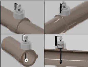
The EDFF mechanical structure was completely de-signed using Computer Aided Design (CAD) environment tool in order to reduce mechanical faults. With this tool was possible to reduce time and waste of resources. Figure 2 presents the functional model developed by the CAD tool.
Figure 1 – Fundamental structure of the Electronic Drag Force Flowmeter and the velocity profile schematic for turbulent flow conditions.
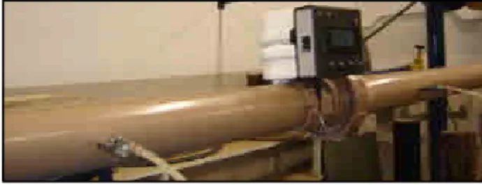
A target disc of 20 mm diameter and 1 mm thickness was attached to a steel cylindrical beam of 118 mm length and 7 mm diameter. These objects were assembled inside a 66 mm diameter pipeline. The center of the target disc was positioned 0.7 r from the center of the pipe transversal sec-tion in order to ensure the average velocity acting on the target. A 46.1 mm-long portion of the beam was also im-mersed. The beam was drilled 72 mm above the center of target to insert a metal stick of 2 mm thickness. It pro-vided a rotation axis for the transference of the force from target to a load cell. A bending beam load cell was used with 4.9 N capacity, sensitivity of 0.002 v v–1 and accuracy of ± 0.1%. The sealing mechanism comprises rubber seal rings, metal washers and some PVC fittings. Other PVC and metal fittings were manufactured and used to develop the EDFF mechanical structure (Figure 1 and 2). Figure 3 shows the EDFF developed in this research installed on a pipeline.
An electromagnetic flowmeter (uncertainty of ± 0.5%) was used as the reference meter in calibration procedures. The EDFF and the electromagnetic flowmeter were in-stalled in a pipeline of 66 mm diameter. A gate valve was also installed 1 m downstream of the electromagnetic flow-meter in order to control the flow rate. Figure 4 presents a schematic diagram of experimental setup. The evaluation tests were performed under a constant pressure condition of 98.1 kPa. The water temperature during tests remained close to 293 K.
The flowmeter Data Acquisition System (DAS) was de-veloped in order to acquire and process the output signal from the load cell converting it into flow rate. The DAS provides routines for instantaneous flow rate measurement, interactive calibration, and also several flowmeter measur-ing parameters adjustment. Durmeasur-ing all development there was a great concern regarding the routine creation in order
to ensure an easy way to work with the EDFF. The hard-ware of the DAS is comprised by the following devices: instrumentation amplifier, microcontroller, serial converter device, liquid-crystal display (LCD), capacitors, resistors, volt-age regulators, control buttons, and power supply of 15 Vcc.
After assemblage of these items, the DAS hardware is able to: (i) provide a precision voltage reference of 10 Vcc for load cell supply; (ii) amplify the load cell out-put signals; (iii) convert the amplified outout-put signals into digital data using the internal A/D converter of the microcontroller with 10 bits of resolution; (iv) per-f orm d ig ital d a t a proc es s ing us ing a P I C1 8 F4 5 5 0 microcontroller; (v) display instructions and informa-tion on a LCD; (vi) access routines using control but-tons; and (vii) allow sending the acquired data to a mi-crocomputer.
The embedded software in the DAS provides the fol-lowing tasks: (i) access a real-time flow measurement that up-dates values of instantaneous flow rate each seven seconds, enabling unit selection (m3
s–1 , m3
h–1 , L s–1
, and L h–1 ); (ii) access an interactive calibration guiding user along all cali-bration process; (iii) perform several flowmeter parameter adjustments; and (iv) allow the acquired data transmission via RS-232 protocol to a microcomputer (Figure 5).
A data digital filtering procedure was implemented in the embedded software using the Grubbs’ Test, in order to iden-tify outliers and remove them from the acquired data (ISO 5168, 1985). This procedure was used for instantaneous flow rate measurement and for interactive calibration routines. In this research, data is designated as “raw data” before digital filtering, while data is designated as “processed data” after digital filtering.
The interactive calibration task guides the user along the calibration procedure. The flowmeter LCD displays sequen-tial instructions to the user. Along this procedure the flow rate data is gathered from 0.00 to 8.33 dm3 s–1. The acquired data necessary to calculate the fitting model coefficients is stored in a microcontroller (RAM memory). The obtained coefficients for each calibration task are stored in the microcontroller memory allowing changes when necessary (EEPROM memory).
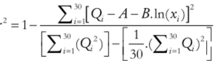
The Method of Least Squares was implemented in the embedded software in order to calculate the fitting model coefficients. A logarithmic model was used to predict the flow rate (eq. 4), and regression coefficients (A and B) were deter-mined by eq. 5. The determination coefficient (r2
) was calcu-lated by eq. 6 (Souza, 2009).
Q = A + B ln (x) (4)
[
]
[
]
30 30
1 1
30 30 30
2
1 1 1
30 ln( )
ln( ) ln( ) ln( )
= =
= = =
⎧ +⎡ ⎤ =
⎪ ⎢ ⎥
⎪ ⎣ ⎦
⎨
⎡ ⎤ ⎧ ⎫
⎪ +⎨ ⎬ =
⎢ ⎥
⎪⎣ ⎦ ⎩ ⎭
⎩
∑
∑
∑
∑
∑
i i
i i
i i i i
i i i
A x B Q
x A x B Q x (5)
Figure 4 – Schematic diagram of experimental setup. EDFF = Electronic Drag Force Flowmeter.
[
]
30 2
2 1
30 2 30 2
1 1
.ln( ) 1
1
( ) .( )
30
i i
i
i i
i i
Q A B x
r
Q Q
=
= =
− − = −
⎡ ⎤
⎡ ⎤ − ⎢ ⎥
⎣ ⎦ ⎣ ⎦
∑
∑
∑
(6)where: A and B are Regression coefficients; xi: ith processed data; Qi: ith
value of reference flow rate.
Taking into account the DAS features it is reasonable to consider EDFF as a stand-alone system. All the math-ematical processes are performed by the microcontroller. The system allow s data trans mission from the microcontroller to an external microcomputer via a serial port (RS-232). The data transmission to a microcomputer may be useful to create reports, charts, and also allows per-forming other complex routines. One of the DAS chal-lenges was to define the sample size (n). Three replicates of two sample sizes were evaluated (n = 30 and n = 500). These tests were performed on three different flow condi-tions (0.0, 4.17, and 6.25 dm3
s–1
). A sampling interval of 250 milliseconds was used.
Statistical and performance parameters like repeatabil-ity, hysteresis, conformrepeatabil-ity, and uncertainty interval limits, as well as curve model fitting were determined based on four tests. Data was gathered by increasing and decreas-ing flow rates, changdecreas-ing values on intervals of 0.28 dm3 s–1 in a range from 0.0 to 8.33 dm3 s–1. The flow rate was controlled using a gate valve and observing flow rates in an electromagnetic flowmeter installed in series down-stream from EDFF (Figure 4). The determination of the EDFF uncertainty limit (U) was performed adopting pro-cedures presented by ISO 5168 (1985). The equation used to combine bias errors (B) and random errors (S) is pre-sented below:
2 2
(2 )
= +
U B S (7)
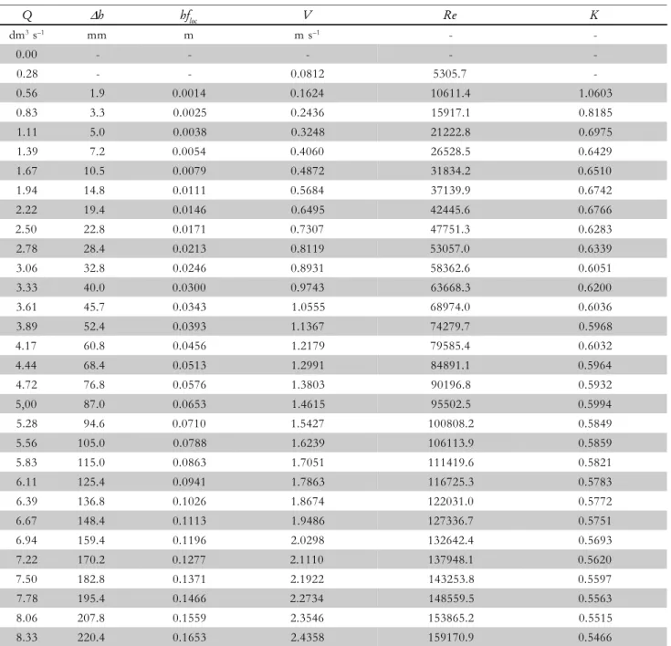
Local head losses are originated due to sudden changes in flow condition caused by pipe fittings or other flow in-terferences increasing flow turbulence and energy loss (Porto, 1998). The local head loss coefficient (K) of the EDFF was determined experimentally. The head loss was calculated based on eqs 8 and 9. A differential manometer was installed dis-tanced of 0.4 m upstream and downstream from the EDFF. A manometric fluid of density (d) 1750 kg m–3 (Figure 6) was used.
2
2
=
loc V
hf K
g (8)
0.75
= Δ
loc
hf h (9)
where: hfloc: local head loss (m); K coefficient of local head loss ( - ); V average flow velocity (m s–1
); g: acceleration of gravity = 9.81 m s–2
; Δh: differential pressure between 1 and 2 (m).
Results and Discussion
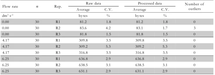
Sample size determination is an important and hard stage on planning any gathering data or sampling process (Dattalo, 2008). As larger the sample size is, the smaller the expected random error will be (Cacuci, 2003; Drosg, 2007). Any con-troller has limited storage and processing capacity due to price and physical space. Large sample sizes require more process-ing time to update and display data for users. Hence, sample size is a constraint aspect for an electronic flowmeter devel-opment. Grubbs’ Test is a recommended mathematical pro-cedure for data processing in flow measurement systems (ISO 5168, 1985). Applying this procedure to a set of data with 500 values (n = 500), considering three different flow rates (0.00, 4.17, and 6.25 dm3 s–1), and three replicates we obtained the results shown in Table 1.
Figure 6 – Differential manometer and pressure taps arrangement.
Flow rate n Rep. Raw data Processed data N umber of
outliers
Average C .V. Average C .V.
dm3 s–1 by tes % by tes %
0.00 500 R1 82.6 3.0 82.5 1.8 15
0.00 500 R2 82.7 3.4 82.4 1.8 17
0.00 500 R3 81.8 4.4 81.8 1.5 18
4.17 500 R1 312.0 4.2 312.0 4.2 0
4.17 500 R2 313.4 4.3 313.4 4.3 0
4.17 500 R3 317.9 7.2 319.0 4.4 2
6.25 500 R1 636.9 2.7 636.9 2.7 0
6.25 500 R2 633.7 5.6 635.7 2.7 2
6.25 500 R3 633.2 2.6 633.2 2.6 0
Table 1 – Summarized results obtained to sample size of 500 values (n = 500).
Flow rate n Rep. Raw data Processed data N umber of
outliers
Average C .V. Average C .V.
dm3 s–1 by tes % by tes %
0.00 30 R1 81.2 1.8 81.2 1.8 0
0.00 30 R2 83.6 4.2 83.1 1.7 3
0.00 30 R3 81.8 1.5 81.8 1.5 0
4.17 30 R1 309.8 3.5 309.8 3.5 0
4.17 30 R2 309.2 5.3 309.2 5.3 0
4.17 30 R3 316.8 3.5 316.8 3.5 0
6.25 30 R1 636.8 2.9 636.8 2.9 0
6.25 30 R2 638.5 3.1 638.5 3.1 0
6.25 30 R3 631.1 2.9 631.1 2.9 0
Table 2 – Summarized results obtained to sample size of 30 values (n = 30).
During tests with flow rate of 0.00 dm3 s–1, we detected and eliminated 15 outliers from replicate 1 (R1), 17 outli-ers from replicate 2 (R2) and 18 outlioutli-ers from replicate 3 (R3). The resulted average of the final data under this flow condition was 82.2 bytes. By setting flow rate to 4.17 dm3 s–1
we found 2 outliers in R3 resulting an average of
pro-cessed data of 314.8 bytes. Propro-cessed data for the 6.25 dm3 s–1
flow condition we found two outliers in R2, resulting an average of 635.3 bytes. The same tests were performed with sample size 30 (n = 30) applying the Grubb’s Test procedure, as shown in Table 2. We found three outliers in R2 for the 0.00 dm3
s–1
flow condition. The small number of detected outliners was expected once measurement sys-tems generally acquire a little number of data and the prob-ability of outlier occurrence is small (Rabinovich, 2005). Dif-ferences in the processed data were very small between sample sizes of 500 and 30 (Tables 1 and 2). Therefore, it is reasonable to consider that it is not necessary to process more than 30 values in each sampling cycle. Using n = 30 the required time to gather, process, and update data was close to seven seconds.
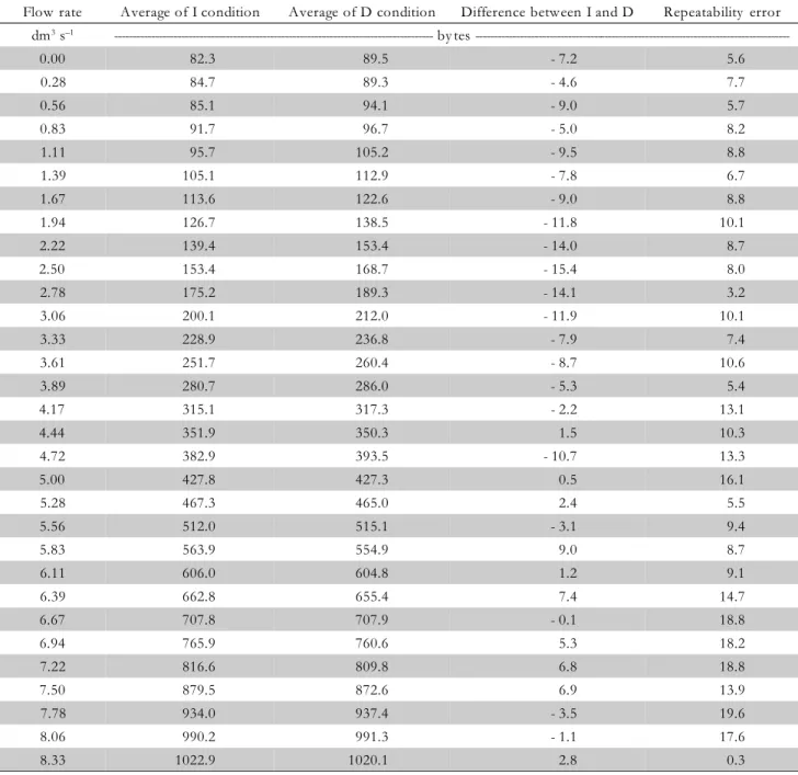
reso-lution was used, the value of FS is reached for 1024 bytes. To estimate the hysteresis error tests of increasing and de-creasing flow rate values were carried out (Table 4). The larg-est difference obtained between increasing and decreasing flow rates was 15.4 bytes respectively to 2.50 dm3 s–1
. There-fore, the hysteresis error was estimated to be ± 1.5% based on FS.
As mentioned for eq. (3), Q measured by target flowmeters may be estimated as a function of FD and the constant k. The load cell installed in the developed EDFF has a linear output signal. The force that acts on load cell (FLC) is not exactly equal to the drag force since there is a distance above the fulcrum (rotation axis) of 46 mm (L1)
and below the fulcrum of 72 mm (L2). Then, FD can also be expressed by eq. (10), where x is processed data, k1 and k2 are constant values determined by load cell characteris-tic:
1
1 2
2
( )
= +
D
L
F k x k
L (1 0)
Analyzing eq. (3) and eq. (10):
1
1 2
2
( )
= + L
Q k k x k
L (1 1)
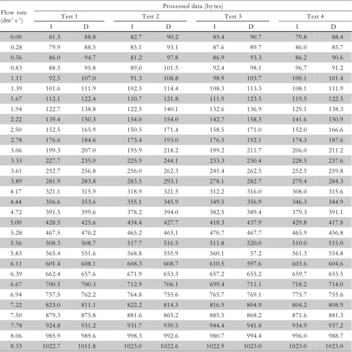
Table 3 – Data gathered in order to estimate the Electronic Drag Force Flowmeter performance parameters.
I - Processed data from increasing flow condition; D - Processed data from decreasing flow condition. Flow rate
(dm3 s–1)
Processed data (by tes)
Test 1 Test 2 Test 3 Test 4
I D I D I D I D
0.00 81.3 88.8 82.7 90.2 85.4 90.7 79.8 88.4
0.28 79.9 88.5 85.1 93.1 87.6 89.7 86.0 85.7
0.56 86.0 94.7 81.2 97.8 86.9 93.3 86.2 90.6
0.83 88.5 95.8 89.0 101.5 92.4 98.1 96.7 91.2
1.11 92.5 107.0 91.3 108.8 98.9 103.7 100.1 101.4
1.39 101.6 111.9 102.5 114.4 108.3 113.3 108.1 111.9
1.67 112.1 122.4 110.7 121.8 111.9 123.5 119.5 122.5
1.94 122.7 138.8 122.5 140.1 132.6 136.9 129.1 138.3
2.22 139.4 150.3 134.0 154.0 142.7 158.3 141.6 150.9
2.50 152.5 165.9 150.5 171.4 158.5 171.0 152.0 166.6
2.78 176.6 184.6 173.4 193.0 176.5 192.1 174.3 187.6
3.06 199.3 207.0 195.9 218.2 199.2 211.7 206.0 211.2
3.33 227.7 235.0 225.9 244.1 233.3 230.4 228.5 237.6
3.61 252.7 256.8 256.0 262.3 245.4 262.5 252.5 259.8
3.89 281.9 283.8 283.5 293.1 278.1 282.7 279.4 284.3
4.17 321.1 315.9 318.9 321.5 312.2 316.0 308.0 315.6
4.44 356.6 353.6 355.1 345.9 349.5 356.9 346.3 344.9
4.72 391.5 399.6 378.2 394.0 382.5 389.4 379.3 391.1
5.00 428.5 425.6 434.4 427.7 418.3 437.9 429.8 417.8
5.28 467.5 470.2 465.2 465.1 470.7 467.7 465.9 456.8
5.56 508.3 508.7 517.7 516.5 511.8 520.0 510.0 515.0
5.83 565.4 551.6 568.8 555.9 560.1 57.2 561.3 554.8
6.11 601.4 608.1 608.3 608.7 610.5 597.6 603.6 604.6
6.39 662.4 657.6 671.9 653.3 657.2 655.2 659.7 655.5
6.67 700.5 700.3 712.9 706.1 699.4 711.1 718.2 714.0
6.94 757.5 762.2 764.8 755.6 765.7 769.1 775.7 755.6
7.22 823.0 811.1 822.2 814.3 816.9 804.9 804.2 808.9
7.50 879.3 875.8 881.6 865.2 885.5 868.2 871.6 881.3
7.78 924.8 931.2 931.7 939.5 944.4 941.8 934.9 937.2
8.06 985.9 989.6 998.3 992.6 980.7 994.4 996.0 988.7
Flow rate Average of I condition Average of D condition Difference between I and D Repeatability error dm3 s–1 - by tes
---0.00 82.3 89.5 - 7.2 5.6
0.28 84.7 89.3 - 4.6 7.7
0.56 85.1 94.1 - 9.0 5.7
0.83 91.7 96.7 - 5.0 8.2
1.11 95.7 105.2 - 9.5 8.8
1.39 105.1 112.9 - 7.8 6.7
1.67 113.6 122.6 - 9.0 8.8
1.94 126.7 138.5 - 11.8 10.1
2.22 139.4 153.4 - 14.0 8.7
2.50 153.4 168.7 - 15.4 8.0
2.78 175.2 189.3 - 14.1 3.2
3.06 200.1 212.0 - 11.9 10.1
3.33 228.9 236.8 - 7.9 7.4
3.61 251.7 260.4 - 8.7 10.6
3.89 280.7 286.0 - 5.3 5.4
4.17 315.1 317.3 - 2.2 13.1
4.44 351.9 350.3 1.5 10.3
4.72 382.9 393.5 - 10.7 13.3
5.00 427.8 427.3 0.5 16.1
5.28 467.3 465.0 2.4 5.5
5.56 512.0 515.1 - 3.1 9.4
5.83 563.9 554.9 9.0 8.7
6.11 606.0 604.8 1.2 9.1
6.39 662.8 655.4 7.4 14.7
6.67 707.8 707.9 - 0.1 18.8
6.94 765.9 760.6 5.3 18.2
7.22 816.6 809.8 6.8 18.8
7.50 879.5 872.6 6.9 13.9
7.78 934.0 937.4 - 3.5 19.6
8.06 990.2 991.3 - 1.1 17.6
8.33 1022.9 1020.1 2.8 0.3
Table 4 – Values used on analysis of repeatability and hysteresis errors.
I - Processed data from increasing flow condition; D - Processed data from decreasing flow condition.
By grouping some of the constant values, a theoretical model to estimate Q is given by:
3 4
( )
= +
Q k k x k (1 2)
The fitting model used to convert processed data (bytes) into flow rate values (dm3
s–1
) was determined from average values presented in Table 3. The theoretical model (eq. 12) was compared with a logarithmic model presented as eq. (4). The choice of the adopted model was based on the coeffi-cient of determination (r2) (Figure 7).
Theoretical model:
0.3633 0.5405 42.9194
= −
Q x (1 3)
r2 = 0.938
Logarithmic model:
Q = 2.992ln (x) –12.89 (14)
r2 = 0.993
Based on r2
pro-cess of the EDFF mechanical structure, which was hand-made and it probably was harmflul for the EDFF perfor-mance.
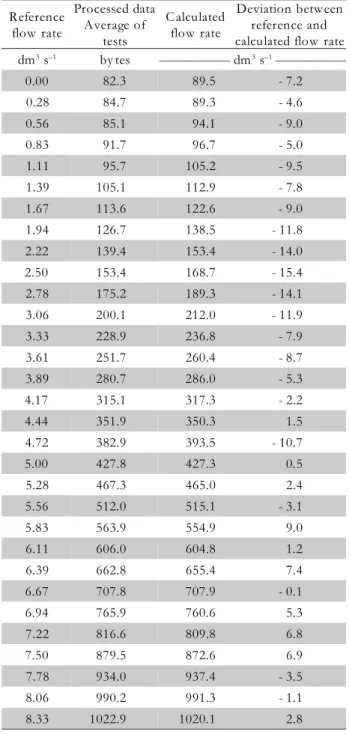
When a mathematic model that describes data distri-bution is non linear, the term conformity is used instead of linearity (Delmée, 2003). Based on the logarithmic model the conformity analysis resulted in a maximum deviation of ± 0.50 dm3 s–1 for a reference flow rate of 8.33 dm3 s–1. Hence, the conformity error of range from 0.00 to 8.33 dm3 s–1 is ± 6.0%. If the measurement range would be restricted to flow rates between 0.28 and 8.06 dm3 s–1 the maximum conformity error would be 0.31 dm3
s–1
(± 3.7 %). In the same way, if the range would be even more limited, from 1.94 to 7.78 dm3 s–1 the respective conformity error would be ± 0.22 dm3 s–1 (± 2.7%) (Table 5).
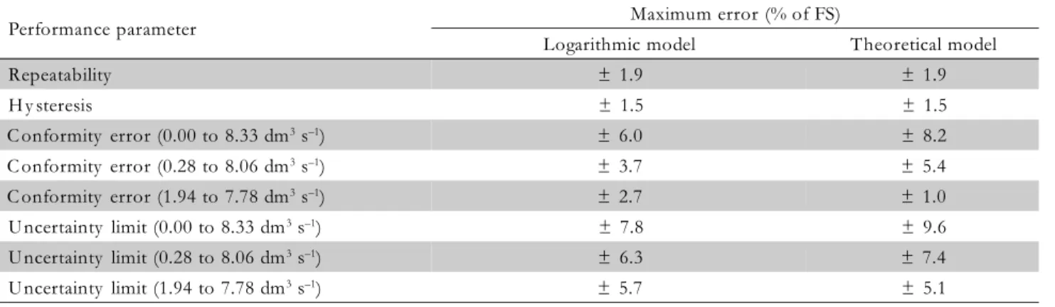
According to the procedure of ISO 5168 (1985) the estimated random error limits are equal to ± 0.21 dm3 s–1. This result was obtained combining random errors of repeatability (± 1.9% or ± 0.16 dm3 s–1) and hyster-esis (± 1.5% or ± 0.13 dm3
s–1
), on the range 0.00 to 8.33 dm3
s–1
. The bias error limits were estimated for three flow measurement ranges. The conformity error was the only evaluated type of bias error. Based on ranges from 0.00 to 8.33 dm3
s–1
, from 0.28 to 8.06 dm3 s–1
, and from 1.94 to 7.78 dm3 s–1, the respective bias errors were ± 6% (± 0.5 dm3 s–1), ± 3.7% (± 0.31 dm3 s–1), and ± 2.7% (± 0.22 dm3 s–1). By merging bias error lim-its with random error limlim-its for the three flow measure-ment ranges, the uncertainty error limits were ± 7.8%, ± 6.3%, and ± 5.7%, respectively.
Otherwise, if the theoretical model would used to ex-press flow rate as a function of the processed data, the EDFF performance parameters would change depending on flowmeter measuring range. The performance results us-ing the theoretical model were obtained followus-ing the same procedures already cited for the logarithmic model. The EDFF performance results are summarized in Table 6, pre-senting results of both logarithmic and theoretical mod-els.
The EDFF works in a range from 1.94 to 7.78 dm3 s–1 with an uncertainty limit of ± 5.7%. The EDFF presents a
turndown ratio of 4:1. According to Delmée (2003), target flowmeters present uncertainty limits between 0.5% and 5.0%. Furthermore, these flowmeters are characterized by turndown ratio of 3:1 (Furness, 1991). Baker (2000) men-tions that uncertainty of target flowmeters is between 0.5% and 2.0% of full scale, whereas the turndown ratio is lim-ited to 4:1 or 5:1. Just for comparison of values: Venturi flowmeters present uncertainty limits between 0.5% and 1.5%, and turndown ratio of 3:1; Ultrasonic flowmeters based on Doppler Effect have uncertainty limits between 2.0% and 5.0%, and turndown ratio of 10:1 (Upp and La Nasa, 2002).
Table 5 – Deviation between reference and calculated flow rates using the logarithmic model.
Reference flow rate Processed data Average of tests C alculated flow rate Deviation between reference and calculated flow rate dm3 s–1 by tes --- dm3 s–1
---0.00 82.3 89.5 - 7.2
0.28 84.7 89.3 - 4.6
0.56 85.1 94.1 - 9.0
0.83 91.7 96.7 - 5.0
1.11 95.7 105.2 - 9.5
1.39 105.1 112.9 - 7.8
1.67 113.6 122.6 - 9.0
1.94 126.7 138.5 - 11.8
2.22 139.4 153.4 - 14.0
2.50 153.4 168.7 - 15.4
2.78 175.2 189.3 - 14.1
3.06 200.1 212.0 - 11.9
3.33 228.9 236.8 - 7.9
3.61 251.7 260.4 - 8.7
3.89 280.7 286.0 - 5.3
4.17 315.1 317.3 - 2.2
4.44 351.9 350.3 1.5
4.72 382.9 393.5 - 10.7
5.00 427.8 427.3 0.5
5.28 467.3 465.0 2.4
5.56 512.0 515.1 - 3.1
5.83 563.9 554.9 9.0
6.11 606.0 604.8 1.2
6.39 662.8 655.4 7.4
6.67 707.8 707.9 - 0.1
6.94 765.9 760.6 5.3
7.22 816.6 809.8 6.8
7.50 879.5 872.6 6.9
7.78 934.0 937.4 - 3.5
8.06 990.2 991.3 - 1.1
8.33 1022.9 1020.1 2.8
Figure 7 – Assessment of the theoretical and logarithmic models.
0 1 2 3 4 5 6 7 8 9
0 200 400 600 800 1000 1200
Fl o w r a te ( d m 3s –1 )
Processed data (bytes)
If the theoretical model would be adopted the uncer-tainty limit would be ± 5.1%, considering the flowmeter measuring range from 1.94 to 7.78 dm3 s–1. However, for flow rate values beyond the mentioned range, the accu-racy of the measurement process would be worse than for the adopted logarithmic model. In the laminar regime the target flowmeters are usable, but the uncertainty of measurement process is higher (Baker, 2000). Actually, both models presented a slight difference on uncertainty limits. The favorable aspect of the chosen logarithmic model was related to the Method of Least Squares, which was also developed in the embedded software. The math-ematical procedures to determine the fitting model coef-ficients of the logarithmic model are easier than the theo-retical model.
A differential manometer was used to acquire differ-ential pressure data in order to determine the coefficient of local head loss (K) of the EDFF. From average data the local head loss (hfloc), flow velocity (V), Reynolds number (Re), and the coefficient of local head loss (K) were calculated (Table 7). The K coefficient was almost con-stant in a value closer to 0.55 considering Reynolds num-bers larger than 105 (Figure 8). This constant K for high values of Reynolds numbers is mentioned by Porto (1998) and Azevedo Netto (1998). In a comparison of values, a Venturi flowmeter generally presents K of 2.5 (Neves, 1974).
Conclusion
The low-cost Electronic Drag Force Flowmeter (EDFF) developed in this research provides an easy and accurate way of measuring flow. The embedded software and the data acquisition system ensure to set some interactive routines like calibration, parameters adjustment, and also instantaneous flowmeter measurement without the use of a computer. The EDFF presents satisfactory performance parameters for its category. The adopted logarithmic model results in perfor-mance parameters similar to the theoretical model, for the evaluated flowmeter evaluation range. An innovative elec-tronic flowmeter was developed with potential for agricul-tural applications.
Acknowledgement
To the following Brazilian Institutions for their financial support: Ministry of Science and Technology (MCT), Na-tional Scientific and Technological Development Council (CNPq), São Paulo State Scientific Foundation (FAPESP), and National Institute of Science and Technology in Irriga-tion Engineering (INCTEI).
References
Azevedo Netto, J.M.; Fernandez, M.F.; Araújo, R.; Ito, A.E. 1998. Handbook of Hydraulics. 8ed. Edg ard Blücher, São Paulo, SP, Brazil. (in Portuguese).
Baker, R.C. 2000. Flow Measurement Handbook: Industrial Designs, Operating Principles, Performance, And Applications. Cambridge University Press, New York, NY, USA.
Cacuci, D.G. 2003. Sensitivity and Uncertainty Analysis: Theory. v.1. Chapman & Hall, New York, NY, USA.
Cascetta, F. 1995. Short history of the flowmetering. ISA Transactions 34: 229-243.
Dattalo, P. 2008. Determining Sample Size: Balancing Power, Precision and Practicality. Oxford University Press, New York, NY, USA. Delmée, G.J. 2003. Flow Measurement Handbook. 3ed. Edgard Blücher,
São Paulo, SP, Brazil. (in Portuguese).
Drosg, M. 2007. Dealing with Uncertainties: A Guide To Error Analysis. Springer, Berlin, Germany.
Furness, R.A. 1991. BS 7405: The principles of flowmeter selection. Flow Measurement and Instrumentation 2: 233-242.
Performance parameter Maximum error (% of FS)
Logarithmic model Theoretical model
Repeatability ± 1.9 ± 1.9
H y steresis ± 1.5 ± 1.5
C onformity error (0.00 to 8.33 dm3 s–1) ± 6.0 ± 8.2
C onformity error (0.28 to 8.06 dm3 s–1) ± 3.7 ± 5.4
C onformity error (1.94 to 7.78 dm3 s–1) ± 2.7 ± 1.0
U ncertainty limit (0.00 to 8.33 dm3 s–1) ± 7.8 ± 9.6
U ncertainty limit (0.28 to 8.06 dm3 s–1) ± 6.3 ± 7.4
U ncertainty limit (1.94 to 7.78 dm3 s–1) ± 5.7 ± 5.1
Table 6 – Summarized Electronic Drag Force Flowmeter (EDFF) performance results.
Figure 8 – Local head loss coefficient (K) Vs. Reynolds number (Re) for the developed Eletronic Drag Force Flowmeter.
0.0 0.2 0.4 0.6 0.8 1.0 1.2
0 40000 80000 120000 160000
K
Q ∆h hfloc V Re K
dm3 s–1 mm m m s–1 -
-0.00 - - - -
-0.28 - - 0.0812 5305.7
-0.56 1.9 0.0014 0.1624 10611.4 1.0603
0.83 3.3 0.0025 0.2436 15917.1 0.8185
1.11 5.0 0.0038 0.3248 21222.8 0.6975
1.39 7.2 0.0054 0.4060 26528.5 0.6429
1.67 10.5 0.0079 0.4872 31834.2 0.6510
1.94 14.8 0.0111 0.5684 37139.9 0.6742
2.22 19.4 0.0146 0.6495 42445.6 0.6766
2.50 22.8 0.0171 0.7307 47751.3 0.6283
2.78 28.4 0.0213 0.8119 53057.0 0.6339
3.06 32.8 0.0246 0.8931 58362.6 0.6051
3.33 40.0 0.0300 0.9743 63668.3 0.6200
3.61 45.7 0.0343 1.0555 68974.0 0.6036
3.89 52.4 0.0393 1.1367 74279.7 0.5968
4.17 60.8 0.0456 1.2179 79585.4 0.6032
4.44 68.4 0.0513 1.2991 84891.1 0.5964
4.72 76.8 0.0576 1.3803 90196.8 0.5932
5,00 87.0 0.0653 1.4615 95502.5 0.5994
5.28 94.6 0.0710 1.5427 100808.2 0.5849
5.56 105.0 0.0788 1.6239 106113.9 0.5859
5.83 115.0 0.0863 1.7051 111419.6 0.5821
6.11 125.4 0.0941 1.7863 116725.3 0.5783
6.39 136.8 0.1026 1.8674 122031.0 0.5772
6.67 148.4 0.1113 1.9486 127336.7 0.5751
6.94 159.4 0.1196 2.0298 132642.4 0.5693
7.22 170.2 0.1277 2.1110 137948.1 0.5620
7.50 182.8 0.1371 2.1922 143253.8 0.5597
7.78 195.4 0.1466 2.2734 148559.5 0.5563
8.06 207.8 0.1559 2.3546 153865.2 0.5515
8.33 220.4 0.1653 2.4358 159170.9 0.5466
Table 7 – Used data to estimate the coefficient of local head loss for the developed Electronic Drag Force Flowmeter (EDFF).
Received December 03, 2009 Accepted November 16, 2010 Greene, A.K. 1993. Target flowmeter used in dairy processing plant.
International Dairy Journal 3: 663-667.
International Organization for Standardization [ISO]. 1985. ISO 5168: Fl uid Fl ow Measureme nt Unc ertaint y ( draft) . I SO, Ge neva, Switzerland.
Merzkirch, W. 2005. Fluid Mechanics of Flow Metering. Springer, Berlin, Germany.
Munson, B.R.; Young, D.F.; Okiishi, T.H. 2004. Fundamentals of Fluid Me chanic s. 4ed . E dg ard Blüche r, São Paulo, S P, Brazil . ( in Portuguese).
Neves, E.T. 1973. Course of Hydraulics. 2ed. Editora Globo, Porto Alegre, RS, Brazil. (in Portuguese).
Porto, R.M. 1998. Hydraulic Fundamentals. 4ed. EESC-USP, São Carlos, SP, Brazil. (in Portuguese).
Rabinovich, S.G. 2005. Measurement Errors And Uncertainties: Theory and Practice. 3ed. Springer, New York, NY, USA.
Souza, M.J.F. 2009. Model fitting by using Method of Least Squares. Avail abl e at: htt p:/ /www.d eco m.ufop.br/prof/ marcon e/ D i s c i p l i n a s / M e t o d o s N u m e r i c o s e E s t a t i s t i c o s / QuadradosMinimos.pdf. [Accessed Jun. 20, 2009]. (in Portuguese). Upp, E.L.; La Nasa, P.J. 2002. Fluid Flow Measurement: A Practical Guide To Accurate Flow Measurement. 2ed. Gulf Professional, Woburn, MA, USA.