BalancE in thE unsaturatEd soil ZonE
davi de carvalho diniz melo(1)*, Edson wendland(2) e rafael chaves Guanabara(3)
(1) Universidade de São Paulo, Programa de Pós-graduação em Engenharia Hidráulica e Saneamento, São Carlos, São Paulo, Brasil. (2) Universidade de São Paulo, São Carlos, São Paulo, Brasil.
(3) Universidade de São Paulo, Programa de Pós-graduação em Engenharia de Risco, São Carlos, São Paulo, Brasil. * Corresponding author.
E-mail: [email protected]
aBstract
Groundwater management depends on the knowledge on recharge rates and water fluxes within aquifers. The recharge is one of the water cycle components most difficult to estimate. as a result, despite the chosen method, the estimates are subject to uncertainties that can be identified by means of comparison with other approaches. In this study, groundwater recharge estimates based on the water balance in the unsaturated zone is assessed. firstly, the approach is evaluated by comparing the results with those of another method. then, the estimates are used as inputs in a transient groundwater flow model in order to assess how the water table would respond to the obtained recharges rates compared to measured levels. the results suggest a good performance of the adopted approach and, despite some inherent limitations, it has advantages over other methods since the data required are easier to obtain.
Keywords: sPa model, Guarani aquifer, groundwater, soil-plant interaction.
rEsumo: Estimativa dE REcaRga subtERRânEa poR mEio dE balanço HídRico na Zona não satuRada do solo
o gerenciamento dos recursos hídricos subterrâneos depende do conhecimento a respeito das taxas
de recarga e dos fluxos que ocorrem nos aquíferos. A recarga subterrânea é um dos componentes do ciclo hidrológico mais complexo de ser obtido. Em razão disso, as estimativas obtidas, independentemente do método empregado, estão sujeitas a incertezas que podem ser identificadas por meio da comparação entre métodos. Neste trabalho, avaliou-se a recarga subterrânea para diferentes usos agrícolas com
introduction
The Guarani Aquifer System (GAS) is one of the most important water sources in South America, with an estimated volume between 25,000 and 37,000 km³ (OEA, 2009). The GAS area is distributed in Brazilian (736,000 km²), Argentinian (228,200 km²), Paraguayan (87,500 km²) and Uruguayan (36,200 km²) territories (Gastmans et al., 2010). In Brazil, it is present in the states of Goiás (55,000 km²), Mato Grosso (26,400 km²), Mato Grosso do Sul (213,200 km²), Minas Gerais (51,300 km²), São Paulo (155,800 km²), Paraná (131,300 km²), Santa Catarina (49,200 km²), and Rio Grande do Sul (157,600 km²) (Araújo et al., 1999).
GAS is essentially confined or semi-confined, with outcrop areas, where the recharge occurs, corresponding to approximately 10 % of the total area (Wendland and Rabelo, 2010). In the State of São Paulo, approximately 15 % of the 155.800 km² correspond to outcrop zone. The concentration of wells is also highest in this state, accounting for 90 % of the water extraction in Brazilian territory (OEA, 2009).
Understanding recharge mechanisms and water
flow in this system is extremely important for a
sustainable management of the water resources. However, groundwater recharge is one of the most
difficult-to measure components of the hydrological
cycle, once there are no direct measuring methods. Various techniques are described in the literature (Scanlon et al., 2002; 2006; De Vries and Simmers, 2002), but they all have limitations and uncertainties, making a comparison with estimates of different methods necessary. Among these, water balance seems advantageous, for not being limited to only one of the soil zones (Healy et al., 2007).
The computational modeling of recharge
mechanisms and flow allows an understanding of the
processes, and provides information that can be used in the decision making process (Wendland and Rabelo, 2010; Rodríguez et al., 2013). However, the recharge
estimates and flow simulation must be validated for
the effective conditions of the Guarani Aquifer System.
For this validation, data measured in situ in
one of the areas with representative characteristics
of the GAS recharge zone were used: Ribeirão da Onça watershed (ROW), in which the research group of the Computational Hydraulics Laboratory (Laboratório de Hidráulica Computacional - LHC) continually performs biweekly monitoring of the
levels in the unconfined aquifer (Wendland et al.,
2007; Lucas et al., 2012; Wendland et al., 2014), and the data can be used to quantify these processes.
The hypothesis is that the recharge process can
be simplified by the mass balance represented by
the water balance method (WBM) in an unsaturated zone. The main objective is to validate the WBM. These estimates were verified by the response
analysis of a computational model of transient flow
for the study area.
matErial and mEthods
study area
The experimental area in the Ribeirão da Onça watershed (ROW) is located in the city of Brotas, SP (latitudes 22º 10’ to 22º 15’ S and longitudes 47º 55’ to 48’ 00’ W) (Figure 1). The Ribeirão da Onça is one of the contributors to the Jacaré-Guaçú
River, an affluent of the Tietê River. One of its
most interesting characteristics is its location in an outcrop area of GAS.
Close to the center of the watershed (~7 km) is the Center of Water Resources and Applied Ecology (Centro de Recursos Hídricos e Ecologia Aplicada - CRHEA/USP), where a weather station is installed. The data measured show that the average annual temperature in the region, between 1970 and 2013, was 20.5 ºC, and the average annual rainfall in the same period 1,500 mm; and according to Köppen’s
classification, this region has a humid subtropical
climate with rainy summers and dry winters (Cwa).
land use
The Ribeirão da Onça watershed (ROW) is located in a rural area used for agriculture and animal husbandry. For the past 13 years, an increase in plantation areas, base no balanço hídrico da zona não saturada do solo. A avaliação foi feita, primeiramente, por meio da comparação com estimativas obtidas pelo método da Flutuação da Superfície Livre (Water Table Fluctuation). Em seguida, as taxas computadas foram usadas como entradas num modelo transiente de fluxo com intuito de verificar sua consistência por meio da comparação com dados de níveis medidos em campo. Os resultados indicaram que o método aplicado apresentou desempenho satisfatório e, apesar de limitações inerentes, evidenciaram a vantagem de sua utilização em relação a outras técnicas por requerer dados de maior facilidade de obtenção.
especially of sugar cane and eucalyptus, has been observed. Nowadays, the land use consists of pasture, native forest, and sugar cane, eucalyptus, citrus (orange and/or lemon), and soybean plantations. On the map drawn in 2011 (Figure 1), these crops accounted for 10, 11, 35, 15 and 5 % of ROW, respectively
Classification presented in figure 1 (Manzione
et al., 2011) comprises a period during which some of the areas where going through a change in the land use. Therefore, the areas without vegetation (17 %
in figure 1) did not remain bare in the seven years
of this research. This is the case for the area in the southern part of ROW, where, since then, orange orchards were planted.
data collection
Rainfall and temperature data were provided by the weather station CRHEA. Not only rainfall data from the afore-mentioned station were used,
but also from the National Waters Agency (Agência
Nacional de Águas - ANA), located in the southern part of ROW (Figure 1).
Phreatic levels (PL) in the unconfined aquifer
were measured in monitoring wells installed in the watershed. Other hydrogeological data, required to construct the model, are hydraulic conductivity,
specific yield and thickness of the aquifer. Specific
aquifer yield in the ROW was determined by Gomes
(2008), by analyzing undisturbed samples from five
points in the ROW at three different depths (between 3 and 19 m). At each point, the depths corresponded to a respective variation range of the phreatic level.
Planialtimetric and drainage data were obtained
from fluvial drainage maps with the respective
terrain contour lines and images from Shuttle Radar Topographic Mission (SRTM). In addition to the
maps, in situ visits were performed to determine
the altitude of some of the affluent springs of Ribeirão da Onça. SRTM image was processed in a Geographical Information System (GIS) to make the digital elevation model (DEM) for the study area. In the GIS, altitudes were extracted and translated into the input format of the computational model.
conceptual model
General physical and hydrogeological properties of the area indicate that there is only one
hydrostratigraphic unit. This allows a simplification
of the real system, making the numerical
representation of the aquifer non-confined region
appropriate, as proposed in this paper.
The conceptual model adopted assumes that there are no confinement regions in the ROW. The boundaries in the subterranean model were considered coincidental to the topographical divisors
in the watershed and 2nd type conditions (neumann)
were applied to them. The 3th boundary condition
(Robin) was applied, specifying the water levels throughout the drainage network.
computational model
The numerical model was built using the computational package SPA (Simulating Processes in Aquifers) (Wendland, 2003; Wendland et al., figure 1. location of the ribeirão da onça watershed, monitored wells and land use in the study area in 2011,
locations of the rainfall station ana and weather station crhEa. adapted from manzione et al. (2011).
N
P16 P13 P15 P14
P12
P8
P5
P17 P18 P19
N
1500 km 1500 750 0
4 km
ANA Station Wells
2013). The software allows a permanent and transient simulation of the groundwater flow problems and of the solute transportation in tridimensional domains in saturated and unsaturated porous means. The model uses the finite element method (FEM) to discretize the
domain and solve the flow equations. It is composed of modules with specific functions:
a. Aquifer Model Constructor (Construtor de
Modelos de Aquíferos - CMA): builds the finite
element mesh and assigns the geological and hydrogeological parameters;
b. Aquifer Model Test (Verificador de Modelos de Aquíferos - VMA): optimizes the possible errors and problems in the mesh;
c. G r o u n d w a t e r F l o w ( F l u x o d e Á g u a s S u b t e r r â n e a s - F A S ) : s i m u l a t e s t h e
groundwater flow in a permanent regime;
d. Pollutant Transport (Transporte de Poluentes -
TP): simulates the transient flow and/or solute
transport; and
e. Aquifer Processes Visualizer (Visualizador de Processos de Aquíferos - VPA), GIA and XPLT: generates images from the model and simulation results.
The pre-processing algorithms implemented i n S P A g e n e r a t e u n s t r u c t u r e d n e t w o r k s in heterogeneous means based on Delaunay’s triangulation and advancing front (George and Seveno, 1994). The resulting equations systems are solved by matrix storage techniques, iterative (PCG - Preconditioned Conjugate Gradient) and direct (SUPER-LU) algorithms (Barrett et al., 1994).
model calibration
To calibrate the model, hydraulic conductivity and specific yield parameters were manually adjusted based on the comparison between hydraulic charge results simulated and the ones measured during the period between 2004 and 2011. The initial values of such parameters were based on estimates presented by Sracek and Hirata (2002) and Gastmans and Kiang (2005).
Groundwater recharge estimation
Groundwater recharge was estimated by the water balance and compared to the results of Lucas et al. (2012), who used the free surface variation method (Water Table Fluctuation - WTF) (Healy and Cook, 2002). The method was chosen based on two criteria: recharge spatialization and applicability for future scenarios. Even though WTF also supplies specialized information, they depend on monitoring the well distribution and can only be applied to the points where the wells are located.
Water balance allows estimating the recharge for the entire area under study and for each type of
vegetation cover and/or soil. In this study, recharge was estimated considering the different types of land use listed in item Land Use. Monthly recharge (R) was calculated as being a part of the potential
monthly recharge (Rp) (Melo, 2013), given by the
residual balance in the surface layer, corresponding to the soil root zone:
Rp = P -Etr - Es - ∆Szns Eq. 1
where p is the monthly rainfall, Etr the real
evapotranspiration, Es the surface and
sub-surface drainage, and ΔSznz the storage variation in the unsaturated zone. The rainfall used in the balance is given by the weighted average between the measurements of CRHEA and ANA stations, weighing the distances between the station and the respective vegetation-covered area.
Real evapotranspiration (ETr), described in
detail by Melo (2013), was estimated from the
corrected potential evapotranspiration (ETPcor)
and average Kc values per crop (Allen et al., 1998).
ETPcor was estimated by correction of the potential
evapotranspiration calculated by Thornthwaite’s equation, as proposed by Medeiros et al. (2012).
For the study area, no experimentally measured surface drainage data were available for the analyzed period. The data used in this paper are from the hydrological model for ROW, calibrated by Machado et al. (under review) using JAMS modeling system.
Unsaturated zone’s storage variation was calculated as being a difference between the water content in the soil regarding the month in question and the previous one. A model for the balance was implemented by Melo (2013), considering that each area with a different soil use has a maximum water retention capacity, depending on the root-zone extension within the unsaturated zone (Smax). The idea underlying this approach is to represent water
storage and flows by means of linear reservoirs,
similar to the ones applied by Raneesh and Thampi (2013) and Kwon et al. (2012).
In summary, the application of the algorithm
results in the balance shown in figure 2. Since rainfall
P is the only water input in the balance, water residual
db that enters reservoir Rsoil will cause an increase or
decrease in reservoir water level. If the Rsoil volume
is greater than Smax after adding db, there will be a potential recharge value, given by equation 1.
rEsults and discussion
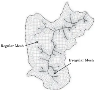
numerical model construction – cma module
figure 3. To create the finite element mesh, points coinciding with the contours were defined, spaced
at least 200 m from one another (Figure 3). Close to the wells and the rivers, the mesh has a variable,
refined spacing. The internal contours are the wells
and rivers, and the external borders is the watershed boundaries (Figure 3).
The initial potentiometric surface was created from the interpolation of the measured phreatic levels (Figure 4). Figure 4 shows the flow map in ROW, representing the element velocities by
vectors. The spatial velocity distribution confirms
the consistency of the model, once regions with unrealistic drainage values or drastic direction
changes were not identified (Figure 4). The map also shows boundary areas in which lateral flows were
considered in the aquifer.
Based on geological, hydrogeological and soil properties, as well as estimates of other GAS areas, presented by Sracek and Hirata (2002) and Gastmans and Kiang (2005), the initial value of
K = 4.32 m d-1 (5 × 10⁻⁵ m s-1) was adopted. This
initial estimate was modified throughout the calibration process and spatialized based on the pedological map of the area. The magnitude of the
final K values (1.3 × 10⁻⁶ to 2.6 × 10⁻⁵ m s-1) are in the order of the intervals found by Sracek and
Hirata (2002) (2 × 10⁻⁶ to 1.9 × 10⁻³ m s-1) in the
State of São Paulo.
Specific yield values obtained by Gomes (2008)
for the study area are between 8.5 and 15.9 %. These results are similar to the ones found by Sracek and Hirata (2002) for the GAS regions (7 a 15 %). To
specify the porosity, the influence areas specified
by Gomes (2008) were considered. They were obtained as a function of the average thickness of the unsaturated layer and the distance of the collection points from the water stream.
The attributions made to the RIOS field are
related to the representation of ranges, in which the aquifer surface is practically outcropping, and, in the rainy season, give rise to springs. In these parts with high evapotranspiration rates, the third boundary condition was applied.
This adjustment considered that the highly
elevated fixed potentials may cause, over time, a
rise in the levels (even without recharge increase), because they function as water sources of the
aquifer. Over time, very low fixed potentials result
in a lowering of the levels (also without alteration in recharge), since a high hydraulic gradient
Potential (m) (Hydraulic head) after 2586 days
640-650
650-660 660-670 670-680 680-690
690-700 700-710
710-720 720-730 730-740 740-750
750-760
760-770
Flow direction
figure 4. Potentiometric surface obtained after running the model. Vectors in black represent the darcy velocities.
Irregular Mesh Regular Mesh
figure 3. discretization of the model domain in a finite element mesh.
db = P - Etr - Es
db + Rsoil>Smax RP = db + Rsoil - Smax
Rsoil = Smax
R = Crec × Rp
Rsoilt+1 = Rsoilt + db
Se Rsoilt+1<0; Rsoil = 0
Se Rsoilt+1>0;
Rsoil = Rsoilt+1
Rsoilt+1 = Rsoilt + db
R = 0
db = P - Etr - Es P>Etr
opposite to the river flow is imposed, which begins
to function as a sink.
recharge estimation
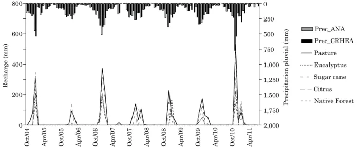
Recharge rates were calculated on a monthly scale, applying the water balance proposed in the methodology for different land use types (Figure 5). Total monthly rainfall registered at the
stations ANA and CRHEA are shown in figure 5.
Importantly, spatial variability in rainfall must not be ignored. Pedersen et al. (2010) observed significant differences (variation coefficient of up to 77 %) in an area of 0.25 km². Correlation values lower than 0.5 were found for rainfall series measured 10 km apart (Tokay et al., 2014).
Even at a distance of less than 10 km between
the stations ANA and CRHEA, there are significant
differences in some months, e.g., in January 2011, the pluviometer at ANA registered almost 100 mm more rain. These differences were detectable when
comparing the recharge results estimated by the water balance method and those presented by Lucas et al. (2012) on an annual scale.
The referred comparison is shown in figure 6,
where greatest differences are observed between the estimates for areas of pasture and plantation in 2009 (~100 mm) and 2010 (~120 mm), respectively. A possible explanation for these discrepancies is the spatial variability in rainfall. As shown by the weather station data for the study area, and by Tokay et al. (2014) and Pedersen et al. (2010), the totality of a given rainfall may not be recorded in areas close to the measuring site. Depending on the rainfall series used to generate the water balance (WB), substantially distinct recharge rates are found.
Differences between recharge values estimated by the methods WTF and WB can be explained by the uncertainty related to the input variables of the methods. In the case of WTF, an essential
parameter in the equation is the specific yield (Sy)
Recharge (mm)
700 600
400 500
200 300
100 0
2004/05
Hydrological year
2005/06 2006/07 2007/08 2008/09 2009/10 2010/11
Pasture_WB Pasture_WTF Sugar cane_WB Sugar cane_WTF Citrus_WB Citrus_WTF
figure 6. comparison between y the annual recharge rates obtained by the water Balance and water table fluctuation (wtf) methods.
0 250 500 750 1,000 1,250 1,500 1,750 2,000 0
200 400 600 800
Oct/0
4
A
pr/0
5
Oct/0
5
A
pr/0
6
Oct/06 Apr/0
7
Oct/07 Apr/0
8
Oct/08 Apr/0
9
Oct/09 Apr/1
0
Oct/10 Apr/1
1
Precipitation pluvial (mm)
Recharge (mm)
Prec_ANA Prec_CRHEA Pasture Eucalyptus Sugar cane Citrus Native Forest
related to soil porosity. This parameter is hard to determine and usually varies according to the depth, due to the heterogeneity of natural soils. In the case of WBM, the variable with greatest uncertainty is evapotranspiration (ET), whose definition depends on climatic variables and crop coefficients, adopted from values cited in the literature.
model calibration – tP module
The transient simulation of the model was made using module TP of SPA, and the distributed values of the monthly recharge rates estimated by the water balance as input (Figure 7). The results were stored on a monthly basis between 2004 and 2010 (0 to 2500 days). For each simulation, the software generated deviation reports. The average and maximum deviations computed for each node corresponding to the monitoring wells (Table 1).
The calibration was more difficult in the second
year of simulation, since the observed levels do practically not respond to the rainfall events, reaching a maximum difference of 1.80 m in relation to what is simulated in P13. For this node, the average error (0.59 m) was slightly higher to the one found for P14 (0.58 m). These differences can indicate that the recharge rates calculated for the respective periods are under or overestimated by the adopted method.
Despite the adjustments, the model is still a
simplification of the real processes and, therefore,
contains limitations which, in this study, could be
identified close to the boundary conditions. The node
referring to well 16 (P16) is found on the border between mesh elements that refer to the native forest and pasture.
In the rainy season, the aquifer level rises close to the surface or emerges to the marginal river areas. With this, losses by direct transpiration rise, and due to the complexity of their incorporation in the water balance to estimate the recharge, the model responds with a damming effect, expressed in peaks exceeding the observed values. Still, for the remaining period, the simulated are satisfactorily close to the measured levels, with an average error lower than 0.5 m in wells 16 and 17.
Table 1. Maximum and mean errors at the nodes used in the calibration of the numerical model for the ribeirão da onça watershed
node corresponding to well Error
Maximum average
m
05 0.95 0.32
13 1.80 0.59
14 1.53 0.58
15 1.30 0.39
16 1.34 0.31
17 1.35 0.47
18 2.29 0.93
19 3.05 0.95
742 744 746 748 750 752
Well 5
692 694 696 698 700 702
Well 15
698 700 702 704 706 708
Well 13
698 700 702 704 706
Well 14
0 1000 2000 702
704 706 708 710 712
Well 16
Level (m)
0 1000 2000 704
706 708 710 712 714
Time (day) Well 17
0 1000 2000 708
710 712 714 716 718
Well 18
0 1000 2000 712
714 716 718 720 722 696
Well 19 Simulated Observed
conclusions
Results of recharge estimated by water balance in the unsaturated soil zone were similar to the previously obtained by the WTF method. The differences between the estimates were lower than 50 mm in more than 60 % of the cases.
The greater differences between the BH and WTF responses are related to the intrinsic limitations of the methods, spatial variability of rainfall and uncertainties in the input data.
Although groundwater recharge cannot be directly measured to validate the estimates established indirectly by different methods (e.g.,
WTF or Water Balance), a similar verification or
comparison of the simulated to the measured levels
can be performed in loco using a numerical model
of transient flow.
The calibration of the numerical model evidenced
the influence of the most distinct hydrogeological
parameters, and reinforced the importance of compiling more spatial information to characterize the study area in greater detail, thus reducing uncertainties in modeling.
Computational models can be used not only to control the recharge estimates, but also to deepen the understanding of processes occurring in the study area, or even allow an evaluation of the impact of different climatic scenarios at the aquifer levels.
rEfErEncEs
Allen GR, Pereira LS, Raes D, Smith M. Crop Evapotranspiration (guidelines for computing crop water requirements). Rome: Food and Agriculture Organization of the United Nations; 1998. (FAO Irrigation and Drainage Paper, 56).
Araújo LM, França AB, Potter PE. Hydrogeology of the Mercosul aquifer system in the Paraná and Chaco-Paraná Basins, South America, and comparison with the Navajo-Nugget aquifer system, USA. Hydrogeol J. 1999;7:317-36.
Barrett R, Berry M, Chan TC, Demmel J, Donato J, Dongarra J, Eijkhout V, Pozo R, Romine C, van der Vorst H. Templates for the solution of linear systems: building blocks for iterative methods. 2nd.ed. Philadelphia [PA]: SIAM; 1994.
De Vries J, Simmers I. Groundwater recharge: an overview of processes and challenges. Hydrogeol J. 2002;10:5-17.
Gastmans D, Kiang CH, Hutcheon I. Stable isotopes (2H, 18O and 13C) in groundwaters from the northwestern portion of the Guarani Aquifer System (Brazil). Hydrogeol J. 2010;18:1497-513. Gastmans D, Kiang CH. Avaliação da hidrogeologia e hidroquímica do Sistema Aquífero Guarani (SAG) no estado do Mato Grosso do Sul. Águas Subt. 2005;19:35-48.
George PL, Seveno E. The advancing-front mesh generation method revisited. Int J Numer Meth Eng. 1994;37:3605-19.
Gomes LH. Determinação da recarga profunda na bacia-piloto do Ribeirão da Onça em zona de afloramento do Sistema Aquífero Guarani a partir de balanço hídrico em zona saturada [dissertação]. São Carlos: Universidade de São Paulo; 2008.
Healy R, Cook P. Using groundwater levels to estimate recharge. Hydrogeol J. 2002;10:91-109.
Healy RW, Winter TC, Labaugh JW, Franke O. Water budgets: foundations for effective water-resources and environmental management. Reston, Virginia: U.S. Geological Survey; 2007. (Circular, 1308).
Kwon HH, Souza Filho FA, Block P, Sun L, Lall U, Reis DS. Uncertainty assessment of hydrologic and climate forecast models in Northeastern Brazil. Hydrol Process. 2012;26:3875-85. Lucas MC, Guanabara RC, Wendland E. Estimating groundwater recharge in the outcrop area of the Guarani Aquifer System. B Geol Min. 2012;123:311-23.
Machado AR, Wendland E, Krause P. Improving water balance in an outcrop area of the Guarani Aquifer System through hydrologic simulation. Environ Process. 2014 (Submitted).
Manzione R, Tanikawa DH, Wendland E. Análise de tendências nos níveis freáticos de uma bacia hidrográfica em área de recarga
do Sistema Aquífero Guarani (SAG) auxiliado por imagens de sensoriamento remoto, sistemas de preparo de solo: alterações na estrutura do solo e rendimento das culturas. In: Anais do 15º Simpósio Brasileiro de Sensoriamento Remoto; 2011; São José dos Campos. São José dos Campos: INPE; 2011. p.1-17. Medeiros PV, Marcuzzo FFN, Youlton C, Wendland E. Error autocorrelation and linear regression for temperature-based evapotranspiration estimates improvement. J Am Water Res Assoc. 2012;48:297-305.
Melo DCD. Estimativa de impacto de mudanças climáticas nos níveis do aquífero livre em zona de recarga do Sistema Aquífero Guarani [dissertação]. São Carlos: Universidade de São Paulo, 2013.
Organização dos Estados Americanos - OEA. Programa Estratégico de Ação do Projeto de Proteção Ambiental e Desenvolvimento Sustentável do Sistema Aquífero Guarani [Relatório técnico]. 2009.
Pedersen L, Jensen NE, Christensen LE, Madsen H. Quantification
of the spatial variability of rainfall based on a dense network of rain gauges. Atmos Res. 2010;95:441-54.
Raneesh KY, Thampi S. A simple semi-distributed hydrological model to estimate groundwater recharge in a humid tropical basin. Water Res Manage. 2013;27:1517-32.
Rodríguez L, Vives L, Gomez A. Conceptual and numerical modeling approach of the Guarani Aquifer System. Hydrol Earth Syst Sci. 2013;17:295-314.
Scanlon BR, Healy R, Cook P. Choosing appropriate techniques for quantifying groundwater recharge. Hydrogeol J. 2002;10:347-21.
Scanlon BR, Keese KE, Flint AL, Flint LE, Gaye CB, Edmunds WM, Simmers I, Cook P. Global synthesis of groundwater recharge in semiarid and arid regions. Hydrol Process. 2006;20:3335-70.
Tokay A, Roche RJ, Bashor PG. An experimental study of spatial variability of rainfall. J Hydrometeor. 2014;15:801-12.
Wendland E, Barreto C, Gomes LH. Water balance in the Guarani Aquifer outcrop zone based on hydrogeologic monitoring. J Hydrol. 2007;342:261-9.
Wendland E, Gomes LH, Troeger U. Recharge contribution to the Guarani Aquifer System estimated from the water balance method in a representative watershed. An Acad Bras Ci. 2014;87:595-609.
Wendland E, Rabelo JL. Incertezas nos modelos de fluxo subterrâneo. R Bras Rec Hídric. 2010;15:147-60.
Wendland E, Simonato MD, Lapiccirella ES, Hirata R. Modelo numérico de escoamento subterrâneo na região de São José do Rio Preto, São Paulo-SP. Águas Subt. 2013;27:92-109.