Soccol & Botrel 134
HYDROCYCLONE FOR PRE-FILTERING
OF IRRIGATION WATER
Olívio José Soccol1; Tarlei Arriel Botrel2*
1
UDESC/CAV - Depto. de Engenharia Rural, C.P 281 - 88520-000 - Lages, SC - Brasil. 2
USP/ESALQ - Depto. de Engenharia Rural, C.P 09 - 13418-900 - Piracicaba, SP - Brasil. *Corresponding author <[email protected]>
ABSTRACT: The use of water containing suspended sediments causes serious problems to irrigation systems. Choosing the right filtering system type and capacity is essential to avoid increases in operational and maintenance costs of irrigation resulting from the need for cleaning and frequent component replacing. Pre-filters, such as the hydrocyclone, are important for their significant capability of retaining particles suspended in the water. Data on hydrocyclones performance for pre-filtering of irrigation water can be found in the literature, but research data in Brazil are scarce. Therefore, four Rietema type hydrocyclones (50 mm diameter) were constructed, one with circular-end and the other three presenting rectangular-end feeding tubes. The evaluation of hydrocyclones performance was conducted by using suspensions of fine sand and clay soil particles under varied pressure differentials. The comparison criteria were the discharge and the separation capability, given by total efficiency and reduced total efficiency. The hydrocyclone with circular-end feeding tube presented the highest indexes for the adopted criteria, considering sand and soil suspensions.
Key words: filtration, cyclones, centrifugal separator
HIDROCICLONE PARA PRÉ-FILTRAGEM DA
ÁGUA DE IRRIGAÇÃO
RESUMO: A utilização de água contendo partículas sólidas em suspensão tem sido a causa de sérios problemas em sistemas de irrigação. A escolha do tipo e capacidade do sistema de filtragem é de fundamental importância para evitar aumento nos custos de operação e manutenção do sistema de irrigação. Pré-filtros, como os hidrociclones, caracterizam-se por significativo poder de separação de partículas presentes na água. Apesar de algumas referências feitas aos hidrociclones, não se dispõe no Brasil de resultados do desempenho dos mesmos, quando empregados em pré-filtragem da água utilizada nos sistemas de irrigação. Assim, um experimento compreendeu a construção e a avaliação do desempenho de quatro hidrociclones do tipo Rietema, utilizando-se suspensões de areia fina e de solo argiloso, sob diferentes diferenciais de pressão, e adotando-se como critério de comparação a capacidade de vazão e o poder de adotando-separação, medidos pela eficiência total e eficiência total reduzida. O hidrociclone dotado com bocal de alimentação circular apresentou os maiores índices nos critérios de comparação, com suspensão de areia e suspensão de solo.
Palavras-chave: filtração, ciclones, separador centrífugo
INTRODUCTION
Sediments present in the water usually reduce du-rability of irrigation system components such as pump ro-tors, feeding tubes and localized irrigation pipelines. Sedi-mentation basins and hydrocyclones can be used to re-duce the size and costs of filtering systems (Keller & Bliesner, 1990).
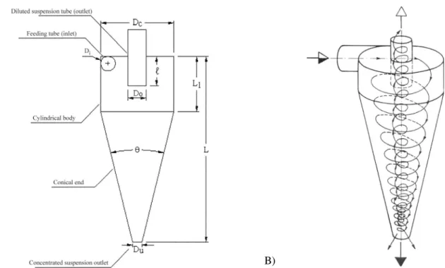
The hydrocyclones are an important class of equipments destined to separation of solid-liquid suspen-sion phases (Souza et al., 2000). An hydrocyclone con-sists of a conic end linked to a cylindrical body, in which there is a tangential entrance for the feeding suspension. The hydrocyclone has a tube in its upper part for the di-luted suspension draining (overflow) and a hole in the un-der part for the concentrated suspension draining (unun-der- (under-flow) (Figure 1 a). The suspension is pumped through the
feeding tube and when entering the hydrocyclone it is ac-tivated by a rotational, descendent movement and tends towards the drainage point of the underflow (Flintoff et al., 1987) as shown in Figure 1b.
When the feeding suspension is introduced into the hydrocyclone, a fraction of the liquid and the higher velocity (heavier) particles are discharged through the concentrated underflow drain. The remaining liquid and the lower velocity (lighter) particles are discharged throughout the diluted overflow drain (Silva, 1989). Even though the hydrocyclone may not be separating by cen-trifugation, a certain amount of solids is removed with the concentrated in a rate that may be defined by the equa-tion:
(
)
(
Cv
)
Q
Cv
Q
R
L u u−
−
=
1
1
where: RL – liquid ratio, non-dimensional; Qu – concen-trated suspension outflow, L T-1; Q – feeding suspension
outflow, L3 T-1; Cv
u – volumetric concentration of the
con-centrated suspension, non-dimensional; Cv - volumetric concentration of the feeding suspension, non-dimensional (Silva, 1989).
The total or global efficiency is defined as the ratio between the concentrated suspension solid mass outflow and the feeding suspension solid mass out-flow:
Ws Ws
E u
T = (2)
where: ET – total efficiency, non-dimensional; Ws - feed-ing suspension solid mass flow, M T-1; Ws
u - concentrated
suspension solid mass flow, M T-1.
The reduced total efficiency is calculated by sub-tracting the “dead flow” contribution, thus resulting in the hydrocyclone actual performance, which has been calcu-lated by the expression:
L L T T
R
R
E
E
−
−
=
1
'
(3)
where: E’T – reduced total efficiency, non-dimensional; ET – total efficiency, non-dimensional; RL – liquid ratio, non-dimensional (Kelsall, 1953).
This work aimed to construct and evaluate four hydrocyclones with equal dimensions, but varying the
form and dimension of the feeding tubes, operating with sand and soil suspensions, in order to obtain best perfor-mance parameters and efficiency on the removal of solid particles present in the water.
MATERIAL AND METHODS
Hydrocyclone assembly
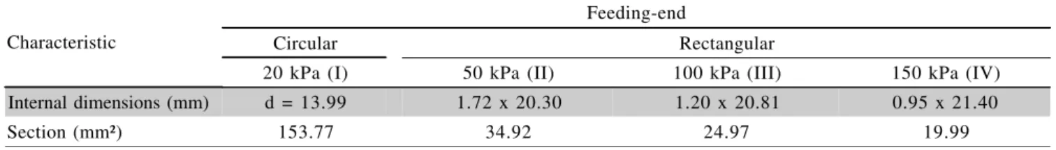
Four 50 mm-diameter hydrocyclones were as-sembled for the experiment. Equipment dimensions fol-lowed recommendations of Rietema (1961), differing only regarding the shape and dimensions of the feeding tube. The hydrocyclone with circular-end feeding tube, Hydrocyclone I, the first to be dimensioned, had 13.99 mm internal diameter. The other three hydrocyclones were assembled with rectangular-end feeding tubes with different shapes and sizes (Table 1). For the circular-end feeding tube, the inflow rate established was equal to 2 m s-1, and the outflow, defined by the continuity
equa-tion, was 0.31 L s-1. Dimensions of the retangular-end
feeding tube were calculated considering hydrocyclone pressure reduction of 50, 100 and 150 kPa, for hydrocyclones II, III and IV, respectively, using the con-tinuity equation and an average discharge coefficient of convergent, conical-end feeding tube equal to 90% (Neves, 1979).
The feeding tubes were assembled using 15-mm nominal diameter (ND), commercial copper tubes, and the rectangular-ends were molded with the correspondent di-mensions (Table 1).
A) B)
Figure 1 - Diagram showing the main hydrocyclone dimensions (a) and the internal draining movement (b).
DC – Hydrocyclone diameter; Di – feeding tube diameter; Do – diluted overflow tube diameter; DU – concentrated underflow tube diameter; L – hydrocyclone length; l - diluted overflow tube reentrance; L
Soccol & Botrel 136
Essay material
Fine sand and clayey-soil were used as sediment material (Kandiudalfic Eutrudox). After rinsing the fine sand, was sieved through a 1.19 mm screen to remove coarse particles. The soil was sieved through a 0.54 mm screen to remove small gravels. Density of sand and soil particles were determined by the Pycnometer (density bottle) method (Kiehl, 1979), resulting in values of 2.65 g cm-³ and 2.70 g cm-³, for sand and soil,
respec-tively. Soil fractions were also determined according to Kiehl (1979), and the following values were found: 73.55% clay, 18.26% silt, and 8.19% sand.
Experimental workbench
The experiment was performed in a workbench, in closed circuit (Figure 2):
1) Reservoir: For the sand-water or soil-water suspen-sions, 500 L capacity.
2) Motor-pump: Centrifugal pump with discharge flow of 4,500 L h-1 (0.00125 m³ s-1), pumping pressure of 340
kPa, and electrical motor with 1,470.60 W (2 HP) and 3,500 rpm.
3) Flowmeter: Electromagnetic flowmeter with nominal flow of 1,000 L h-1 (0,000278 m³ s-1).
4) Pressure sensor: The pressure-differential in the hydrocyclone was evaluated by pressure plugs installed into the feeding tube and diluted suspension, using
dif-ferential-transducer pressure sensors with capacity within the range of 0 to 700 kPa and 2.5% error for temperatures between 0 and 85oC. When fed by a 5V c/c stabilized
ten-sion, the sensor emits analogical signals varying from 0.2 to 4.7V c/c, which are transformed in pressure readings. The pressure-transducer outputs were also linked to the digital analogical converser (DAC), allowing monitoring of the pressure reduction in the hydrocyclone.
5) Hydrocyclone: Sampling sites were installed close to the hydrocyclone, in the feeding tube (a) and in the di-luted suspension (b).
6) Submersible shaker: Electrical motor, 1,102.90 W (1,5 HP) and 1,650 rpm, kept suspension homogeneous during samplings.
7) Microcomputer: Equipped with the software Aquidados (Vilela et al., 2001), to control the digital ana-logical converter by signals emitted through the computer parallel port. The software also controlled transmission of digital data to the CPU unity. Such information was processed and displayed in the video-monitor, at real time, and results were simultaneously stored in specific files, with respective reading date and time records.
Experimental procedures
Sand and soil suspensions were prepared by the addition of 20 kg of material, previously sieved, to 450 L of water, resulting in an initial sediments concentration of 44.44 g L-1
.
Table 1 - Characteristics of the feeding tubes used in the hydrocyclones.
Characteristic
Feeding-end
Circular Rectangular
20 kPa (I) 50 kPa (II) 100 kPa (III) 150 kPa (IV)
Internal dimensions (mm) d = 13.99 1.72 x 20.30 1.20 x 20.81 0.95 x 21.40
Section (mm²) 153.77 34.92 24.97 19.99
Figure 2 - Diagram of the experimental workbench and components.
(7)
(2)
(a)
(4) (b)
(5)
(6)
(3)
Starting of system: The workbench system was set in motion by the motor-pump; the microcomputer, the flow-meter, the pressure-sensor and the submersible shaking were then turned on. The desired pressure reduction was adjusted by the software through a gate valve installed in the pump output. Pressure differentials were: 10, 20, 30, 40, 50, and 60 kPa, for the hydrocyclone I, operating with sand and soil suspensions; 20, 50, 100, and 150 kPa, for hydrocyclones II, III and IV, operating with soil sus-pension. After systems reached equilibrium, the tempera-ture of the suspension was checked and data monitoring started. The liquid ratio (LR) was adjusted to 10% by the gate valve installed in the output of the concentrated sus-pension.
Data monitoring: The reading interval and data registra-tion period were adjusted to 60 s in the initial display screen, and then the reading key was entered. During the flow and pressure reduction data-collecting period, aliquot samples of the concentrated suspension were taken at 30 s intervals and weighed, to obtain the sample mass. When the flow and pressure differential readings were finished, the feeding suspension sampling started. This procedure was repeated for each pressure differential point sampled.
Concentration measurements: The sample concentra-tions were determined using the gravimetric method. An aliquot sample (exact volume) was transferred to an alu-minum recipient and oven dried at 110oC for 24 hours.
After evaporation, the residue was weighed for dry mat-ter demat-termination and expressed as g L-1.
Analysis of particle size fraction: The determination of sand and soil particle size fraction followed distinct pro-cedures, since the replications of each sample were pooled, due to small quantity of solids collected, mainly from the feeding flow. Determination of the sand frac-tion was done by the sieve method and determinafrac-tion of the soil fraction, by the sedimentation method (Allen, 1990). A kit of ten sieves, mesh 1,000, 590, 500, 420, 297, 250, 149, 105, 74, and 53 mm was used for the sand fraction analysis. The total amount of dry sand was weighed and three subsamples were taken; each subsample was set top the kit and sieved by shaking for 12 minutes. Sieves were then weighed to obtain the frac-tion mass (X), correspondent to each screen meshes.
For determination of the soil particle size frac-tion, the method used was based on the gravimetric sedi-mentation, and the variation on the sediment concentra-tion of the collected samples at determined intervals, al-lowed to calculate the cumulative fraction, in a mass ba-sis, lower than a certain diameter (d), determined by the Stoke´s law. The dried soil sample was weighed and transferred to a recipient with distilled water, let stand for 24 hours and stirred at 16,000 rpm for 20 minutes to disaggregate the particles. The suspension was then
transferred to a 1,000-mL graduated cylinder, distilled water was added until completing the volume, and the suspension was manually stirred for 60 seconds, using a plain-disc. The sampling period was then started: 10-mL samples were taken, using a pipette plunged 10 cm into the suspension, after 10, 30, 60, 120, 180, 300, 600, 1,200, and 1,800 seconds. Samples were transferred to small vials and oven-dried at 110oC for 24 hours. The
dry residue was weighed in analytical balance to the nearest 0.0001 g, for the determination of mass fraction X lower than a certain Stokes diameter, using the Equa-tion (4):
o
C
C
X
=
(4)where: X – mass fraction lower than a certain diameter, non-dimensional; C – sample concentration collected at time t, M L-1; C
o – initial concentration, M L -1.
At the beginning of each essay, the suspension’s temperature was monitored in the graduated cylinder. The correspondent Stokes’ diameter was calculated by Equa-tion (5), for each defined sampling period of time, and resulted approximately in 7, 8, 12, 17, 22, 27, 38, 54, and 93 mm, respectively.
(
)
5 , 018
−
=
ρ
ρ
µ
s tkgt
h
ds
(5)where: dstk - Stokes’ diameter, L; m - fluid absolute vis-cosity, M L-1 T-1; h – pipette sampling depth, L; g –
ac-celeration due to gravity, L T-2
; t – sampling time inter-val, T; ρs – solid density, M L-3; ρ - fluid density, M L-3.
RESULTS AND DISCUSSION
Hydrocyclones performance Hydrocyclone I
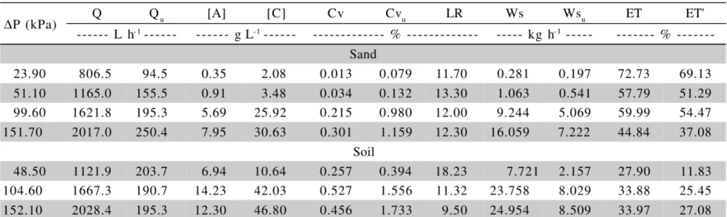
Mean values on hydrocyclone I performance op-erating with sand and soil suspension are presented in Table 2. The suspension sediment concentration varied with increasing pressure differential. It was not possible to keep the suspension homogeneous in the input flow to the centrifugal pump at the same time that the work-bench dynamic conditions were altered, since the stirring velocity of submersible shaker was at the limit above which the suspension started to be ejected out of the res-ervoir. As no other shaker was available, the test took into account differences in suspension concentrations.
The feeding flow varied from 1,159.9 L h-1 to
2,603.6 L h-1 and from 1,160.9 L h-1 to 2,534.8 L h-1, for
operation with sand and soil suspension respectively. The suspension temperature remained between 21oC and 22oC
Soccol & Botrel 138
For the sand suspension essays, the highest in-dices of total reduced efficiency ET’ were 94.45% and 96.62%, obtained for pressure differences of 10.80 kPa and 22.30 kPa, respectively; the lowest was 64.61% for a 62.70 kPa difference. For the soil suspension essays, ET’ varied from 14.38% to 38.19% for pressure differences of 11.90 kPa and 43.50 kPa, respectively, decreasing to 31.94% for a 63.60 kPa pressure differ-ence.
When operating with sand, hydrocyclone I had al-ways higher total reduced efficiency ET’ for similar pres-sure differences, as expected, due to the sand particle size characteristics. The average ET’, for all the pressure dif-ferences, was 80.13% and 30.87% for the sand and soil tests, respectively. The hydrocyclone separation capacity depends on its size and geometry, particle size and ge-ometry, solid concentration, inflow rate, liquid ratio and density difference between particles and fluid (Jacobs & Penney, 1987). The highest sand suspension concentra-tions, for pressure differences higher than 22.30 kPa, had no effect on hydrocyclone performance. Even for higher feeding flows there was no gain in efficiency, what might be consequence of a greater turbulence into the hydrocyclone. For the soil suspension, the lower efficien-cies obtained may be explained by the smaller particle sizes.
Hydrocyclones II, III and IV
Significantly lower feeding suspension concentra-tions in hydrocyclones II, III and IV were observed in comparison to those in hydrocyclone I, mainly for the
pressure differences of 20 kPa and 50 kPa (Tables 3, 4 and 5), what may be explained by a lower feeding flow and, consequently, lower suspension turbulence in the res-ervoir, for first ones. The feeding flows observed during the tests varied from 806.5 L h-1 to 2,028.4 L h-1,
401.3 L h-1 to 1,095.3 L h-1 and 322.8 L h-1 to 847.7 L h-1
for hydrocyclones II, III and IV, respectively.
The reduced total efficiencies obtained for hydrocyclones II, III and IV were similar to the hydrocyclone I, and the highest values were observed in the sand suspension test, with the following average mean values, for all pressure differentials: hydrocyclone II -52.99% and 21,45% for sand and soil suspension, respec-tively; hydrocyclone III – 36.69% and 17.25% for sand and soil suspension, respectively; hydrocyclone IV – 34.45% and 12.66% for sand and soil suspension, respec-tively.
Comparing the performance of the four hydrocyclones, using ET’ as reference, and considering a common pressure differential of 50 kPa, decreasing flows were observed for the hydrocyclones II, III and IV of 51.04%, 73.92% and 78.38%, respectively, in relation to the hydrocyclone I. The flow reduction did not repre-sent efficiency gains for these hydrocyclones, meaning that, at the same test conditions, the reduced total effi-ciency decreased 26.72%, 53.98% and 38.52% for the sand suspension, and 62.60%, 71.04% and 78.69% for the soil suspension, for hydrocyclones II, III and IV, respec-tively. Hydrocyclones III and IV showed feeding tube ob-struction, what might be explained by the smaller feed-ing tube diameter (Table 1).
∆P (kPa) Q Qu [A] [C] Cv Cvu LR Ws Wsu ET ET'
--- L h-1 --- --- g L-1 --- --- % --- --- kg h-1 --- %
---Sand
10.80 1159.9 133.5 2.81 23.26 0.106 0.879 11.42 3.265 3.104 95.08 94.45 22.30 1582.8 223.3 2.99 21.09 0.113 0.797 13.66 4.849 4.708 97.09 96.62 29.50 1826.8 133.7 6.19 69.34 0.234 2.627 7.14 11.314 9.269 81.93 80.54 40.40 2002.2 207.6 6.11 45.50 0.231 2.720 10.22 12.239 9.444 77.16 74.56 52.00 2386.2 249.4 5.93 42.99 0.224 1.625 10.25 14.139 10.273 72.79 69.99 62.70 2603.6 259.2 7.01 47.95 0.265 1.813 9.80 18.255 12.427 68.07 64.61
Soil
11.90 1160.9 156.5 7.29 13.98 0.270 0.518 13.48 8.436 2.188 25.93 14.38 22.60 1595.1 143.9 11.46 51.10 0.424 1.893 8.89 18.279 7.356 40.29 34.46 29.60 1813.8 141.5 11.32 58.03 0.419 2.149 7.69 20.542 8.141 39.63 34.62 43.50 2128.9 201.2 11.10 51.68 0.411 1.914 9.31 23.643 10.403 43.94 38.19 51.90 2284.8 220.4 10.89 43.07 0.403 1.595 9.53 24.383 9.497 38.15 31.63 63.60 2534.8 244.7 12.12 48.24 0.449 1.787 9.52 30.727 11.796 38.42 31.94
Table 2 - Average data of performance parameters of Hydrocyclone I operating with sand and soil suspension.
Total efficiency
The reduced total efficiency excludes the “dead flow” effect present in the hydrocyclones, that is, there is a minimal separation efficiency because part of the
feeding flow escapes the hydrocyclone by the concen-trated duct. Such procedure allows performance analysis without taking into account the liquid ratio, which showed a variation among the tests in consequence of the particle Table 5 - Average data of performance parameters of Hydrocyclone IV operating with sand and soil suspension.
∆P (kPa) Q Qu [A] [C] Cv Cvu LR Ws Wsu ET ET'
--- L h-1 --- --- g L-1 --- --- % --- --- kg h- 1 --- %
---Sand
28.00 322.8 39.6 0.02 0.04 0.001 0.002 12.30 0.007 0.002 24.76 14.25 54.90 497.6 51.3 0.35 1.67 0.013 0.063 10.30 0.174 0.086 49.26 43.03 101.00 631.9 72.1 1.62 6.77 0.061 0.256 11.40 1.024 0.489 47.72 41.00 148.80 829.9 91.5 11.87 49.60 0.449 1.875 10.90 9.848 4.537 46.07 39.50
Soil
52.40 512.4 111.6 5.93 7.36 0.220 0.273 21.78 3.037 0.822 27.05 6.74 105.50 652.7 139.9 8.54 12.86 0.316 0.476 21.40 5.571 1.798 32.28 13.84 149.60 847.7 151.1 9.67 17.40 0.358 0.644 17.78 8.199 2.629 32.08 17.40
∆P – pressure differential in the hydrocyclone; Q – feeding flow; Qu – concentrated flow; [A] – feeding solid concentration; [C] – concentrated suspension solid concentration; Cv – feeding volumetric concentration; Cvu – concentrated volumetric concentration; LR – liquid ratio; Ws – feeding solid mass flow; Wsu – concentrated solid mass flow; ET – total efficiency; ET’ – reduced total efficiency.
Table 4 - Average data of performance parameters of Hydrocyclone III operating with sand and soil suspension.
∆P – pressure differential in the hydrocyclone; Q – feeding flow; Qu – concentrated flow; [A] – feeding solid concentration; [C] – concentrated suspension solid concentration; Cv – feeding volumetric concentration; Cvu – concentrated volumetric concentration; RL – liquid ratio; Ws – feeding solid mass flow; Wsu – concentrated solid mass flow; ET – total efficiency; ET’ – reduced total efficiency.
∆P (kPa) Q Qu [A] [C] Cv Cvu RL Ws Wsu ET ET'
--- L h-1 --- --- g L-1 --- --- % --- --- kg h- 1 --- %
---Sand
23.90 401.3 53.0 0.11 0.35 0.004 0.013 13.10 0.042 0.019 43.86 35.46 54.30 602.9 92.8 0.18 0.50 0.007 0.019 15.40 0.108 0.046 42.64 32.21 102.20 842.6 122.6 0.40 1.16 0.015 0.044 14.50 0.339 0.143 42.09 32.23 151.10 1012.9 100.3 3.42 18.01 0.295 0.681 9.80 3.468 1.806 52.07 46.84
Soil
48.90 615.4 113.1 7.37 10.05 0.273 0.372 18.36 4.491 1.141 25.84 9.16 104.20 891.6 116.6 5.75 14.69 0.213 0.544 13.04 5.169 1.708 34.25 24.40 152.00 1095.3 133.9 16.44 37.83 0.609 1.401 12.13 18.004 5.062 28.13 18.20
Table 3 - Average data of performance parameters of Hydrocyclone II operating with sand and soil suspension.
∆P – pressure differential in the hydrocyclone; Q – feeding flow; Qu – concentrated flow; [A] – feeding solid concentration; [C] – concentrated suspension solid concentration; Cv – feeding volumetric concentration; Cvu – concentrated volumetric concentration; LR – liquid ratio; Ws – feeding solid mass flow; Wsu – concentrated solid mass flow; ET – total efficiency; ET’ – reduced total efficiency.
∆P (kPa) Q Qu [A] [C] Cv Cvu LR Ws Wsu ET ET'
--- L h-1 --- --- g L-1 --- --- % --- --- kg h-1 --- %
---Sand
23.90 806.5 94.5 0.35 2.08 0.013 0.079 11.70 0.281 0.197 72.73 69.13 51.10 1165.0 155.5 0.91 3.48 0.034 0.132 13.30 1.063 0.541 57.79 51.29 99.60 1621.8 195.3 5.69 25.92 0.215 0.980 12.00 9.244 5.069 59.99 54.47 151.70 2017.0 250.4 7.95 30.63 0.301 1.159 12.30 16.059 7.222 44.84 37.08
Soil
Soccol & Botrel 140
separation by the centrifugal force. For practical purposes the main interest in the use of hydrocyclones as water pre-filtering for irrigation, is the potential of removal of par-ticles in suspension. Table 6 presents the average mean values for the total efficiency calculated from all the to-tal efficiencies observed for each pressure differential used in the essays, and for the average pressure differen-tial and the correspondent average feeding flow. Data in Table 6 represent the general behavior of each hydrocyclone, concerning separation potential power and the pressure differential necessary for best performance. In relation to the sand suspension tests, the highest effi-ciency value was obtained for the hydrocyclone I (82.02%), followed by lower values of 58.84%, 45.17%, and 41.95%, obtained for hydrocyclones II, III and IV, respectively. In the soil suspension tests, the highest ef-ficiency was also obtained for the hydrocyclone I, with reduction 1/3 of the pressure differential. However, lower differences in efficiency with the other three hydrocyclones were observed.
The increasing pressure differential in the rect-angular-end feeding tube hydrocyclones did not result in increased efficiency, but in lowering flows with conse-quent decreasing centrifugal forces generated in them. This evidenced the lower power of separation of these hydrocyclones when compared to the circular-end feed-ing tube hydrocyclone.
Although the tests were done with a high solid concentration in the suspensions, the hydrocyclones showed high performance, especially the hydrocyclone I, what demonstrates their relevance to the pre-filtering of water to be used for irrigation. Data presented in Table 6 show that, 4,732.6 g of sand could enter the system through irrigation during 1-hour operation without the help of a hydrocyclone; when a hydrocyclone is in op-eration, only 137.7 g 34.4-fold less of sand would enter the system, considering a homogeneous suspension. In another words, the irrigation system operating with the hydrocyclone I would take 34.4 hours to release the same amount of sand than released by an irrigation system in 1-hour without the hydrocyclone I. Test analysis with soil suspensions. Shows that 23,630.8 g and 13,248.1 g (1.78-fold less soil sediment) would be released from the sys-tem without and with the use of hydrocyclone I, respec-tively.
REFERENCES
ALLEN, T. Particle size measurement. 4.ed. London: Chapman & Hall, 1990. 832p.
FLINTOFF, B.C.; PLITT, L.R.; TURAK, A.A. Cyclone modeling: a review of present technology. Canadian Institute of Mining, Metallurgy and Petroleum Bulletin, v.80, p.39-50, 1987.
JACOBS, L.J.; PENNEY, W.R. Phase segregation. In: ROUSSEAU, R.W. (Ed.) Handbook of separation process technology. New York: Wiley-Interscience, 1987. cap.3, p.160-218.
KELLER, J.; BLIESNER, R.D. Sprinkle and trickle irrigation. New York: Chapman & Hall, 1990. 625p.
KELSALL, D.F. A further study of the hydraulic cyclone. Chemical Engineering Science, v.2, p.254-272, 1953.
KIEHL, E.J. Manual de edafologia: relações solo-planta. São Paulo: Ed. Agronômica Ceres, 1979. 264p.
NEVES, E.T. Curso de hidráulica. 6.ed. Porto Alegre: Editora Globo, 1979. 577p.
RIETEMA, K. Performance and design of hydrocyclones I, II, III, IV. Chemical Engineering Science, v.15, p.298-325, 1961.
SILVA, M.A.P. da. Hidrociclones de Bradley: dimensionamento e análise de desempenho. Rio de Janeiro: UFRJ, 1989. 81p. (Dissertação -Mestrado).
SOUZA, F.J.; VIEIRA, L.G.M.; DAMASCENO, J.J.R.; BARROZO, M.A.S. Analysis of the influence of the filtering medium on the behaviour of the filtering hydrocyclones. Powder Technology, v.117, p.259-267, 2000.
VILELA, L.A.A.; GERVÁSIO, E.S.; SOCCOL, O.J.; BOTREL, T.A. Sistema para aquisição de dados de pressão e vazão usando microcomputador. Revista Brasileira de Agrocomputação, v.1, p.25-30, 2001.
Hydrocyclone Suspension % kPa Q (L h- 1)
I sand 82.02 36.28 1926.92
soil 37.73 37.23 1919.72
II sand 58.84 81.58 1402.58
soil 31.92 101.73 1605.87
III sand 45.17 82.88 714.93
soil 29.41 101.70 867.43
IV sand 41.95 83.18 570.55
soil 30.47 102.50 670.93
Table 6 - Mean values of total efficiency, pressure differential and feeding flow calculated from the results of all tests made with the hydrocyclones operating with the sand and soil suspensions.
ET- average total efficiency of all tests; ∆P - average pressure differential of all tests; Q – feeding flow.
ET ∆P