MODELLING AIR TEMPERATURE FOR THE STATE OF
SÃO PAULO, BRAZIL
Luis Rodríguez-Lado1*; Gerd Sparovek2; Pablo Vidal-Torrado2; Durval Dourado-Neto3; Felipe Macías-Vázquez1
1
USC/Instituto de Investigaciones Tecnológicas - Lab. de Tecnología Ambiental - Campus Sur - Santiago de Compostela - 15782 - Spain.
2
USP/ESALQ - Depto. de Ciência do Solo, C.P. 09 - 13418-900 - Piracicaba, SP - Brasil. 3
USP/ESALQ - Depto. de Produção Vegetal. *Corresponding author <[email protected]>
ABSTRACT: Spatial modelling of air temperature (maximum, mean and minimum) of the State of São Paulo (Brazil) was calculated by multiple regression analysis and ordinary kriging. Climatic data (mean values of five or more years) were obtained from 256 meteorological stations distributed uniformly over the State. The correlation between the climatic dependent variables, with latitude and altitude as independent variables was significant and could explain most of the spatial variability. The coefficients of determination (P < 0.05) varied in the range of 0.924 and 0.953, showing that multiple regression analysis is an accurate method for the modelling of air temperature for the State of São Paulo. Finally, these regression equations were used together with the kriged maps of the residual errors to build 15 digital maps of air temperature using a 0.5 km2 Digital Elevation Model in a Geographic Information System.
Key words: DEM, GIS, multiple regression analysis, kriging, climate modelling
MODELAGEM DA TEMPERATURA DO AR PARA O
ESTADO DE SÃO PAULO, BRASIL
RESUMO: Foram utilizadas técnicas de análise de regressão linear múltipla e krigagem ordinária para a modelagem espacial das temperaturas máximas, mínimas, médias do Estado de São Paulo (Brasil). Os dados climáticos foram obtidos de 256 estações climatológicas distribuídas na totalidade do Estado. O período mínimo das séries climáticas utilizadas foi de cinco anos. Os resultados das análises de regressão apresentaram uma boa correlação entre as variáveis dependentes analisadas (temperaturas médias, máximas e mínimas) com a latitude, e a altitude como variáveis independentes. Os coeficientes de determinação (P < 0,05) variam entre 0,924 e 0,953 indicando que a regressão múltipla é um método preciso de estimativa da temperatura do ar no Estado de São Paulo. As equações de regressão obtidas foram utilizadas, em conjunto com mapas dos resíduos interpolados por krigagem, para a elaboração de 15 mapas de temperatura do ar sobre um modelo de elevação digital de 0,5 km2 de resolução espacial com a ajuda de geoprocessamento.
Palavras-chave: DEM, SIG, regressão linear múltipla, krigagem, modelagem climática
INTRODUCTION
Knowledge of the spatial distribution of cli-matic data is an essential tool for the management of natural resources and the prediction of climatic data is very useful in a wide number of scientific disci-plines (e.g.: agronomy, geography, and ecology). Moreover, the impact of fossil fuel burning and deforestation on climatic change raised the awareness for the development of adequate and reli-able prediction models of air temperature around the world.
Climatic data are usually measured in local meteorological stations. Climatic maps, covering
co-Kriging (Goovaerts, 2000) are frequently used. Mul-tiple regression analysis is another method widely used to compute the distribution of climatic variables from discrete data (Collins & Bolstad, 1996; Goodale et al., 1998; Ninyerola, 2000; Ninyerola et al., 2000; Lennon & Turner, 1995; Valeriano & Picini, 2000; Silva et al., 2006).
The objective of this study were i) to calcu-late spatial models of both monthly and annual air tem-peratures (mean, minimum and maximum) for the State of São Paulo (Brazil) using multiple regression analysis and ordinary kriging; ii) to use these models to derive digital raster maps of air temperature for the study area.
CASE STUDY
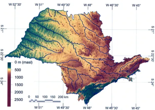
The State of São Paulo is located in the south-ern hemisphere (19-25º S, 44-53ºW) in Brazil, with an area of 248,816 km2. The State is divided into five geomorphologic units (Figure 1). The Western Pla-teau constitutes the main unit (60% of the area). Sedimentary deposits form this plateau and its mor-phology is dominated by flat to undulated landscapes of low hills with slopes between 0-20% (Cacheiro-Pose et al., 2002), and altitudes ranging between 250-650 m a.s.l. The Basaltic Cuestas spread from SW to NE in the middle of the State forming a range of trapps with alternating layers of basaltic rocks and eolian sandstones with altitudes between 500-900 m a.s.l. The Peripherical Depression, situated in the cen-tral portion of the State, constitutes a zone topo-graphically lower between the Basaltic Cuestas and
the Atlantic Region, with sediments, including shales, siltstones, sandstones and occasional basaltic intrusions. The Atlantic Region is the most elevated area formed by a plateau and two mountainous regions (Serra do Mar and Serra da Mantiqueira) with steep slopes between 0-20% in the plateau and from 10-40% in the mountains. It is formed mainly by igneous and metamorphic rocks, with altitudes ranging between 650-800 m a.s.l. in the plateau and up to 2703 m a.s.l. in the mountain ranges. These mountainous chains act as topographic barriers for oceanic fronts, therefore an important annual rainfall gradient is found between both sides of the ranges. The Coastal Region is a flat area along the coastal line narrowing on the direction SW-NE, where the ranges of the “Serra do Mar” come closer to the sea-coast.
The predominant climatic type in São Paulo is the tropical moist with dry winter (Aw) but the moist with mild winter climates with dry winter and hot (Cwa) and humid and hot (Cfa) according to Köppen’s classification are also frequent. Mean temperatures are smooth, ranging from 4.7-23ºC in winter and up to 29ºC in summer. Mean annual precipitation ranges from 1,350 to 1,550 mm. Rainy season occurs during October-March, coincid-ing with the higher temperature values (austral sum-mer). The dry season starts in April and ends in Oc-tober.
A total of 256 stations recording air tempera-ture were utilized in these analyses (CIIAGRO
base). The temperature data available from the CIIAGRO database had records ranging from 5 to 15 years. According to the World Meteorological Orga-nization (WMO, 1967), to ensure the optimal climate modelling, data series should extend to at least 30 years long. Such long time series are often unavail-able. However good results have also been obtained using shorter time series (Wotling et al., 2000; Marquinez et al., 2003).
Multiple regression analysis was used, com-bined with ordinary kriging, for air temperature mod-elling. The mean values of the climatic variables were considered as dependent variables in the multiple re-gression analysis. As possible independent variables nominal altitude (ALT), latitude (LAT) and longitude (LON) of the meteorological stations were consid-ered.
The adjusted regression model finally gives an expression in the form:
y = E0 + b1(X1) + b2(X2) +…+ bn(Xn) + ε (1)
where y is the estimated value of the dependent vari-able, E0 is the intercept, bnare multiple regression co-efficients, Xnthe significant independent variables and
ε is the residual error of the estimation.
For each model, the multiple coefficient of de-termination (R2) was computed, the multiple regres-sion coefficients building the model equation and the level of significance for each independent variable are also shown. Regression analyses were made using the stepwise method with inclusion of variables. Only in-dependent variables with a level of significance greater than 95% were accepted to build up the model.
These regression equations were converted to air temperature maps using map algebra with a Geographic Information System (ArcGIS 8.3), processing the independent variables as map layers in raster format. Altitude raster layer, in meters, was obtained from a 0.5 km2 Digital Eleva-tion Model (DEM) of the State (GTOPO30, 1996). Latitude and longitude raster layers, in decimal de-grees, were computed using the central cell coor-dinates from the same DEM. At each station the value of ε that expresses the difference between the
empirical and the modelled values of temperature was also calculated. The multiple regression results were improved by analyzing the variogram functions of the residual errors. The variogram function describes the average dissimilarity between the residual errors in relation to their spatial distance (Goovaerts, 1997). Sample variograms could be fit-ted to spherical models (Figure 2) that finally were used to obtain maps of the residual errors by ordi-nary kriging. These maps were added to the regres-sion maps to diminish the errors of the regresregres-sion model.
RESULTS AND DISCUSSION
For each multiple regression analysis (Table 1), the significance value for longitude was higher than 0.05, indicating that this variable does not con-tribute to the prediction of the values of air tempera-ture in the studied area. The accuracy of the regres-sion models was greater than 90% in all cases, as shown in the values of the coefficients of
determi-s t n e i c i f f e o c n o i s s e r g e r e l p i t l u
M adjusted R2
n a e m T y l h t n o
M January ALT=-0.00647 LAT=0.167 Intercept=31.908 0.953
y r a u r b e
F ALT=-0.00665 LAT=0.144 Intercept=31.639 0.953
h c r a
M ALT=-0.00660 LAT=0.244 Intercept=33.311 0.944
l i r p
A ALT=-0.00631 LAT=0.455 Intercept=35.771 0.936
y a
M ALT=-0.00613 LAT=0.553 Intercept=35.538 0.941
e n u
J ALT=-0.00615 LAT=0.678 Intercept=37.052 0.924
y l u
J ALT=-0.00603 LAT=0.702 Intercept=37.382 0.927
t s u g u
A ALT=-0.00649 LAT=0.877 Intercept=43.371 0.930
r e b m e t p e
S ALT=-0.00609 LAT=0.981 Intercept=46.974 0.929
r e b o t c
O ALT=-0.00618 LAT=0.828 Intercept=44.687 0.940
r e b m e v o
N ALT=-0.00648 LAT=0.535 Intercept=38.959 0.942
r e b m e c e
D ALT=-0.00662 LAT=0.358 Intercept=35.615 0.941
n i m T l a u n n
A ALT=-0.00613 LAT=0.715 Intercept=37.717 0.927
x a m T l a u n n
A ALT=-0.00665 LAT=0.144 Intercept=31.639 0.953
n a e m T l a u n n
A ALT=-0.00635 LAT=0.544 Intercept=37.684 0.946
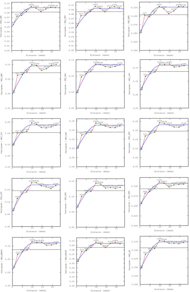
Figure 2 - Empirical (red dotted line) and adjusted (blue line) variogram functions of the residuals from the regression models. The number of pairs at each lag distance, and the standard deviation (black dotted line) are also indicated.
nation. All the months have similar predictors. The lower fits were obtained for mean temperatures in June, July and August (austral winter), with R2
val-ues ranging from 0.924 to 0.930. This is expected because mean values in months with extreme tem-peratures are more difficult to predict than in those with mean or modal values. Considering annual data, the lower fit was obtained for the minimum air tem-perature.
Regression coefficients for altitude always have negative values. As expected, air temperature is negatively correlated to increases of altitude. For latitude, regression coefficients are positive. In this case increases in latitude mean decreases in final temperature values since latitudes in the State of São Paulo were treated as negative values (Southern hemisphere). The equations constructed with each regression coefficient and interception values were used to derive 15 equations predicting the spatial distribution of air temperature by means of map algebra using a Geographic Information Sys-tem.
The spatial structure of the residual values by ordinary kriging was also analyzed. The shapes of the empirical semivariograms show that the residuals present a pattern of spatial dependency (Figure 2). Spherical models to describe the empirical variogram functions of the residuals showed the best goodness of fit according to the minimum weighted least squares criteria.
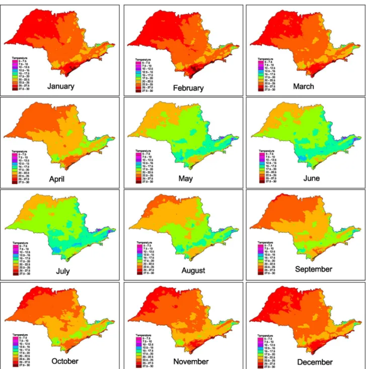
Nuggets range between 0.05-0.1 and variograms stabilize at approximately 100 km. These residual values account for the local variations of tem-perature not adjusted by the regression models. The regression model accuracy can be increased by adding the maps of the kriged residuals (Figure 3) to those obtained with the regression equations. We observe that residuals take the values of ± 0.5ºC in the main part of the State, so that a good fit be-tween the model and the empirical data was obtained. The results for annual temperatures are shown in ures 4 to 6. Monthly temperature results are in Fig-ure 7.
Table 2 shows the mean minimum, mean maximum and mean temperature results for raster layers in monthly and annual basis. The extreme months are June (5.41ºC) and February (28.39ºC). Despite minimum temperatures in May, June and July are lower than 5ºC it has to be noted that mean temperatures are much higher, around 18ºC, considering the whole study area. These low values of temperature are located in high altitude areas in the NE of the coastal moun-tains.
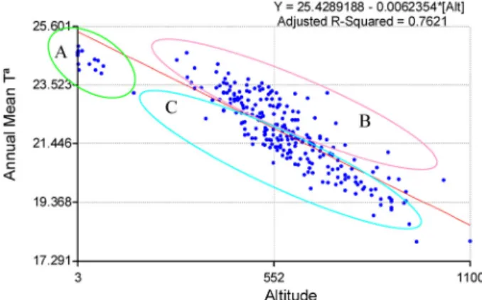
Finally a linear regression analysis to isolate the influence of altitude and latitude on the interpolated val-ues of temperature was made. In Figure 8 the scatterplot of the annual mean temperatures over altitude, and the least square linear regression model are represented. There is a good correlation between altitude and tem-perature (R2 = 0.762). A trend of a decline in tempera-ture with increases in altitude is observed. In this scatterplot three groups of points are distinguished.
Points belonging to area A correspond to data of meteorological stations from the Coastal Re-gion. The oceanic influence in this area causes annual mean temperatures to be lower than the modelled val-ues explained by the simple linear correlation model of altitude over temperature. For similar altitude values, there is a gradient of temperature from points in zone C to those in zone B that can be explained by their latitude position. The cut point between both zones is located at 22.11ºS. Real temperatures in this area tend to be higher than modelled temperatures by this simple regression model. The contrary occurs in zone C. This shows that, in addition to the effect of altitude, there is a certain contribution of latitude to the spatial dis-tribution of temperature.
Plotting annual mean temperatures in relation to latitude (Figure 9) a group of points (zone A) cor-responding again to the same stations of the Coastal Province can be observed. On the other hand, the co-efficient of determination is low, showing a poor weight of latitudes in relation to altitudes when explain-ing the distribution of temperatures. For each latitude Table 2 - Descriptive statistics for the monthly and annual
air temperature layers (451,534 raster cells).
) C º ( n a e m T n a e
M S.D. Min Max
y r a u n a
J 24.51 1.5 10.84 28.10
y r a u r b e
F 24.66 1.5 10.64 28.39
h c r a
M 24.14 1.5 10.16 27.69
l i r p
A 22.06 1.6 8.72 25.17
y a
M 18.75 1.6 5.73 21.58
e n u
J 18.49 1.7 5.41 21.46
y l u
J 18.34 1.7 5.53 21.41
t s u g u
A 20.18 1.9 6.34 23.77
r e b m e t p e
S 21.69 1.9 8.66 5.46
r e b o t c
O 22.75 1.8 9.54 26.17
r e b m e v o
N 23.36 1.7 9.62 26.49
r e b m e c e
D 23.89 1.6 9.89 27.30
n i M l a u n n
A 18.33 1.7 5.31 21.43
x a M l a u n n
A 24.66 1.5 10.64 28.39
n a e M l a u n n
there is a temperature gradient due to the effect of al-titude, the cut point being between zones B and C lo-cated at 570 m.
Therefore, the multiple regression models pro-posed in this study improves the accuracy of simple linear regression models of temperature values over al-titudes.
Altitudes and latitudes for the map raster layers of this study were computed using the GTOPO30 DEM, and the low resolution of this DEM can be a cause of incertitude for the temperature maps. The use of a more accurate DEM of the State would lead to a more realistic distribution of air tem-peratures.
Figure 3 - Maps of the kriged residuals for temperature in the State of São Paulo, Brazil.
Figure 4 - Annual mean minimum temperature in the State of São Paulo, Brazil.
CONCLUSIONS
Multiple regression analysis is a suitable method to model air temperature in the State of São Paulo. The models created can predict air temperature with an ac-curacy greater than 90% in all cases. The spatial dis-tribution of temperature can be explained using only latitude and altitude as independent variables. Longi-tude was, in all analyses, a non-significant variable able to predict air temperatures. The kriging of the residu-als allows to take into account local anomalies into the regression models and thus to improve the final results.
Figure 6 - Annual mean temperature in the State of São Paulo, Brazil.
Linking these regression models to a more accurate DEM would lead to a better spatial pattern of monthly and annual air temperatures in the State of São Paulo.
REFERENCES
BIGG, G.R. Kriging and intraregional rainfall variability in England.
International Journal of Climatology, v.11, p.663-675, 1991.
BURROUGH P.A.; MCDONNELL, R.A. Principles of
Geographical Information Systems. New York: Oxford
University Press, 1998. 333p.
CACHEIRO-POSE, M.; VIEIRA, S.R.; PAZ-GONZÁLEZ, A. Notes for soil conservation history in São Paulo State (Brazil). In: INTERNATIONAL CONGRESS MAN AND SOIL AT THE THIRD MILLENIUM, 3., Valencia, 2002. Proceedings. Logroño: Geoforma Ediciones, 2002.
COLLINS, F.C.; BOLSTAD, P. A comparison of Spatial Interpolation Techniques in Temperature Estimation. In: INTERNATIONAL CONFERENCE / WORKSHOP ON INTEGRATING GIS AND ENVIRONMENTAL MODELING, 3., Santa Fe, 1996.
Proceedings. Santa Fe: NCGIA, 1996. 1 CD-ROM.
DINGMAN, S.L.; SEELY-REYNOLDS, D.M.; REYNOLDS, R.C. Application of kriging to estimating mean annual precipitation in a region of orographic influence. Water Resources Bulletin, v.24, p.329-339, 1988.
FELICÍSIMO-PÉREZ, A.M.; MORÁN-LÓPEZ, R.; SÁNCHEZ-GUZMÁN, J.M.; PÉREZ-MAYO, D. Elaboración del atlas climático de Extremadura mediante un sistema de información geográfica. Geofocus, v.1, p.17-23, 2001.
GOODALE C.L.; ABER, J.D.; OLLINGER, S.V. Mapping monthly precipitation, temperature, and solar radiation for Ireland with polynomial regression and a digital elevation model. Climate Research, v.10, p.51-67, 1998.
GOOVAERTS, P. Geostatistics for natural resources evaluation. New York: Oxford University Press, 1997. 496p. GOOVAERTS, P. Geostatistical approaches for incorporating elevation into the spatial interpolation of rainfall. Journal of Hydrology, v.228, p.113-129, 2000.
GTOPO30: “Global 30 Arc Second Elevation Data Set”. Reston: US Geological Survey, 1996. Available at: http://edcwww.cr.usgs.gov/ landdaac/gtopo30/gtopo30.html. Accessed on: 12 nov. 2004. HUTCHINSON, M.F. Climatic analyses in data sparse regions. In:
CHOW, M.C.; BELLAMY, J.A. (Ed.). Climatic risk in crop production. Models and management for the semiarid tropics and subtropics. Wallingford: CAB International, 1991. p.55-71. LENNON, J.J.; TURNER, J.R.G. Predicting the spatial distribution of climate temperature in Great Britain. Journal of Animal Ecology, v.64, p.370-392, 1995.
MARQUINEZ, J.; LASTRA, J.; GARCIA, P. Estimation models for precipitation in mountainous regions: The use of GIS and multivariate analysis. Journal of hydrology, v.270, p.1-11, 2003.
NINYEROLA, M. Modelització climática mitjançant tècniques SIG i la seva aplicació a l’anàlisi quantitativa de la distribució d’espècies vegetals a l’Espanya peninsular. Barcelona: Universitat Autónoma de Barcelona, 2000. 202p. (Thesis - Ph.D.).
NINYEROLA, M.; PONS, X.; ROURE, J.M. A methodological approach of climatological modelling of air temperature and precipitation through GIS techniques. International Journal of Climatology, v.20, p.1823-1841, 2000.
PHILIPS, D.L.; DOLPHY, J.; MARKS, D. A comparison of geostatistical procedures for spatial analysis of precipitation in mountainous terrain. Agricultural and Forest Meteorology, v.58, p.119-141, 1992.
SAVELIEV, A.A.; MUCHARAMOVA, S.S.; PILIUGIN, G.A. Modeling of the daily rainfall values using surfaces under tension and kriging. Journal of Geographic Information and Decision Analysis, v.2, p.58-71, 1998.
SILVA, A.L.; ROVERATTI, R.; REICHARDT, K.; BACCHI, O. O.S.; TIMM, L.C.; OLIVEIRA, J.C.M.; DOURADO NETO, D. Variability of water balance components in a coffee crop grown in Brazil. Scientia Agricola, v. 63, p.105-114, 2006. VALERIANO, M.M.; PICINI, A.G. Uso de sistema de informação
geográfica para a geração de mapas de medias mensais de temperatura do Estado de São Paulo. Revista Brasileira de Agrometeorologia, v.8, p.255-262, 2000.
WORLD METEOROLOGICAL ORGANIZATION. A note on climatological normals. Geneva: WMO, 1967. (Technical Note, 208).
WOTLING, G.; BOUVIER, C.H.; DANLOUX, J.; FRITSCH, J.-M. Regionalization of extreme precipitation distribution using the principal components of the topographical environment.
Journal of Hydrology, v.233, p.86-101, 2000.
Received May 30, 2006 Accepted June 22, 2007
Figure 8 - Scatterplot of annual mean temperature over altitude.