Scientiic/Technical Article
http://dx.doi.org/10.1590/2318-0331.0217170068
Eficient number of calibrated cross sections bottom levels on a hydrodynamic model
using the SCE-UA algorithm. Case study: Madeira River
Número eficiente de cotas de fundo de seções transversais calibráveis em um modelo hidrodinâmico usando o algoritmo SCE-UA. Estudo de caso: Rio Madeira
João Paulo Lyra Fialho Brêda1, Juan Martín Bravo1 and Rodrigo Cauduro Dias de Paiva1
1Universidade Federal do Rio Grande do Sul, Porto Alegre, RS, Brazil
E-mails: [email protected] (JPLFB), [email protected] (JMB), [email protected] (RCDP)
Received: May 03, 2017 - Revised: July 14, 2017 - Accepted: August 20, 2017
ABSTRACT
Hydrodynamic models are important tools for simulating river water level and low. A considerable fraction of the hydrodynamic model errors are related to parameters uncertainties. As cross sections bottom levels considerably affect water level simulation, this parameter has to be well estimated for lood studies. Automatic calibration performance and processing time depend on the search space dimension, which is related to the number of calibrated parameters. This paper shows the application of the Shufled Complex Evolution (SCE-UA) optimization algorithm to assess the number of cross sections bottom levels used in calibration. Also was evaluated the extent of algorithm exploration regarding computational processing time and accuracy. It was tested the calibration of 2, 4, 7 and 10 cross sections bottom levels (2PAR, 4PAR, 7PAR and 10PAR calibration conigurations) of a 1,100 km reach of the Madeira River. 7PAR and 10PAR representation had better itness (lower objective function value) on cross sections used for calibration; however, the error on other cross sections (2 validation gauging stations) was higher than 2PAR and 4PAR calibration. The short number (5) of gauging stations used in calibration has limited the number of calibrated parameters to represent adequately the river level proile. Finally, this paper shows a contribution for the parsimonious selection of parameters regarding the spatial distribution of observation sites used in calibration.
Keywords: Bottom levels; Calibration; SCE-UA; Parameters; Parsimony; Hydrodynamic models.
RESUMO
Modelos hidrodinâmicos são ferramentas importantes para simular nível e vazão de rio. Uma fração considerável dos erros do modelo hidrodinâmico está relacionada com as incertezas dos parâmetros. Como a cota do fundo nas seções transversais afetam signiicativamente a simulação do nível d’água, esse parâmetro deve ser bem estimado para estudos de inundação. O desempenho da calibração automática e seu tempo de processamento dependem da dimensão do espaço de busca, que está relacionada com o número de parâmetros calibráveis. Este artigo utiliza o algoritmo de otimização Shufled Complex Evolution (SCE-UA) para avaliar o número de cotas de fundo de rio calibráveis e o nível de exploração do algoritmo observando o tempo de processamento computacional e a precisão do método. Foram testadas calibrações de 2, 4, 7 e 10 cotas de fundo de seções transversais (conigurações de calibração 2PAR, 4PAR, 7PAR e 10PAR) em um trecho de 1.100 km do Rio Madeira. 7PAR e 10PAR apresentaram melhor aptidão (menor valor de função-objetivo) em seções usadas na calibração; no entanto, o erro em diferentes seções (2 estações luviométricas de validação) foi maior do que as conigurações 2PAR e 4PAR. O pequeno número (5) de estações luviométricas utilizadas na calibração limitou o número de parâmetros calibráveis para representar adequadamente o peril longitudinal de nível do rio. Por im, este trabalho contribuiu para a seleção parcimoniosa de parâmetros calibráveis observando à distribuição espacial das observações utilizadas na calibração.
INTRODUCTION
Hydrodynamic models are important tools for understanding river dynamics (PAIVA et al., 2013; PONTES et al., 2015); discharge, water level and lood forecasting (FAN et al., 2014a) and simulating pollutant dispersion (CAVALCANTE; MENDES, 2014). For large rivers, these models are often based on one-dimensional momentum and mass conservation equations, named as the Saint Venant equations. Saint Venant full resolution (PAIVA et al., 2013) and some simpliied models, such as the 1D Inertial model (YAMAZAKI; ALMEIDA; BATES, 2013; FAN et al., 2014b), can successfully account river water level and adequately represent backwater effects, storage volume and river-loodplain water exchanges on river basin.
The hydrodynamic model performances are considerably dependent to the chosen set of parameters values. Cross section wetted area, given by its width and depth, bottom slope and channel roughness control the modeled low state variables. For a large-scale basin, data from remote sensing can be helpful for parameter estimation, as ield measurements are insuficient to embrace the whole river. Aerial images can facilitate deining river width (PAVELSKY; SMITH, 2008), and Digital Elevation Models (DEM) contributes identifying the drainage system (SIQUEIRA et al., 2016a). On the other hand, parameters such as the river bottom level carry out higher uncertainty as no remote sensing techniques for deep rivers are available other than local measurements (p.e. using ADCP). Therefore, the hydrodynamic model usually is submitted to a calibration process, which is a parameter adjustment to improve model itness to observation data.
Although most of model applications focus on river roughness coeficient calibration – since it is a subjective coeficient that simpliies forces related to head losses – Paiva et al. (2013) had shown that errors in river bottom level could affect signiicantly simulations of water surface elevation, lood wave travel time and loodplain area extent. In addition, Wood et al. (2016) calibrated the LISFLOOD-FP model using SAR (synthetic aperture radar) images and observed that simulated lood extent is more sensible to variation on bathymetry than roughness coeficient. Indeed, in large rivers, cross section information (e.g. bottom levels) is sparse or missing and then could be incorporated to the calibration process as a set of parameters.
The calibration process can be manual or automatic. Manual calibration depends on the model user expertise, which selects the next set of parameters values based on the previous results mainly by visual analysis (BOYLE; GUPTA; SOROOSHIAN, 2000). As a negative point manual calibration can be exhaustive and time-consuming, especially in high-complexity models, and still could not reach true optima parameter values. On the other hand, automatic calibration algorithms evaluate model results through a mathematical criteria and search for better itted parameters sets by optimization methods, hence eliminating subjectivity.
Automatic calibration algorithms can either be of local search or global search. Local search techniques are designed to ind local optimum thus becomes deeply dependent of the startup parameters sets. Global search techniques commonly use a probabilistic approach in order to improve exploration over the search space, consequently increasing their chances to ind the
global optimum instead of converging to the closest optimum (region of attraction) as local search techniques (DUAN, 2003).
In 1992, Duan, Sorooshian and Gupta presented the Shufled Complex Evolution – University of Arizona algorithm (SCE-UA) which was proved to be a robust global search calibration method. This algorithm was introduced in a CRR (Conceptual Rainfall-Runoff) model calibration context, being initially tested for a six-parameters model (DUAN; SOROOSHIAN; GUPTA, 1992). Subsequent SCE-UA applications had kept a small number of model parameters to be calibrated, for example: six in Siqueira et al. (2016b), eleven in Blasone, Madsen and Rosbjerg (2007), two to thirteen in Duan, Sorooshian and Gupta (1994), sixteen in Zhang et al. (2009) and eighteen in Eckhardt and Arnold (2001).
However, the number of parameters used to represent a hydrological system can be much higher than a couple of dozens, especially due to the growing complexity of current models. High number of parameters increases the search space dimension and consequently the quantity of model simulations needed in the calibration process. Thus complex models calibration demands longer computational processing time, which might be unfeasible. Eventually calibration accuracy becomes limited by computational capacity.
To bypass this situation, correlated parameters can be adjusted in a ixed ratio in order to reduce the search space dimension (ECKHARDT; ARNOLD, 2001; BLASONE; MADSEN; ROSBJERG, 2007). Decreasing number of parameters might also help lowering costs since less ield measurements for parameters estimation would be required.
Previous researches have evaluated the impact of the number of calibrated parameters on the model accuracy of distributed, lumped or statistical hydrological models (HER; CHAUBEY, 2015; SCHOUPS; VAN DE GIESEN; SAVENIJE, 2008). However it is necessary to relate these factors to computational time demand and extend the subject to include hydraulic models likewise.
For this purpose, the present paper evaluates calibration effectiveness by investigating how many cross sections bottom levels should be calibrated on a 1D hydraulic model aiming to balance between processing time and model accuracy. The studied area comprises an 1,100 km reach of the Madeira River, in the Amazon River basin, where four optimization conigurations with different numbers of calibrated cross sections bottom level (2, 4, 7 and 10) were assessed.
METHODOLOGY Hydrodynamic modeling
lat
A Q q
t x
∂ +∂ =
∂ ∂ (1)
/
2
4 3 g Q Q n
Q gA y 0
t x AR
∂ + ∂ + =
∂ ∂ (2)
Where Q is the discharge; A is the cross section area; qlat is lateral inlow by unit of length; g is gravity; y is the water surface level (given by depth + bottom level, which is the calibrated parameter); n is Manning roughness; R is the hydraulic radius; x and t are the
independent variables that represent longitudinal distance and time, respectively.
The numerical approach to solve the 1D inertial model equation system is described by Fan et al. (2014b). It is an explicit scheme that calculates low from the momentum equation and water level/depth from the continuity equation and uses an adaptive time step based on the Courant-Friedrichs-Levy condition. The modeled cross section is rectangular (wetted area = depth × width) and the water volume that overlows riverbanks behaves as water storage.
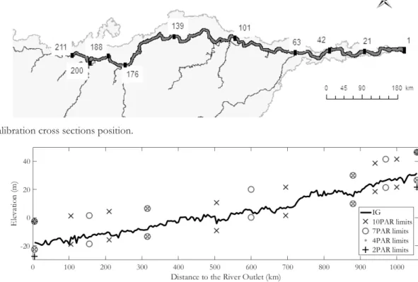
The case study was an 1,100 km reach of the Madeira river, starting at the city of Porto Velho and ending at the river’s outlet on the Amazon River (Figure 1). The Madeira River basin drainage area is about 1.4 million km2, which accounts for 20%
of the Amazon basin. The portion of the basin upstream of the modeled river reach corresponds to ¾ of the total drainage area. This river reach was selected for this case study because it has no signiicant hydraulic structures or point lateral inlows that would require complex modelling.
The modeled river reach was discretized in 211 reaches of approximately 5 km length. Each reach width was determined using a river mask obtained from near infrared images (band 5) of Landsat 8. The adopted Manning roughness coeficient was 0.030. As boundary conditions, it was used a water level time series at the outlet reach and a low time series at the irst reach upstream, both data obtained from Brazilian National Water Agency (ANA) gauging station – 15940000 and 15400000, respectively.
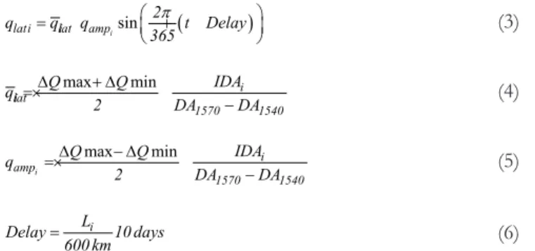
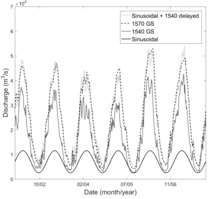
A simpliied method was used to estimate lateral inlow through a sinusoidal function proportional to the incremental drainage area of the respective reach, obtained by an approximation of the difference between two ANA low gauging stations distant 600 km from each other (15400000 and 15700000 – Figure 1). The lateral inlow (qlati) was calculated by the following equations
and results are presented in Figure 2:
( )
sin
i
lati liat amp 2
q q q t Delay
365π
= + −
(3)
max min
i
liat
1570 1540
IDA
Q Q
q
2 DA DA
∆ + ∆
=× − (4)
max min
i
i
amp
1570 1540
IDA
Q Q
q
2 DA DA
∆ − ∆ =×
− (5)
i
L
Delay 10 days 600 km
= (6)
Where t is the simulation time; ∆Qmax and ∆Qmin is the maximum and minimum discharge difference between the two gauging stations (15400000 and 15700000), IDAi is the reach i incremental drainage area; DA is the accumulated drainage area of the gauging stations; Li is the distance between the river reach and the gauge station 15400000; and 10 days relates to the delay in which the two gauging stations discharge series present the highest correlation.
SCE-UA
The SCE-UA (DUAN; SOROOSHIAN; GUPTA, 1992) algorithm is a global search technique that combines the concepts of controlled random search, complex shufling and competitive evolution to minimize an objective-function (OF). This algorithm is able to overcome the main calibration problems such as: multiple regions of attraction, roughness surface due to discontinuous derivatives, parameter interdependency and varying sensitivity
(DUAN; SOROOSHIAN; GUPTA, 1994). A summary of this method is given on the following paragraphs.
Firstly, a population of s points (set of parameters values) is randomly generated. Each point is evaluated by an OF which typically is related to the difference between the model results and the observed values. Then the population is ranked based on the OF values and divided into p complexes of m points. Each complex evolves alone within a generation, according to a Competitive Complex Evolution (CCE) procedure. After a generation, the complexes are grouped and shufled to form new complexes in the next generation. This process continues until a convergence criterion is attached or after a pre-deined number of generations.
The CCE procedure is based on the Simplex optimization method (NELDER; MEAD, 1965). Initially q points from the complex are selected to form a subcomplex. The selection considers a trapezoidal probability distribution in which the most adapted points (lower OF values) have higher chances to be selected. Then a
procedure similar to Simplex takes place. Firstly the algorithm calculates the centroid of the subcomplex points except the less adapted one (higher OF value), then new points are evaluated through a relection step, a contraction step or a mutation step. This process is repeated β times followed by a complex shufled for the next generation (Figure 3). For a detailed explanation of the SCE-UA algorithm the reader is kindly redirected to Duan, Sorooshian and Gupta (1992).
For the purpose of this paper most of the parameters of the SCE-UA algorithm was set to default values as in Duan, Sorooshian and Gupta (1994): m = 2n + 1, q = n + 1 and β = 2n + 1, where n is the number of model parameters to be calibrated. Only the number of complexes (p = 2, 4 or 6), which is an important parameter related to the exploration of the search space, was previously tested to assess the algorithm convergence. It was considered that the calibration process reaches the convergence criteria when the relative difference between the population median and lower OF values is less than 0.5%.
Figure 2. Lateral inlow method demonstration.
Experiment design
The SCE-UA algorithm was applied to calibrate the bottom level of the cross sections of the hydrodynamic model. Four different conigurations were tested during calibration of the cross section bottom levels:
a) 2 parameters (2PAR) - only the irst and the last cross sections bottom level are calibrated (cross sections 1 and 211, Figure 4);
b) 4 parameters (4PAR) - the irst, the last and two other reaches where most important tributaries join the main river (cross sections 1, 63, 176 and 211, Figure 4) had their bottom level calibrated;
c) 7 parameters (7PAR) - the four previous ones and one reach between each of them (cross sections 1, 31, 63, 120, 176, 194 and 211, Figure 4) had their bottom level calibrated; d) 10 parameters (10PAR) - the four cross sections presented
in b) and other two equally-spaced reaches between them (cross sections 1, 21, 42, 63, 101, 139, 176, 188, 200 and 211 – Figure 4) had their bottom level calibrated. The bottom levels of the remaining internal reaches were deined through linear interpolation of the closest cross sections selected for calibration. SCE-UA was tested 10 times for each value of p (2, 4 and 6) in order to verify the algorithm performance.
To compare results and to deine the search space, an initial guess (IG) of the river bottom level was acquired reducing a maximum depth from the river surface level obtained from a 500 m resolution digital elevation model (DEM) of the Shuttle Radar Topography Mission (SRTM – FARR et al., 2007). The maximum depth was estimated by a geomorphologic equation, presented
on Paiva et al. (2013), which assumes the maximum depth (h) as a function of the drainage area (DA):
( )
(
( )
)
.. 2 0 20
h m =1 25 DA km× (7)
The search space was deined as 15 m above and 5 m bellow of the bottom levels initial guess (except for 2 parameters coniguration, which was 15 m above and 10 m below). The search space limits is shown on the Figure 5.
The objective function of the calibration process was the root mean squared error (RMSE) based on data from ive water level gauging stations from ANA – 15400000, 15630000, 15700000, 15850000 and 15900000 (Figure 1). Every water level gauging station used in this paper was georeferenced to EGM08 geoid according to Moreira (2016). Data from these gauging stations were compared to the model results at the closest cross section, which were 211, 163, 91, 63 and 34 respectively.
The calibration process refers to a three years simulation period with 2 warm up months (Jan and Feb of 2002) and the remaining time was used for RMSE calculation (Mar/2002 to Dec/2004). Data from Jan/2005 to Jun/2010 were used to validate the results obtained from calibration (temporal validation). Additionally two other water level gauging stations (15490000 and 15860000) were used in order to ind out if the model represents other reaches of the river satisfactorily (spatial validation). The gauging stations water level time series are presented on box plots at Figure 6.
RESULTS AND DISCUSSION
First, it was assessed whether the selected coniguration of the SCE-UA algorithm was able to ind the global optimum set of parameters values. For this purpose the SCE-UA algorithm
Figure 4. Calibration cross sections position.
was tested using different number of complexes (p = 2, 4, 6) and four parameter conigurations (n = 2, 4, 7 and 10). Each test was repeated 10 times to verify the performance.
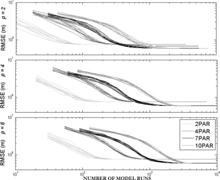
The Figure 7 exhibits the algorithm performance relating the number of hydrodynamic model runs and the SCE-UA population itness represented by the median of the OF values. It can be observed that as the number of calibration parameters increases, more hydrodynamic model runs were necessary for algorithm convergence. The calibration of 10 parameters (10PAR) needed approximately 2, 5 and 15 times more hydrodynamic model runs to converge when compared to the calibration of 7 (7PAR), 4 (4PAR) and 2 (2PAR) parameters, respectively. Regarding the number of complexes used for the SCE-UA algorithm coniguration, it seems that the quantity of hydrodynamic model runs needed for convergence increases by a nearly constant value. For instance, when 4 parameters are calibrated the number of hydrodynamic model runs necessary for convergence was increased in approximately 300 for every 2 adding complexes, while in a 10PAR coniguration this constant value is around 1000.
About effective computational demand, the tests were performed on an 8 GB RAM Intel Core i5 CPU; each model simulation takes about 4 seconds. Thus, while a 2PAR-two-complexes calibration coniguration takes about 7 minutes to converge (100 model runs), a 10PAR-six-complexes takes approximately 4.5 hours (4000 model runs).
Table 1 demonstrates the highest and lowest OF values from 10 calibration processes of each coniguration. As observed, the OF (RMSE) value decreases as the number of parameters increases. However, only a slight difference in the OF value was observed between the calibration of 2 and 4 parameters, although the 4 parameters calibration needs 3 times more hydrodynamic model runs to converge (similar results when compared 10PAR and 7PAR). On the other hand, the 10PAR and 7PAR coniguration calibration resulted in a 20% lower OF value compared to the 2PAR and 4PAR. Thus, increasing the parameters number can lead to either a slight or a high reduction of the OF value, although it consistently raises the number of hydrodynamic model runs. These facts enhance the discussion of which should be the number of calibration parameters since a signiicant increase on
Figure 7. Number of Model Runs necessary for convergence related to number of complexes (p) and the number of calibrated parameters.
processing time does not guarantee a considerable improvement on model itness.
Table 1 also informs the algorithm precision rate, which was deined as the number of times the calibration procedure reached the exact same parameters values as the best calibration parameters set (lowest OF). The 2PAR and 4PAR coniguration calibration achieved the same parameters values in all calibration processes, which probably means that the OF surface roughness is low and it has only a main region of attraction. In contrast, the 10PAR calibration has not repeated a single set of parameters. Although the precision result looks disappointing at irst sight, there is not much difference between the 10PAR calibration outcomes. The highest and lowest OF values differ only in 0.1%. That happens because the bottom levels of the downstream reaches do not seem to inluence signiicantly the OF value (Figure 8) since there is a boundary condition that controls water elevation at the river mouth, creating a highly rough surface near the global optimum. Regarding to the 7PAR coniguration, it can be seen that there is a second region of attraction (Table 1) which accounts for a local optimum with OF value of 0.6815 m; however setting the number of complexes to 4 basically ensures enough exploration to ind the global optimum.
As has been noted, the number of complexes selected has made a slight impact on the results of the calibration. However, raising
the number of complexes increased signiicantly the number of model simulations necessary for convergence. 2PAR and 4PAR coniguration calibration had always converged to the same set of parameters and the 10PAR calibration had reached almost the same OF value. Although a higher number of complexes contributed inding the global optimum of the 7PAR coniguration, the local optimum OF value (0.6815 m) reached in 2 of 10 times, was still better than the value obtained with a lower number of parameters. Thus, it becomes questionable whether is necessary to raise exploration by increasing the number of complexes and consequently the chances of inding global optimum or just search for an acceptable local optimum and save computational processing time. In this study case, it seems suficient to use two complexes for any calibration coniguration aiming to reduce computational cost.
The calibrated bottom levels obtained in the four different conigurations are presented in Figure 9. It can be observed that all conigurations have converged to similar values of bottom levels at the “middle region”, limited between 300 and 850 km from the river outlet. It probably means the bottom levels at the middle region that provide the most accurate water level simulation is somewhere near to the calibrated values. Since 10PAR and 7PAR have more degrees of freedom, especially at the extremities of the reach, some “bumps” were created on the inal bottom level to improve level estimations at the gauging stations cross sections. 10PAR calibration has built a small barrier upstream followed by a steep region, creating an unreal but effective bottom level (Figure 9).
As example of the results, observed and simulated surface water levels from August 2007 to December 2008 in each gauging station are presented in Figure 10. The difference between simulated and observed water levels is about few meters during the high and low seasons. The calibration process has virtually eliminated
Table 1. OF RMSE values and Precision Rate.
OF – RMSE (m) Precision Rate Higher Lower p = 2 p = 4 p = 6
2PAR 0.7591 0.7591 10/10 10/10 10/10
4PAR 0.7572 0.7572 10/10 10/10 10/10
7PAR 0.6815 0.6009 08/10 10/10 10/10
10PAR 0.5855 0.5850 01/10 00/10 00/10
Figure 8. Calibrated bottom levels of 10PAR the coniguration.
the model bias. However, the simulated levels amplitude is clearly overestimated. That is due to other parameters uncertainties such as Manning roughness or cross section width, which could be calibrated as well. Thus, the irregular bottom level obtained from the 10PAR calibration might be an attempt to reduce the simulated level amplitude at the gauging stations.
High values of RMSE from the initial guess bottom (IG) level simulation shows that calibration is essential for acquiring reasonable results as observed in validation outcomes (Table 2). Even a simple calibration coniguration (2PAR) can signiicantly improve simulations of the water level when parameters uncertainties are considerable. Most RMSE values of calibrated models were below 1 m. On the other hand, the IG RMSE was higher, reaching 9 m on gauging stations 15400000 and 15630000, which signiicantly affects quantifying river-loodplain water exchanges.
Validation results were similar to calibration results at the gauging stations used as observation sites on the calibration process (light grey area of Table 2). The RMSE values have remained low
and the calibration processes with more parameters have presented better results. 10PAR mean RMSE was 0.2 m lower than 2PAR and 4PAR, which represents a 25% error reduction (Table 2). Therefore, the temporal validation has shown that increasing the number of calibration parameters improves the model accuracy related to the gauging stations used on the calibration process.
The situation described above inverts if it is also considered the gauging stations 15860000 and 15490000, which were not used during the calibration process (dark grey on Table 2), on the mean RMSE calculation (spatial validation). A parsimonious representation of the bottom levels revealed better performance on both gauging stations. 2PAR and 4PAR calibrations have maintained almost the same RMSE values (which are around 1 m) while 7PAR and 10PAR have doubled or triplicated the RMSE values compared to other gauging stations (Table 2). Although the gauging stations 15490000 and 15400000 are relatively close (Figure 1), around 75 km distance, there are considerable differences between the RMSE values. These results conirm that the irregular bottom levels created by the 7PAR and 10PAR calibration on the river reach extremities deviate from the real bottom level. Therefore, if the model purpose is to simulate the river level proile or obtain water level series on speciic points apart from gauging stations used in calibration, then the 4PAR or 2PAR calibration conigurations (more parsimonious) are indicated.
CONCLUSION
This paper has focused on evaluating computational demand and accuracy of the calibration processes with different number of parameters (2, 4, 7 and 10). It is presented a case in which it is possible to discuss the main problems related to calibration
Table 2. Validation results (RMSE) (dark grey - only validation GS; light grey - calibraion/validation GS).
Gauging Station IG 2PAR 4PAR 7PAR 10PAR
15400000 9.017 1.183 1.068 0.611 0.529
15630000 9.130 0.806 0.884 0.871 0.809
15700000 6.111 1.009 0.941 0.847 0.833
15850000 3.300 0.692 0.726 0.661 0.640
15900000 1.607 0.781 0.814 0.656 0.581
Partial Mean 5.833 0.894 0.887 0.729 0.678
15860000 2.662 0.885 0.885 1.125 1.479
15490000 9.886 1.034 1.105 3.163 3.878
Total Mean RMSE 5.959 0.913 0.918 1.134 1.250
parameters selection, including overitting and observation sites spatial distribution. In addition, this study highlights the importance of calibrating river bottom level for water elevation studies. The case study was an 1100 km reach of the Madeira River simulated by a hydrodynamic model. The conigurations with 2 and 4 parameters have presented results that are more consistent and less time demanding.
The quantity of cross sections that should be selected for a hydraulic model calibration process is highly dependent of the observation spatial distribution. If there are only a few observation sites, the calibrated cross sections will not represent well the whole river. Indeed the calibration will adjust the parameters to provide the best itness to the calibration gauging stations and neglect the real river level proile. In such cases, less calibrated parameters results in a more realistic river proile estimation. However if the model purpose is matching simulated to observation water levels in gauging stations, then calibration with more parameters can provide better results.
One way that could reduce level proile representation problem is forcing downstream bottom level to be lower than upstream. This is a parameter limitation that can avoid imaginary bottom levels as in the 10PAR calibration. Another option is to create a correlated bottom level as in Yoon et al. (2012), thus close cross sections bottom levels will not differ considerably.
Concerning this case study, the OF value at the local optima was very close to the OF value at the global optima. Thus reducing the calibration algorithm exploration becomes an option to decrease the number of simulations necessary for algorithm convergence and consequently reduce the computational demand. After all it is user task to balance between accuracy and processing time, and to be careful with overitting and parsimony.
Although the bottom elevation accounts for the main errors in surface water level, alternative parameters could also be tested. Since the calibrated model simulations presented higher amplitude than observed levels, probably the remaining improvements in model itness is related to calibration of other parameters such as Manning roughness or cross section width. Therefore, a mixed Manning roughness and bottom level calibration turn out to be a promising choice for achieving better outcomes.
These results enhance the knowledge about calibration settings. Her and Chaubey (2015) revealed that raising the number of calibration parameters on the hydrological model SWAT diminish parameters uncertainty and improve model accuracy, however the authors only tested few observation sites and did not consider parameters spatial distribution. On the other hand, the present study has shown that, regarding river cross sections on hydraulic models, a parsimonious number of parameters can provide more reliable results.
This study introduces the importance of selecting a suficient number of cross sections to adequately represent the river channel on a hydraulic model. Nonetheless this paper presents only a case study. It is recommended that future researches evaluate rivers with different sizes and shapes to test if the cited conclusions apply to other situations.
In conclusion, this paper has presented contributions regarding parsimonious choices of calibration parameters, specially related to river bottom level. Fewer parameters might not only save processing
time but also improves model performance. It is commonly assumed that the model would adjust better as the number of calibrated parameters increases; however, this quantity should rely on the number of observation sites and the parameters spatial correlation.
REFERENCES
BATES, P. D.; HORRITT, M. S.; FEWTRELL, T. J. A simple inertial formulation of the shallow water equations for efficient two-dimensional flood inundation modelling. Journal of Hydrology, v. 387, n. 1-2, p. 33-45, 2010. http://dx.doi.org/10.1016/j. jhydrol.2010.03.027.
BLASONE, R.-S.; MADSEN, H.; ROSBJERG, D. Parameter estimation in distributed hydrological modelling: comparison of global and local optimization techniques. Hydrology Research, v. 38, n. 4-5, p. 451-476, 2007. http://dx.doi.org/10.2166/nh.2007.024.
BOYLE, D. P.; GUPTA, H. V.; SOROOSHIAN, S. Toward improved calibration of hydrologic models: combining the strengths of manual and automatic methods. Water Resources Research, v. 36, n. 12, p. 3663-3674, 2000. http://dx.doi.org/10.1029/2000WR900207.
CAVALCANTE, R. B. L.; MENDES, C. A. B. Calibração e validação do módulo de correntologia do modelo IPH-A para a Laguna dos Patos (RS / Brasil). Revista Brasileira de Recursos Hídricos, v. 19, n. 3, p. 191-204, 2014. http://dx.doi.org/10.21168/rbrh. v19n3.p191-204.
DUAN, Q. Global optimization for watershed model calibration. In: DUAN, Q.; GUPTA, H. V.; SOROOSHIAN, S.; ROUSSEAU, A. N.; TURCOTTE, R. (Orgs.). Calibration of watershed models. Washington: American Geophysical Union, 2003. cap. 6.
DUAN, Q.; SOROOSHIAN, S.; GUPTA, V. Effective and efficient global optimization for conceptual rainfall-runoff models. Water Resources Research, v. 28, n. 4, p. 1015-1031, 1992. http://dx.doi. org/10.1029/91WR02985.
DUAN, Q.; SOROOSHIAN, S.; GUPTA, V. K. Optimal use of the SCE-UA global optimization method for calibrating watershed models. Journal of Hydrology, v. 158, n. 3, p. 265-284, 1994. http:// dx.doi.org/10.1016/0022-1694(94)90057-4.
ECKHARDT, K.; ARNOLD, J. Automatic calibration of a distributed catchment model. Journal of Hydrology, v. 251, n. 1, p. 103-109, 2001. http://dx.doi.org/10.1016/S0022-1694(01)00429-2.
FAN, F. M.; COLLISCHONN, W.; MELLER, A.; BOTELHO, L. C. Ensemble streamflow forecasting experiments in a tropical basin: The São Francisco river case study. Journal of Hydrology, v. 519, p. 2906-2919, 2014a. http://dx.doi.org/10.1016/j.jhydrol.2014.04.038.
FARR, T. G.; ROSEN, P. A.; CARO, E.; CRIPPEN, R.; DUREN, R.; HENSLEY, S.; KOBRICK, M.; PALLER, M.; RODRIGUEZ, E.; ROTH, L.; SEAL, D.; SHAFFER, S.; SHIMADA, J.; UMLAND, J.; WERNER, M.; OSKIN, M.; BURBANK, D.; ALSDORF, D. The shuttle radar topography mission. Reviews of Geophysics, v. 45, 2007.
HER, Y.; CHAUBEY, I. Impact of the numbers of observations and calibration parameters on equifinality, model performance, and output and parameter uncertainty. Hydrological Processes, v. 29, n. 19, p. 4220-4237, 2015. http://dx.doi.org/10.1002/hyp.10487.
MOREIRA, D. M. Geodésia aplicada ao monitoramento hidrológico da bacia amazônica. 2016. 254 f. Tese (Doutorado em Engenharia Civil) - Programa de Pós-graduação em Engenharia Civil, Universidade Federal do Rio de Janeiro, Rio de Janeiro, 2016.
NELDER, J. A.; MEAD, R. A simplex method for function minimization. The Computer Journal, v. 7, n. 4, p. 308-313, 1965. http://dx.doi.org/10.1093/comjnl/7.4.308.
PAIVA, R. C. PAIVA, R. C. D.; BUARQUE, D. C.; COLLISCHONN, W.; BONNET, M.-P.; FRAPPART, F.; CALMANT, S.; BULHÕES MENDES, C. A. Large-scale hydrologic and hydrodynamic modeling of the Amazon River basin. Water Resources Research, v. 49, n. 3, p. 1-18, 2013. http://dx.doi.org/10.1002/wrcr.20067.
PAVELSKY, T. M.; SMITH, L. C. RivWidth: a software toll for the calculation of river widths from remotely sensed imagery. IEEE Geoscience and Remote Sensing Letters, v. 5, n. 1, p. 70-73, 2008. http://dx.doi.org/10.1109/LGRS.2007.908305.
PONTES, P. R.; COLLISCHONN, W.; FAN, F. M.; PAIVA, R. C.; BUARQUE, D. C. Modelagem hidrológica e hidráulica de grande escala com propagação inercial de vazões. Revista Brasileira de Recursos Hídricos, v. 20, n. 4, p. 888-904, 2015. http://dx.doi. org/10.21168/rbrh.v20n4.p888-904.
SCHOUPS, G.; VAN DE GIESEN, N. C.; SAVENIJE, H. H. G. Model complexity control for hydrologic prediction. Water Resources Research, v. 44, 2008.
SIQUEIRA, V. A.; FLEISCHMANN, A. S.; JARDIM, P. F.; FAN, F. M.; COLLISCHONN, W. IPH-Hydro tools: uma ferramenta open source para determinação de informações topológicas em bacias hidrográficas integrada a um ambiente SIG. Revista Brasileira de Recursos Hídricos, v. 21, n. 1, p. 274-287, 2016a.
SIQUEIRA, V. A.; SORRIBAS, M. V.; BRAVO, J. M.; COLLISCHONN, W.; LISBOA, A. M. V.; TRINIDAD, G. G. V. Real-time updating of HEC-RAS model for streamflow forecasting using an optimization algorithm. Revista Brasileira de Recursos Hídricos, v. 21, n. 4, p. 855-870, 2016b. http://dx.doi.org/10.1590/2318-0331.011616086.
WOOD, M.; HOSTACHE, R.; NEAL, J.; WAGENER, T.; GIUSTARINI, L.; CHINI, M.; CORATO, G.; MATGEN, P.; BATES, P. Calibration of channel depth and friction parameters in the LISFLOOD-FP hydraulic model using medium-resolution SAR data and identifiability techniques. Hydrology and Earth System Sciences, v. 20, n. 12, p. 4983-4997, 2016. http://dx.doi.org/10.5194/ hess-20-4983-2016.
YAMAZAKI, D.; ALMEIDA, G. A. M. D.; BATES, P. D. Improving computational efficiency in global river models by implementing the local inertial flow equation and a vector-base driver network map. Water Resources Research, v. 49, n. 11, p. 7221-7235, 2013. http://dx.doi.org/10.1002/wrcr.20552.
YOON, Y.; DURAND, M.; MERRY, C. J.; CLARK, E. A.; ANDREADIS, K. M.; ALSDORF, D. E. Estimating river bathymetry from data assimilation of synthetic SWOT measurements. Journal of Hydrology, v. 464-465, p. 363-375, 2012. http://dx.doi. org/10.1016/j.jhydrol.2012.07.028.
ZHANG, X.; SRINIVASAN, R.; ZHAO, K.; LIEW, M. V. Evaluation of global optimization algorithms for parameter calibration of a computationally intensive hydrologic model. Hydrological Processes, v. 23, n. 3, p. 430-441, 2009. http://dx.doi.org/10.1002/hyp.7152.
Authors contributions
João Paulo Lyra Fialho Brêda: work idealization, development of the hydrodynamic model, coupling model with the global optimization algorithm, acquisition of validation data, generation and exposure of results; text writing.
Juan Martín Bravo: work idealization, writing of the sce-ua global optimization code, guidance on the coniguration of the optimization algorithm, text revision.