Paulo Cesar Plaisant Junior EMBRAER São José dos Campos/SP – Brazil
Flávio Luiz de Silva Bussamra* Instituto Tecnológico de Aeronáutica São José dos Campos/SP – Brazil [email protected]
Francisco Kioshi Arakaki EMBRAER São José dos Campos/SP – Brazil [email protected]
*author for correspondence
Finite element procedure for
stress ampliication factor
recovering in a representative
volume of composite materials
Abstract: Finite element models are proposed to the micromechanical analysis of a representative volume of composite materials. A detailed description of the meshes, boundary conditions, and loadings are presented. An illustrative application is given to evaluate stress ampliication factors within a representative volume of the unidirectional carbon iber composite plate. The results are discussed and compared to the numerical indings.
Keywords: Micromechanics, Finite element analysis, Composites, Stress ampliication factor, Microstress distribution.
INTRODUCTION
By analyzing history, it is possible to see the importance of material science applied to Aeronautical Engineering and, in that scenario, the composite materials emerged. As this type of material became more recognized, new branches of research came out. One of these branches is the micromechanics, which is the theory that this study focuses on. Since composite materials play an important role in the modern industry, it is necessary a better understanding of them. Particularly in aeronautical industry, metal alloys have been replaced by composite materials. The best example is the latest Boeing aircraft, 787: 50% of its structure is made of composite materials and 20% of aluminum. Its predecessor has 12% of composite materials and 50% of aluminum (Boeing, 2010).
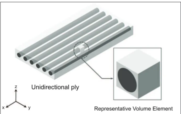
The analysis of composite materials follows a macro, meso, or micromechanical approach. Macromechanics analyzes a laminated plate as a homogeneous anisotropic equivalent plate. In the mesomechanical approach, a laminate is modeled as a stacking sequence of homogeneous layers and interlaminar interfaces (Ladevèze et al., 2005), therefore the prediction of complex behavior, as delamination, can be assessed (Allix, Ladevèze and Corigliano, 1995). The micromechanical analysis goes down to the constituent properties. The object of study on the micromechanical analysis is the representative volume element (RVE), or unit cell, which is the smallest cell capable of representing the overall response of the unidirectional ply to mechanical and thermal loading (Jin et al., 2008). Figure 1 illustrates an example of RVE.
Jin et al. (2008) show the use of three-dimensional
inite element models for obtaining stress distribution on composites. Micromechanical inite element models
provide data to obtain the micro-stresses at the matrix/
iber interface, and great beneits can be reached when a
micromechanical approach is considered. Micromechanics of failure gives a more precise way of composite failure prediction. With the micro-stresses, it is possible to determine the failure initiation in the unidirectional ply (Ha, Huang and Jin, 2008a; Tay et al., 2008; Gotsis, Chamis and Minnetyan, 1998). The material lifetime forecast can be obtained with the use of micromechanics of failure associated with the Accelerated Testing Method (ATM) and Evolution of Damage (Sihn and Park, 2008; Ha, Huang and Jin, 2008b).
The micromechanical theory considers not only the mechanical loads, but also environmental factors, such as thermal loads, as a result of temperature variation and moisture (Hyer and Waas, 2000; Fiedler, Hojo and Ochiai, 2002).
Received: 06/09/11 Accepted: 20/10/11
Unidirectional ply
z
x y Representative Volume Element
Figure 1. Representative volume element in a unidirectional
The inluence of iber arrangements on mechanical behavior
of laminated pates is discussed by Hojo et al. (2009) and Ha, Huang and Jin (2008c). Considerations about the fabrication process are discussed by Aghdam and Khojeh (2003). Studies
with reinforcements other than ibers, such as particles, are
exposed by Zhu, Cai and Tu (2009). Different types of composites, like bulk metallic glasses (Dragoi et al., 2001), metallic matrix composites (Chaboche, Kruch and Pottier, 1998), and smart composites, which include piezoelectric
composites, shape memory alloy (SMA) iber composites,
and piezoresistive composites (Taya, 1999), are also analyzed by micromechanics. Liang, Lee and Suaris (2006) present
the results of a comparison between micromechanical inite
elements modeling and mechanical testing. RVE use in order to represent the composite material is discussed by Sun e Vaidya (1995), and a study of boundary conditions for the unit cell is shown by Xia et al. (2003). From the aeronautical industry to dentistry, a great variety of products can be
beneited from a micromechanical study of a composite
material. Sakaguchi, Wiltbank and Murchison (2003) show micromechanical studies to predict composite elastic modulus and polymerization shrinkage for dental materials.
The micromechanical theory has direct application for the aeronautical industry. Tsai (2008) points out the use of micromechanics to:
• predict macro mechanical properties (stiffness constants, expansion coeficients);
• control the deformation from mechanical and thermal
loads;
• predict a successive ply failure after the irst ply
failure and;
• adjust empirical data by using micromechanical data.
The objective of this paper is to present and to discuss a
methodology in order to obtain the stress ampliication
factors derived from mechanical and thermal loads in a RVE, with the use of two and three-dimensional
inite elements models. Also, this paper aims at accessing stress ampliication factors in an orthotropic unidirectional ply with epoxy matrix, carbon iber, and a perfectly bonded matrix/iber interface, with 60% of iber volume fraction. The materials remain in the linear elastic domain. The inite element models are analyzed
with the commercial software MSC/NASTRAN, version 70.0.6 (MSC, 2011).
STRESS AMPLIFICATION FACTORS
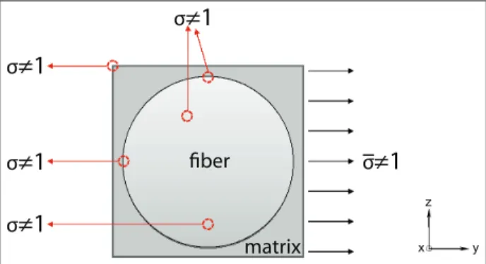
In a micromechanical level, there is a difference between the applied and actual stresses within the
material, mostly because of the dissimilarity on physical properties of the materials. For example, epoxy matrixes present a lower young modulus than the carbon fiber. When a load is applied to a composite material, due to this stiffness difference, the matrix and the fiber tend to show different stresses, resulting in stress concentrations. Therefore, when a unit load is applied to the material, the stresses within the representative volume are no longer unitary, as shown in Fig. 2.
≠1
σ σ
≠1
σ
≠1
fiber
matrix σ
≠1
σ
≠1
z
x y
Figure 2. Differences between micro and macro stresses.
Jin et al. (2008) show that there are ampliication factors
which relates a uniformly distributed unit load (σ, the macro mechanical load) and the internal micromechanical
stresses σ, expressed in Eq. 1:
"MıA T
ı (1)
where,
M and A are matrices that collect the mechanical and
thermal stress ampliication factors, respectively, and ∆T
is the increase of the room temperature.
Considering all stress components, referred to the material coordinate system xyz (the same as 123), Eq. 1 can be expanded by Eq. 2 (Jin et al., 2008):
ı1=ıxx
ı2=ıyy
ı3=ızz
ı4=ıyz
ı5=ızx
ı6=ıxy
=
M11 M12 M13 M14 0 0
M21 M22 M23 M24 0 0
M31 M32 M33 M34 0 0
M41 M42 M43 M44 0 0
0 0 0 0 M55 M56
0 0 0 0 M65 M66 ı
ı1
ı2
ı3
ı4
ı5
ı6
+ A1
A2
A3
A4
A5
A6 ı
¨T
(2)
Mcan be found by applying unidirectional mechanical loads, one at a time. For instance, if a uniformly distributed unit load is applied at x direction, with no thermal load,
ı1 ı2 ı3 ı4 ı5 ı6
=
M11 M12 M13 M14 0 0
M21 M22 M23 M24 0 0
M31 M32 M33 M34 0 0
M41 M42 M43 M44 0 0
0 0 0 0 M55 M56
0 0 0 0 M65 M66
ı
1 0 0 0 0 0
(3)
The resolution of the linear system (Eq. 3) yields Eq. 4:
1
2
3
4
5
6
M11
M21 M31
M41
0 0
ı ı ı ı ı ı
(4)
Therefore, the stress ampliication factors M11, M21, M31 and M41 will be actually the micromechanical stresses σ1,
σ2, σ3 and σ4, respectively. The same procedure can be applied to all directions. Consequently, the methodology consists of the application of uniformly distributed unit loads to the representative volume model. Thus,
the resulting stress at a speciic direction gives the corresponding stress ampliication factor. Since the
stresses at the representative volume vary at each point,
the stress ampliication factor is not constant.
MATERIALS
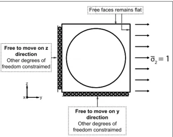
The RVE of a composite material with 60% of iber
volume fraction, subjected to an uniformly distributed load
σ
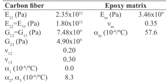
2, is showed in Fig. 3. The iber is represented asa solid cylinder. The mechanical properties of the matrix
and iber are listed in Table 1, where Eij are Young’s moduli, νij are Poisson’s ratios, Gij are shear moduli, and α
the thermal expansion coeficient, referred to the material
coordinate system xyz (the same as 123).
Carbon iber Epoxy matrix
E11 (Pa) 2.35x10¹¹ E
m (Pa) 3.46x10 9 E22=E33 (Pa) 1.80x10¹¹ ν
m 0.35
G12=G13 (Pa) 7.48x10⁹ α m (10
-6/ºC) 57.6 G23 (Pa) 4.90x10⁹
ν12 0.20
ν13 0.30
α1 (10-6/ºC) 0.0
α2, α3 (10-6/ºC) 8.3
Table 1. Mechanical properties of the representative volume element materials (Think Composites, 2011).
NUMERICAL ANALYSIS
Three sets of inite element models are presented and discussed. In the irst set, solid hexahedral elements are used to model the matrix and the iber. The unit cell is
represented as a cube with nondimensionalized edge length (L = 1). Convergence analysis is performed, and stress
ampliication factors for direct, shear, and thermal loads are presented and discussed. Three-dimensional inite elements
are still used in the second set, but the unit cell is no longer modeled as a cube, saving computing efforts. The last set of tests deals with two-dimensional elements. Although they are unable to yield stress concentration factors in transverse
directions, in-plane factors are derived. The inite elements
solutions are compared with results from Super Mic-Mac software (Think Composites, 2011).
Three-dimensional inite element model
The irst set of inite element analysis is applied to a
three-dimensional model, with the eight-node hexahedral
CHEXA Nastran element for the matrix and iber
modeling. The model, including boundary conditions and loads, are further discussed.
Loads and boundary conditions
When a uniformly distributed tension load is applied to a RVE, the unit cell is constrained at its faces, as shown in
Fig. 4, and the free faces must remain lat, as proposed by
Jin et al. (2008), and Xia, Zhang and Ellyin (2003).
To keep free faces lat, rigid elements are applied to
the model. The Nastran rigid element has one master node and one or more slave nodes. The master is the σ2
= 1
y z
x
Figure 3. Representative volume element of a composite
independent one, and it can receive loads. Each slave
node will have the same displacements (in the speciied
direction) of the master one.
Therefore, to keep the right vertical face lat in Fig. 4, a
uniformly distributed unit load σ2 is modeled as a force over only one node. This master node is connected in direction y to the free face nodes (slave nodes) by rigid elements, so all the nodes in this face will have the same displacements in direction y. The nodes in this face must be free at x and z directions (not connected to the master node), in order to move according to the Poisson effect. Rigid body modes are constrained at x=0, y=z=-0.5. Figure 5 shows one model with rigid, spring, and hexahedral elements.
The same procedure must be applied to the others free faces. As it is impossible to enforce two dissimilar
displacements on a node, nodes cannot igure as
dependent on two different master nodes. Therefore, nodes at the edges are connected by spring elements
with high stiffness coeficients. For instance, for face
z=0.5 it is necessary to connect the rigid element to the nodes on the edges parallel to the x-axis. However, these nodes are dependent ones on the rigid elements from faces y=0.5 and y=-0.5. Thus, Nastran spring element Celas2, with high stiffness (say, 1010), is used to connect only the z displacements for that particular
face and, then, this face remains lat. With the Celas2
element, it is possible to connect only one of the degrees of freedom. From faces z=0.5 and z=-0.5, it is connected the z displacements. For faces x=0 and x=1, it is connected the x displacements.
When a uniformly distributed shear load is applied to the RVE, the unit cell is constrained at its faces as shown in Fig. 6, and proposed by Ha et al. (2008). The same procedure already explained is applied here. Rigid body modes are constrained.
Figure 6. Unit cell constraints, subjected to a uniformly distributed shear load σ6= 1.
z
x y
1 6
All degrees of freedom constrained except x translation and x rotation
All degrees of freedom constrained, except x translation and x rotation
x translation and x rotation constrained Free faces remain flat z x y
All degrees of freedom constrained except x translation and x rotation
All degrees of freedom constrained, except x translation and x rotation
Free faces remain flat x translation and
x rotation constrained
σ
6 = 1
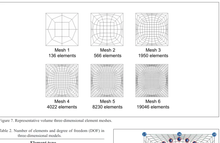
Convergence analysis
To perform a convergence analysis, a uniformly distributed
unit load is applied at direction y. Six inite element meshes are tested (Fig. 7 and Table 2), from a poorly reined 136 element mesh (Mesh 1), to a highly reined 19046 element
mesh (Mesh 6).
In order to present the results of the convergence
analysis, it is necessary to deine a point nomenclature.
The points are numbered according to Tay et al. (2008), as illustrated in Fig. 8. Points 1, 7 and 4 are the best
Free to move on z direction Other degrees of freedom constrained
Free faces remains flat
z
x y
Free to move on y direction Other degrees of freedom constrained
1 2 Free to move on z
direction Other degrees of freedom constrained
Free faces remains flat
z
x y
z
x y
Free to move on y direction Other degrees of freedom constrained 1 2 z x y σ
2
= 1
Free to move on y direction Other degrees of freedom constraimed Free to move on z
direction Other degrees of freedom constraimed
Free faces remains flat
Figure 4. Unit cell constraints, subjected to the uniformly distributed unit load σ2.
z x y
Rigid Element (RBE2)
The face remains flat (same z displacement for
the nodes at face z=0.5)
Rigid Element (RBE2)
The face remains flat (same z displacement for
the nodes at face z=0.5)
Spring Elements (CELAS2)
Same z displacement for the nodes connected by cach spring element at face z=0.5 and z=-0.5
Spring Elements (CELAS2)
Same x displacement for the nodes connected by cach spring element
at face x=0 and x=1
σ
2 = 1 Rigid Element (RBE2)
The face remains flat (same x displacement for
the nodes at face x=1)
suitable to have the results displayed, since they are the points of maximum, minimum, and intermediate
σ
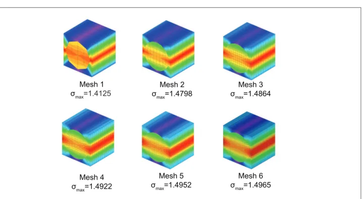
y stresses, respectively. The results of the convergence testing are shown in Figs. 9 and 10.It can be seen that after 4,000 elements (Mesh 4), the
major stress σmax at Point 1 starts to converge to the
value of 1.5. Above 8,000 elements, the results are in the curve asymptotic portion, therefore the chosen mesh is the number 6. Main stresses at points 1, 4 and 7 are compared with results from the Super Mic-Mac Plus (SMM) software (Think Composites, 2011), which are presented in Table 3. SMM has an extensive database
of stress ampliication factors resultant from inite
element analysis for a wide range of physical properties
of iber and matrix, and different volume fractions.
It uses interpolation methods to give the values for
speciications, which are not in the database.
The stress distribution σy (micromechanical) at the RVE is shown in Fig. 11. Since the load is σ2=1, the stress
distribution σy will characterize the stress ampliication factor (M22=1.55).
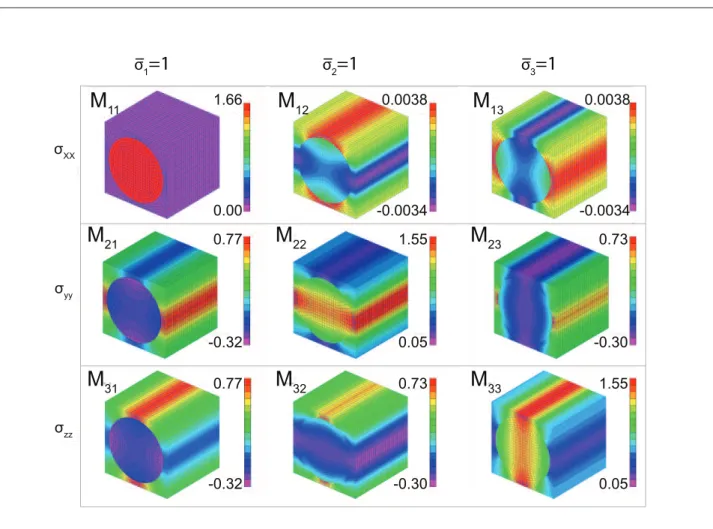
Stress ampliication factors for mechanical loads
The stress ampliication factors with three-dimensional
element meshes are found by applying direct and shear uniformly distributed unit loads at the RVE. As already discussed, the stress contours presented in Figs. 12 and
13 represent the distributions of the stress ampliication factors. Table 4 shows all the 36 stress ampliication factors
at Point 1. These results are compared with solutions by SMM in Tables 5 and 6.
Mesh Element type Total DOF
CHEXA CELAS2 RBE2
1 80 54 2 136 286
2 480 80 6 566 1641
3 1800 144 6 1950 5813
4 3840 176 6 4022 12171
5 8000 224 6 8230 24999
6 18720 320 6 19046 57765
Table 2. Number of elements and degree of freedom (DOF) in three-dimensional models.
Fiber
Matrix
z
y x
Figure 8. Point nomenclature. Figure 7. Representative volume three-dimensional element meshes.
Mesh 1 136 elements
Mesh 2 566 elements
Mesh 3 1950 elements
Mesh 4 4022 elements
Mesh 5 8230 elements
Mesh 1 ımax=1.4125
Mesh 2 ımax=1.4798
Mesh 3 ımax=1.4864
Mesh 4 ımax=1.4922
Mesh 5 ımax=1.4952
Mesh 6 ımax=1.4965
Figure 9. Major stress σmax at the representative volume element.
1,6
1,4
1,2
ıyy
1
0,8
0,6
0,4
0,2
0
0 2000 4000 6000 8000 10000 12000 14000 16000 18000 20000 Point 7 Point 4 Point 1
Figure 10. Stress convergence in the representative volume element.
Point 3D model
(mesh 6) SMM Difference (%)
1 1.49646 1.511233 0.98
4 0.80874 0.810486 0.22
7 0.05139 0.050587 -1.59
Table 3. Stress recovering for representative volume element subjected to a uniformly distributed load
σ
2 = 1.Stress ampliication factors for thermal loads
Stress ampliication factors for thermal loads are obtained by increasing the room temperature by ∆T=1º C. The inite
z
x y
Output Set: MSC/NASTRAN Case 1 Contour: Solid Y Normal Stress
1.55 1.457 1.363 1.269 1.176 1.082 0.988 0.895 0.801 0.707 0.614 0.52 0.426 0.332 0.239 0.145 0.0514
Figure 11. Stress ampliication factor M22.
Figure 12. Stress contours within the RVE, subjected to macro-mechanical tension load. σ
1
=1
σ2=1
σ3=1
0.0038
ıXX
-0.0034 0.0038
-0.0034 1.66
0.00
M
11M
12M
130.73
ıyy
-0.30 1.55
0.05 0.77
-0.32
M
21M
22M
231.55
ızz
0.05 0.73
-0.30 0.77
-0.32
Figure 13. Stress contours within the RVE, subjected to macro-mechanical shear load.
1
ıYZ
0 1
0 1.66
0.00
M
44M
45M
461
ıZX
0 1.55
0.05 1
0
M
54M
55M
561.55
ıXY
0.05 1
0 1
0
M
64M
65M
66σ
4
=1
σ5=1
σ6=1
Stress
σ
1=1σ
2=1σ
3=1σ
23=1σ
31=1σ
12=1σxx 2.43x10
-2 7.74x10⁻¹ -8.00x10⁻² -1.45x10⁻⁵ -2.73x10⁻⁹ -2.20x10⁻⁶
σyy -3.14x10
-3 1.50 -2.62x10⁻¹ 1.19x10⁻⁵ -1.25x10⁻⁹ -7.22x10⁻⁷
σzz 2.89x10
-3 7.33x10⁻¹ 5.14x10⁻² -5.32x10⁻⁵ -1.32x10⁻⁹ -9.73x10⁻⁷
σyz 5.36x10
-8 -7.71x10⁻⁶ 3.59x10⁻⁶ 1.19 -1.07x10⁻¹² -2.37x10⁻¹¹
σzx -2.38x10
-10 1.90x10⁻¹⁰ -1.37x10⁻⁹ 1.26x10⁻⁹ 1.60x10⁻¹ -2.67x10⁻⁵
σxy 5.61x10
-9 -4.69x10⁻⁶ 8.96x10⁻⁷ -2.94x10⁻⁹ -4.85x10⁻⁶ 1.59
Table 4. Stress ampliication factors from Nastran at Point 1, with Mesh 6.
Stress
σ
1=1σ
2=1σ
3=1σ
23=1σ
31=1σ
12=1σxx 2.43x10
-2 7.81x10⁻¹ -8.47x10⁻² -1.15x10⁻¹¹ -1.87x10⁻¹² 5.72x10⁻¹³
σyy -3.22x10
-3 1.51 -2.75x10⁻¹ 1.95x10⁻¹¹ 2.34x10⁻¹² 5.10x10⁻¹²
σzz 2.89x10
-3 7.34x10⁻¹ 5.06x10⁻² -4.29x10⁻¹¹ 5.16x10⁻¹³ 1.13x10⁻¹²
σyz 1.10x10
-12 -5.67x10⁻¹¹ 1.98x10⁻¹¹ 1.21 9.42x10⁻¹⁴ 1.15x10⁻¹³
σzx -4.05x10
-14 2.24x10⁻¹² -4.81x10⁻¹³ 3.63x10⁻¹² 1.59x10⁻¹ -2.53x10⁻¹¹
σxy 2.27x10
-15 -4.80x10⁻¹³ 3.34x10⁻¹³ -1.75x10⁻¹² 9.80x10⁻¹² 1.59 Table 5. Stress ampliication factors from SMM at Point 1.
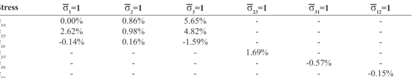
Stress
σ
1=1σ
2=1σ
3=1σ
23=1σ
31=1σ
12=1σxx 0.00% 0.86% 5.65% - -
-σyy 2.62% 0.98% 4.82% - -
-σzz -0.14% 0.16% -1.59% - -
-σyz - - - 1.69% -
-σzx - - - - -0.57%
-σxy - - - -0.15%
Finite element model simpliications
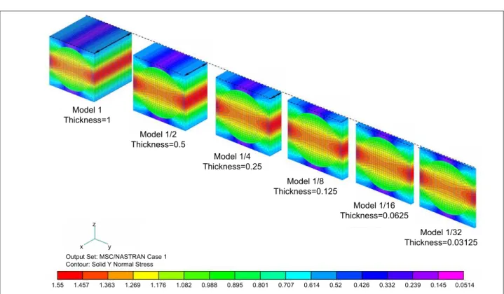
It is notable that all the results are constant within the element along the x axis, as illustrated in details in Fig. 15. This suggests that: a courser three-dimensional mesh can be used at x direction or the model does not need necessarily to be three-dimensional.
A series of model simpliications is carried out. The irst part focuses on three-dimensional simpliications by
reducing the number of elements in x direction. The cubic
inite element model showed in Fig. 5 is reduced on its
half and the resulting model is called Model 1/2. Those
model simpliications are carried out up to Model 1/32, as
presented in Fig. 16.
The stress ampliication factors found with Models 1 to
1/32 are virtually the same, as long as the mesh stays three-dimensional (solid elements). For example, the difference between the full size model and the one with 1/32 of thickness (Model 1/32) is, in the worst scenario, 0.01%.
The next step of this study is to verify the differences between the results of the three-dimensional Model 1/32 and two-dimensional ones. Two different two-dimensional Nastran elements are used: the four-node (linear) quadrilateral membrane CQUAD4 element and the eight-node (parabolic) quadrilateral membrane CQUAD8.
Figure 17 shows σy stress contours for the RVE subjected to a uniformly distributed unit load σ2. The correspondent
stress ampliication factors M22 are listed in Table 8. Table 9 shows that two-dimensional models fail in calculating accurate in-plane results.
CONCLUSION
In this paper, a inite element procedure is presented to
access internal stresses in micromechanical analysis of
composites materials, with unidirectional ibers. First, three-dimensional inite element models of a RVE
are idealized and modeled in Nastran, with CHEXA (hexahedral), CELAS2 (spring), and rigid (RBE2) elements. Convergence analysis is performed. Stress
ampliication factors are derived within a RVE under
tension, shear, and thermal load. Then, two-dimensional Nastran models are also proposed.
2.2x10⁵
A
1ΔT = 1°C
A
2
A
3
-2.5x10⁵
2.2x10⁵
-2.5x10⁵
2.2x10⁵
-2.5x10⁵
σ
xx
σ
yy
σ
zz
Figure 14. Stress contours within the RVE, subjected to thermal load ∆T = 1ºC.
Stress Model SMM Difference
(%)
σxx -1.92x10
5 -1.90x10⁵ -0.74
σyy 2.06x10
5 2.11x10⁵ 2.59
σzz -1.90x10
5 -1.90x10⁵ 0.17
σyz -3.63 -1.75x10
-5
-σzx -1.02x10
-5 7.89x10⁻⁷
-σxy -5.92x10
-1 -1.20x10⁷
-Table 7. Stress ampliication factors at Point 1 for thermal load.
z
x y
1.55 1.457 1.363 1.269 1.176 1.082 0.988 0.895 0.801 0.707 0.614 0.52 0.426 0.332 0.239 0.145 0.0514
Output Set: MSC/NASTRAN Case 1 Contour: Solid Y Normal Stress
Figure 15. Representative volume element in a cutaway view on
The presented two-dimensional models fail in providing
accurate in-plane stress ampliication factors. Good estimation for internal stress ampliication factors is
achieved with three-dimensional models. Good results
can be derived with a single transverse layer of solid
inite elements, an important feature for nonlinear
analyses. The good performance of the presented three-dimensional models shows that good estimates for stress
!
z
Output Set: MSC/NASTRAN Case 1 Contour: Solid Y Normal Stress
1.55 1.457 1.363 1.269 1.176 1.082 0.988 0.895 0.801 0.707 0.614 0.52 0.426 0.332 0.239 0.145 0.0514 x y
Model 1/32 Thickness=0.03125 Model 1/16
Thickness=0.0625 Model 1/8
Thickness=0.125 Model 1/4
Thickness=0.25 Model 1/2
Thickness=0.5 Model 1
Thickness=1
Figure 16. Three-dimensional models for RVE, subjected to macro-mechanical unit load σ2(σy contours).
Figure 17. Stress ampliication factors M22 with: (a) three-dimensional Model 1/32 (2984 DOF); (b) linear membrane elements (1464
DOF); (c) parabolic membrane elements (4368 DOF).
1.55
1.457
1.269
0.988
0.426
0.0514
(a) (b) (c)
1.589
1.496
1.311
1.033
0.477
0.107
1.595
1.502
1.316
1.036
0.477
0.105
Stress
σ
1=1σ
2=1
σ
3=1σyy 1.545112 0.152274
-σzz 0.480766 0.104816
-σyz - - 1.287447
Table 8. Stress ampliication factors with parabolic membrane
elements.
Stress
σ
1=1σ
2=1σ
3=1σyy 3.25% 41.92%
-σzz 34.38% 103.97%
-σyz - - 8.17%
Table 9. Differences between stress ampliication factors found with
ampliication factors can be derived for other than the
presented composite (with another volume fraction, or
for bidirectional ibers composite), and also to access strain ampliication factors.
REFERENCES
Allix, O., Ladevèze P., Corigliano, A., 1995, “Damage analysis of interlaminar fracture specimens”, Composite Structures, Vol. 31, No. 1, p. 61-74. doi:10.1016/0263-8223(95)00002-X
Aghdam, M., Khojeh, A., 2003, “More on the effects of thermal residual and hydrostatic stresses on yelding behavior of unidirectional composites”, Composite Structures, Vol. 62., No. 3-4, p. 285-90.
Boeing. 787 Dreamliner – Program Fact Sheet. Retrieved in 2010 August 2, from: http://www.boeing.com/ commercial/787family/programfacts.html.
Chaboche, J.L., Kruch, S., Pottier, T., 1998, “Micromechanics versus Macromechanics: a combined approach for metal matrix composites constitutive modeling”, European Journal of Mechanics, Vol. 17, No. 6., p. 885-908.
Dragoi, D., et al., 2011, “Investigation of thermal residual stresses in tungsten-fiber/bulk metallic glass matrix composites”, Scripta Materialia, Vol. 45, No. 2, p. 245-52.
Fiedler, B., Hojo, M., Ochiai, S., 2002, “The influence of thermal residual stresses on the transverse strength of CRFP using FEM. Composites Part A: Applied Science and Manufacturing”, Vol. 33., No. 10, p. 1323-6.
Gotsis, P.K., Chamis, C.C., Minnetyan, L., 1998, “Prediction of Composite laminate fracture: micromechanics and progressive fracture”, Composites Science and Technology, Vol. 58, No. 7, p. 1137-49.
Ha, S.K., Huang, Y., Jin, K.K., 2008a, “Effects of Fiber Arrangement on Mechanical Behavior of Unidirectional Composites”, Journal of Composites Materials, Vol. 42, No. 18, p. 1851-71.
Ha, S.K., Huang, Y., Jin, K.K., 2008b, “Life Prediction of Composites using MMF and ATM”. In: Tsai, S., 2008, “Strength and Life of Composites”, Stanford, Department of Aeronautics & Astronautics of Stanford University.
Ha, S.K., Huang, Y., Jin, K.K., 2008c, “Micro-Mechanics of Failure (MMF) for Continuous Fiber Reinforced
Composites”, Journal of Composites Materials, Vol. 42, No. 18, p. 1873-95.
Hojo, M., et al., 2009, “Effect of iber array irregularities
on microscopic interfacial normal stress states of transversely loaded UD-CFRP from viewpoint of failure initiation”, Composites Science and Technology, Vol. 69, No. 11-2, p. 1726-34.
Hyer, M.W., Waas, A.M., 2000, “Micromechanics of Linear Elastic Continuous Fiber Composites”, In: Kelly, A., Zweben, C., 2000, “Comprehensive Composite Materials”, Elsevier Science Publishers.
Jin, K.K., et al., 2008, “Distribution of micro stresses and interfacial tractions in unidirectional composites”, Journal of Composite Materials, Vol. 42, No. 18.
Ladevèze, P., et al., 2005, “Micro and meso computational damage modellings for delamination prediction”, ICF XI - 11th International Conference on Fracture.
Liang, Z., Lee, H.K., Suaris, W., 2006, “Micromechanics-based constitutive modeling for unidirectional laminated composites”, International Journal of Solids and Structures, Vol. 43, No. 18-9, p. 5674-89.
Msc Software, 2011, “MD Nastran: Integrated, Multidiscipline CAE Solution”, Retrieved in 2011 March 23, from http://www.mscsoftware.com/Products/ CAE-Tools/MD-Nastran.aspx.
Sagushi, R., Wiltbank, B., Murchison, C., 2004, “Prediction of composite elastic modulus and polymerization shrinkage by computational micromechanics”, Dental Materials, Vol. 20, No. 4, p. 397-401.
Sihn, S., Park, J. W., 2008, “An Integrated Design Tool for Failure and Life Prediction of Composites”, Journal of Composites Materials, Vol. 42, No. 18, p. 1967-88.
Sun, C. T., Vaidya, R. S., 1996, “Prediction of Composite Properties from a Representative Volume Element”, Composites Science and Technology, Vol. 56, No. 2, p. 171-9.
Tay, T.E., et al., 2008, “Progressive Failure Analysis of Composites”, Journal of Composites Materials, Vol. 42, No. 18, p. 1921-66.
Think Composites, 2011, “Super Mic-Mac – a new preliminary design tool for composites”, Retrieved in 2011 March 23, from http://www.thinkcomposites.com/ index_eng.php.
Tsai, S., 2008, “Strength and Life of Composites”, 1st ed, Stanford: Department of Aeronautics & Astronautics of Stanford University.
Xia, Z., Zhang, Y., Ellyin, F., 2003, “A uniied boundary
conditions for representative volume elements of composites and applications”, International Journal of Solids and Structures, Vol. 40, No. 8, p. 1907-21.