Federal University of Ceará Center of Technology
Department of Chemical Engineering
Leonardo de Pádua Agripa Sales
An integrated optimization and
simulation model for refinery
planning including external loads and
product evaluation
Um modelo integrado de simulação e otimização para o planejamento de refinarias incluindo cargas externas e
avaliação de produtos
Leonardo de Pádua Agripa Sales
An integrated optimization and simulation model
for refinery planning including external loads and
product evaluation
Bachelor Thesis submitted to the
Department of Chemical Engineering
in partial fulfillment of the requirements
for the degree of Bachelor of Science in
Petroleum Engineering at the Federal
University of Ceará.
Dados Internacionais de Catalogação na Publicação Universidade Federal do Ceará
Biblioteca Universitária
Gerada automaticamente pelo módulo Catalog, mediante os dados fornecidos pelo(a) autor(a)
S155a Sales, Leonardo de Pádua Agripa.
An integrated optimization and simulation model for refinery planning including external loads and product evaluation / Leonardo de Pádua Agripa Sales. – 2016.
21 f. : il. color.
Trabalho de Conclusão de Curso (graduação) – Universidade Federal do Ceará, Centro de Tecnologia, Curso de Engenharia de Petróleo, Fortaleza, 2016.
Orientação: Prof. Dr. Bruno de Athayde Prata.
Coorientação: Prof. Dr. Francisco Murilo Tavares de Luna.
1. Refinery optimization. 2. Production planning. 3. Decision support systems. 4. Nonlinear programming. I. Título.
Leonardo de Pádua Agripa Sales
An integrated optimization and simulation model for refinery planning including external loads and product evaluation
Bachelor Thesis submitted to the
Department of Chemical Engineering
in partial fulfillment of the requirements
for the degree of Bachelor of Science in
Petroleum Engineering at the Federal
University of Ceará.
Approved by:
Prof. Dr. Bruno de Athayde Prata (Advisor) Federal University of Ceará
Prof. Dr. Francisco Murilo Tavares de Luna (Advisor) Federal University of Ceará
Prof. Dr. Tibérius de Oliveira e Bonates Federal University of Ceará
Prof. Dr. Anselmo Ramalho Pitombeira Neto Federal University of Ceará
Resumo
D
crescente preocupação com o planejamento da produção das refinarias.adas as incertezas da indústria do petróleo a nível mundial, existe uma Embora existam modelos para este planejamento, eles são bastante limitados em sua utilização, pois abrangem poucos cenários de operação. Este estudo descreve uma abordagem integrada envolvendo a simulação de unidades e a otimização não-linear das operações deblending a fim de obter um planejamento da produção que maximize o lucro obtido. O problema é modelado através da interface do software LINGO 16.0 e é resolvido utilizando-se o Global Solver do aplicativo. Um estudo de caso com base na Refinaria de Paulínia é apresentado e as cargas externas, a adição de produtos e a avaliação do preço dos produtos são estudadas, alcançando a solução ótima global para o blending em menos de um segundo em todos oscenários analisados, garantindo assim a utilidade do modelo no planejamento da produção de refinarias, sendo também importante para as análises de sensibilidade e a determinação dos pontos de equilíbrio para cargas externas e novos produtos. Os resultados apontam que esta nova abordagem tem um potencial considerável para obter ganhos significativos em termos de planejamento e aumento nos lucros. A flexibilidade do modelo aliada com a sua rápida obtenção de boas soluções são destaques da abordagem proposta.
Abstract
B
about their planning operations. Although models for this planning exist, theyecause of its potential benefits, petroleum refineries are increasingly concerned are bounded into their usefulness. This study describes an integrated approach involving nonlinear optimization and simulation of refinery units in order to obtain a production planning for a given refinery that maximizes profit. The problem is modeled through the LINGO 16.0 software interface and is solved using LINGO’s Global Solver. A case study pertaining Refinaria de Paulínia (REPLAN) is proposed, and external loads, product adding, and product pricing is studied, achieving global optimum solution for the blending on less than a second on every case, assuring the model usefulness into refinery planning and being important to sensitivity analyses and the determination of break-even points of external loads and of new products. The results indicate that this new approach has a considerable potential for achieving significant gains in terms of planning and profit increase. The flexibility of the model allied with its quick generation of good solutions is highlighted.Acknowledgments
Though only my name appears on the cover of this monograph, many people have contributed to its production. I owe my gratitude to all those people who have made this dissertation possible and because of whom my undergraduate experience has been one that I will cherish forever.
My deepest gratitude is to my advisor over my academic life, Dr. Bruno Prata. I have been amazingly fortunate to have an advisor who gave me the freedom to explore on my own, and at the same time the guidance to recover when my steps faltered. Bruno not only taught me about academic subjects, he taught me how to be a better human being. His patience and support helped me overcome many situations and finish this dissertation. I would like to thank you very much for your support and understanding over these years.
My advisor Dr. Murilo Tavares has been always there to listen and advise. I am deeply grateful to him for the long discussions that helped me sort out the technical details of my work. Without his assistance and dedicated involvement in every step throughout the process, this monograph would have never been accomplished. I am also thankful to him for his careful comments on the revisions of this manuscript.
Dr. Tibérius Bonates insightful comments about technical issues of this dissertation were thought-provoking. I feel thankful and indebted to him for his share of knowledge, for holding me to a high research standard, for his pacience and kindly assistance on this study.
My sincere thanks also goes to Dr. Ernesto Nobre, who provided me an opportunity to join his team as an assistant researcher at the Logistics and Infrastructure Networks laboratory. Without his precious support it would not be possible to conduct this research.
I thank my girlfriend Kássia Carvalho for all her love and support.
Contents
List of Figures v
List of Tables vi
List of Symbols vii
List of Abbreviations x
1 Introduction 1
2 Problem Description 4
3 Models and Procedures 6
4 Case Study 14
5 Conclusions 23
List of Figures
1 General refinery scheme . . . 5
2 Model of REPLAN refinery . . . 16
3 Sensitivity analysis for gasoline production . . . 20
4 Sensitivity analysis for petrochemical naphtha production . . . 20
5 Sensitivity analysis for fuel oil export production . . . 21
List of Tables
1 Unit types and their processing capacities . . . 14
2 Benchmark crudes and their percentage received . . . 15
3 Percentage of products sold by categories . . . 17
4 Computational time of global optimizations . . . 18
5 External loads behavior . . . 19
6 New product addition . . . 22
List of Symbols
Indexes and sets
c ∈ C set of available campaigns for distillation in the refinery.
d ∈ D subset of distillation units in the refinery.
e ∈ E set of available campaigns for other processes in the refinery. i ∈ I set of intermediate fractions.
k ∈ K subset of intermediate fractions produced at distillation.
o ∈ O set of oils used in the refinery.
p ∈ P set of products produced in the refinery.
t ∈ T subset of intermediate fractions produced at other processes. u ∈ U set of processing units in the refinery.
w∈ W subset of other processing units in the refinery.
Constants
CDSd operational cost of distillation unit d ($/m3).
CDT distillation unit operating cost ($). CPR unit operating cost ($).
CPSw operational cost of unit w ($/m3).
CTSk current external intermediate k load price ($/m3).
EXPiwe expansion of intermediate i processed through campaign e in
unit w (% volume).
FOCi octane enhance factor of intermediate i.
IVIi viscosity index of intermediate i produced. The viscosity blending index
is calculated as seen on Bueno (2003): IV I = ln V ISCOSIT Y(cSt)
ln(V ISCOSIT Y(cSt)·1000)
IVImax,p maximum viscosity index of product p.
IVImin,p minimum viscosity index of product p.
IVIodck viscosity blending index at 50◦C of intermediatek, which belongs to oil o,
processed through campaign c in distillation unitd.
IVIwte viscosity index of intermediate t, processed through campaign e in unitw.
IVITk viscosity index of intermediate k from an external load.
MKCmax,p maximum market of product p supplied (m3).
MKCmin,p minimum market of product p supplied (m3).
NPGmax maximum distilled naphtha composition in gasoline (% volume).
NPGmin minimum distilled naphtha composition in gasoline (% volume).
OCTi octane rating of intermediate i produced.
OCTmin,p minimum octane rating of product p.
OCTodck octane rating of intermediate k, which belongs to oil o, processed through campaign c in distillation unitd.
OCTTk octane rating of intermediate k from an external load.
PDTk volume of intermediate k produced in distillation (m3).
POSo current oil o price ($/m3).
PPRt volume of intermediate t produced in a process unit (m3).
PPSp current product p price ($/m3).
QDTmax,d maximum distillation volume of unit d (m3).
QDTmin,d minimum distillation volume of unit d (m3).
QDTodc volume of distilled oil o, processed through campaign c in distillation
unit d (m3).
QDTOo volume of oil o processed in the refinery (m3).
QDTUd volume processed in distillation unit d (m3).
QPRiwe volume of intermediate i processed
in unit w through campaign e (m3).
QPRmax,w maximum process volume of unit w (m3).
QPRmin,w minimum process volume of unit w (m3).
QPRUw volume processed in unit w (m3).
RDTodck volumetric fraction of intermediate k, which belongs to oil o, processed
through campaign c in distillation unitd (% volume).
RPRiwte volumetric fraction of processed intermediate t, which belongs to
inter-mediate i, processed through campaign e in unit w (% volume). RPRwie sulfur transfer factor for intermediate i, processed through campaign e
in unit w (% weight).
SPCi specific mass of intermediate i produced (kg/m3).
SPCodck specific mass of intermediate k, which belongs to oil o, processed
through campaign c in distillation unitd (% volume).
SPCwte specific mass of intermediate t, processed through campaign e
in unit w (kg/m3).
SPCw specific mass of the load in unit w (kg/m3).
SPCTk specific mass of intermediate k from an external load (kg/m3).
SULi sulfur content of intermediate i produced (% weight).
SULmax,p maximum sulfur content of product p (% weight).
SULodck sulfur content of intermediate k, which belongs to oil o, processed
through campaign c in distillation unitd (% weight).
SULtw sulfur content of intermediate t produced in unit w (% weight).
SULt sulfur content of intermediate t (% weight).
SULw sulfur content of the load in unit w (% weight).
SULTk sulfur content of intermediate k from an external load (% weight).
VOLmax,o maximum oil o volume (m3).
VOLmin,o minimum oil o volume (m3).
VTRi volume transferred of intermediate i to the refinery (m3).
Decision variables
ESTi volume of intermediatei that is stocked (m3).
IVIp viscosity index of the product p obtained by the blending
of intermediates.
NPG distilled naphtha composition in gasoline (% volume).
OCTp octane rating of the productp obtained by the blending of intermediates.
PBLp volume of the productp obtained by the blending of intermediates (m3).
QBLi,p volume of intermediatei transferred to product p (m3).
SPCp specific mass of the product p obtained by the blending of
intermediates (kg/m3).
SULp sulfur content of the productp obtained by the blending of
intermediates (% weight).
RVP income generated by product sales ($).
List of Abbreviations
Intermediates and products
AR1 fraction produced on distillation unit (distillation range temperature between 440◦C and 560◦C) routed to catalytic cracking unit.
GHK fraction produced on delayed coking unit routed to catalytic cracking unit, catalytic hydrotreatment unit and blending pools.
GLK fraction produced on delayed coking unit routed to catalytic cracking unit and catalytic hydrotreatment unit.
GMK fraction produced on delayed coking unit routed to catalytic cracking unit, catalytic hydrotreatment unit and blending pools.
GO1 fraction produced on distillation unit (distillation range temperature between 405◦C and 440◦C) routed to catalytic cracking unit.
HD1 fraction produced on distillation unit (distillation range temperature between 306◦C and 405◦C) routed to process units and blending pools. HDI fraction produced on catalytic hydrotreatment unit routed to
blending pools.
HN1 fraction produced on distillation unit (distillation range temperature between 140◦C and 170◦C) routed to blending pools.
HNK fraction produced on delayed coking unit routed to catalytic hydrotreatment unit.
KR1 fraction produced on distillation unit (distillation range
temperature between 170◦C and 225◦C) routed to blending pools. LCO fraction produced on catalytic cracking unit routed to catalytic
hydro-treatment unit and blending pools.
LN1 fraction produced on distillation unit (distillation range temperature between 20◦C and 140◦C) routed to blending pools.
LNK fraction produced on delayed coking unit routed to catalytic cracking unit.
LP1 fraction produced on distillation unit (distillation range temperature up to 20◦C) added to the final product LPG.
LPC fraction produced on catalytic cracking unit added to the final product LPG.
LPG Liquefied Petroleum Gas.
LPK fraction produced on delayed coking unit added to the final product LPG.
NFC fraction produced on catalytic cracking unit routed to blending pools. OLD fraction produced on catalytic cracking unit routed to blending pools. VR1 fraction produced on distillation unit (distillation range temperature
beyond 560◦C) routed to delayed coking unit and blending pools.
Refinery units
CDU Crude Distillation Unit. DCU Delayed Coking Unit.
FCC Fluid Catalytic Cracking unit. HDT Hydrotreatment unit.
Distillation campaigns
ASPHALT campaign that separates heavy vacuum residuum for asphalt production.
HSC High Sulfur Content campaign, which separates intermediates with high sulfur content.
NORMAL campaign that does not separate by any characteristic of the intermediate.
RATCRACK campaign that separates atmospheric residuum.
Other
BEP break-even point.
Chapter
1
Introduction
A refinery consists of multiple processes that divide, blend and react hundreds of hydrocarbon types, inorganic and metallic compounds, with the purpose of obtaining commercial products. In a refinery, the required characteristics of a product are fixed. However, crude oil has characteristics that depend on crude origin. Then, if the crude oils change and products are fixed, refineries must adapt their operational configurations.
In addition, a refinery suffers from rising oil prices, advances in environmental restrictions and pressure from consumers for lower prices, thus working with narrow profit margins. It is vital for a refinery to operate as nearly as possible on its optimal level and to seek opportunities for increasing the profits. However, without some form of computational modeling, an optimum production plan that maximizes profit is hard to obtain. These are the reasons for virtually every refiner nowadays to use advanced process engineering tools to improve business results (MORO, 2003).
Since the invention of the Simplex algorithm by Dantzig in 1947, many computational mathematical models have been applied to solve specific subjects of a refinery, such as gasoline blending, refinery scheduling and planning (BODINGTON; BAKER, 1990). Láng et al. (1991) present an algorithm and a FORTRAN program for modeling crude distillation and vacuum columns. The proposed approach presents a good convergence and low memory requirements. Nevertheless, the proposed algorithm cannot guarantee the optimality of the generated solutions.
2 Chapter 1. Introduction
scenarios of Presidente Bernardes Cubatão refinery (RBPC) and Henrique Lage refinery (REVAP), and then comparing the results with the current situation of both refineries. The model has a great potential for increasing profitability embedded in the planning activity, reaching several millions of dollars per year.
Pinto and Moro (2000) state that the existing commercial software for refinery production planning, such as RPMS (Refinery and Petrochemical Modeling System) and PIMS (Process Industry Modeling System) are based on very simple models that are mainly composed of linear relations. The production plans generated by these tools are interpreted as general trends as they do not take into account more complex process models and/or nonlinear mixing properties.
Process unit optimizers based on nonlinear complex models that determine optimal values for the process operating variables, as seen in More et al. (2010), have become increasingly popular. However, most are restricted to only a portion of the plant. Furthermore, single-unit production objectives are conflicting and therefore contribute to suboptimal and even inconsistent production objectives (PINTO; MORO, 2000). Li et al. (2006) present a linear programming model for integrated optimization of refining and petrochemical plants, determining on a case study that the profit has an about $1.0 million increase per month comparing to the case without optimization. They conclude that integrative optimization of refining and petrochemical plants is a developing trend and it should attract more concern in the future.
Moro and Pinto (2004) present a review of the technology of process and production optimization in the petroleum refining industry. An important conclusion of this study is related to the improvement necessity of the optimization approaches. Although the mathematical programming models can be useful in refining and petrochemical companies, these approaches still lack many real characteristics of the modeled systems to be widely applied in the corporate business. A nonlinear approach represents the real nature of the processing units, as stated by Alattas, Grossmann and Palou-Rivera (2011). Therefore, a linear model would result in a precision loss in the model results (LI; HUI; LI, 2005).
3
approach can capture the dynamic nature of the real system. In addition, the optimization model can consider multiple objectives.
Gueddar and Dua (2011) present a compact nonlinear refinery model based on input-output data from a process simulator, emphasizing the continuous catalytic reformer and naphtha splitter units. These authors propose artificial neural networks to deal with the complexity related with large amounts of data. However, there is not a focus on global optimization issues in the proposed approach.
Menezes, Kelly and Grossmann (2013) develop a fractionation index model (FI) to add nonlinearity to the linear refinery planning models. The FI model is developed as a more accurate nonlinear model for the complex crude distillation unit (CDU) than the fixed yield or the swing cuts models. The results are compared to the common fixed yield and swing cuts models, concluding that the FI refinery planning model predicted higher profit based on different crude purchase decision.
We can conclude that there is a lack of refinery-wide planning that considers the many processes and its nuances, especially when using nonlinear models. In addition, the studies do not employ other methods to increase profit besides optimization and modeling.
In this context, this study aims to obtain a production planning for the profit maximization in a refinery, simulating and optimizing the blending operations through a nonlinear programming model proposed by Bueno (2003) that considers crude distillation units (CDU), fluid catalytic cracking units (FCC), hydrotreatment units (HDT) and delayed coking units (DCU). It is proposed an addition to the Bueno (2003) model that takes into account the acquisition of external intermediate loads for blending into the refinery, allowing a realistic planning. This monograph also proposes methods combined with optimization, such as sensitivity analysis and the determination of break-even points of external loads and of new products, aiming to enhance the refinery planning and to increase its profit.
Chapter
2
Problem Description
A typical refinery carries out several physicochemical processes to obtain the required products. We can describe the general planning model of a refinery assuming the existence of several processing units, producing a variety of intermediate streams with different properties that can be blended to constitute the desired kinds of products. A general scheme of a refinery is presented in Figure 1. The n distillation units receive the oil,
distilling it into multiple intermediates that are going to possibly receive a load from external sources and/or be transformed into other intermediates through the m process units. The intermediates will be mixed on the k blending pools available, leaving the refinery as one of thew specified products. The relation between the inputs and outputs,
plus the operational and intermediate costs, leads to the refinery profit.
Usually, in a refinery both oil acquisition and product selling are predefined by the organization. Therefore, a minimum and a maximum market for a product, and the volume of oil acquired are usually predefined in order to meet the organization expectations (BUENO, 2003). The refineries must check the feasibility of this planning, and in case of adversities (lack of supply, broken equipment, etc.), it must match to the new reality. The volume of each oil type acquired is the most important information, since it will affect the entire refining system.
5
Figure 1: General refinery scheme.
Distil-lation
Unit
2
Process unit 2 Process unit 3 Process unit 1 Process unit m Blending pool 1 Blending pool 2 Blending pool 3 Blending pool kDistil-lation
Unit
n
Distil-lation
Unit
1
...
...
...
Intermediate 2 Intermediate 1 Intermediate 5 Intermediate 4 Intermediate 6 Intermediate 7 Oil type 1Oil type 2 Oil type 3
...
Product 1 Product 2 Product 3 Product 4 Product 5 Product w Intermediate q...
Intermediate 8 Intermediate 1 Load...
Intermediate 7 Load Intermediate q LoadOil type 4 Oil type 5
Oil type 6 Oil type 7 Oil type 8 Oil type 9 Oil type 10
Oil type x-k
Oil type x
Chapter
3
Models and Procedures
We intend to obtain a production planning in a given refinery that maximizes profit, considering operational constraints. It is assumed an ideal mixture, as the compounds in the petroleum are chemically similar, for easily adding intermediate volumes, thus lowering computational times. Hereafter, the notation used for the design of the model will be presented.
Similar to Bueno (2003), Pitty et al. (2008) and Koo et al. (2008), in this study we propose an integrated approach, which is composed of a simulation-optimization model and graphical interfaces. The simulation encompasses all distillation and process units, while the optimization encompasses the intermediate volume in each blending pool (QBLp), which is optimized for the objective of maximum profit, having as constraints
the entire scheme of the refinery and the market restrictions.
In this study we develop a model whose data is imported and exported using a user-friendly interface. Such developments have proven to be of capital importance for efficiently optimizing production planning and scheduling by accurately addressing quality issues, as well as plant operational rules and constraints, in a straightforward way (JOLY, 2012). Through Excel’s interface, the necessary data to solve the model is inserted. The data is merged into the mathematical model and then the LINGO solver finds optimum values. These optimum values are exported to Excel and translated into information, which enables analysis by decision-making industry professionals.
The sensitivity analysis works by varying one parameter from the model. After solving the modified model, the results are collected and the impact of the parameter variation is analyzed.
7
transfer of external intermediate loads to the refinery. The model is limited to adding distilled intermediates that go directly to blending, since adding intermediates that go to process units would largely increase the complexity of the model. The properties of the load must be specified, since it will affect the blending.
The objective function (1) maximizes the profit of a refinery by subtracting the income (product sale) from the purchase of crude oil, operational costs of units, and external intermediate loads costs. The first term is the income generated by the products sold. The second term represents the associated cost with crude oil purchase. The third term refers to total operational cost of distillation units in the refinery. The fourth term refers to total operational cost of processes units, except distillation, in the refinery. The fifth term refers to the cost of purchasing the external loads of intermediates transferred to the refinery. All symbols used in the equations are explained in the List of Symbols.
The set of constraints (2a), (2b), and (2c) are similar. The first refers to the volume of distilled oil o in distillation unit d, the second refers to the total volume distilled in unit d, and the third the total volume distilled of oil o. Constraint (3) refers to the total volume of crude oil that enters the refinery.
The set of constraints (4) refers to the volume of distilled oil (intermediate) k that
leaves the distillation process plus the volume of the external load of intermediate k
transferred into the refinery (VTRi). The sets of constraints (5), (6), (7), and (8)
determine the specific mass, sulfur content, viscosity index and octane rating of each intermediate k, considering the addition of the external intermediate load.
Similar to (2b), the set of constraints (9) refers to the total volume processed in unit
w. The sets (10) and (11) represents the specific mass and sulfur content in each unit w, which is related to each intermediate that enters the unit.
The set of constraints (12) determines the volume fraction of intermediate t, which is the product of a reaction of intermediate i. As the reaction occurs, there is some
expansion, especially at FCC. Along the expansion, there are changes in sulfur content, being redistributed through the produced intermediates. The expansion of intermediate
i in unit w is determined in the set of restrictions (13). The sulfur content in the
intermediate t is determined by sets (14) and (15).
The intermediates produced or distilled i are either blended or stocked. Set of
8 Chapter 3. Models and Procedures
The sets of constraints (22), (23), (24), and (25) establish the expenses of distillation operation cost, processing unit operation cost, crude oil purchase, and external intermediate load purchase, respectively. Set (26) determines the income generated by product sales. The set (27) determines the distilled naphtha proportion on gasoline produced.
The set of constraints (28) refers to the maximum and minimum market restraints for each oil acquisition. Sets of constraints (29) and (30) determine the capacity limits of distillation and non-distillation units respectively. Sets of constraints (31), (32), and (33) establish the upper and/or lower proprieties for sulfur content, octane rating, and viscosity index, respectively for each product. Similar to set (28), set of constraints (34) refers to the maximum and minimum market restraints for the specific product p sale. Equation
(35) restricts the maximum and minimum distilled naphtha proportion in gasoline.
Equations (4, 5, 6, 7, 8, and 21) compute the contribution of external intermediate loads into each one of the proprieties. Equation (25) determines the cost of external intermediate loads. Equations (27) and (35) restrict the maximum and minimum distilled naphtha proportion in gasoline.
Objective Function
max Z =X
p∈P
P P Sp·P BLp−
X
o∈O
P OSo·QDTo−
X
d∈D
CDSd·QDTd
− X
w∈W
CP Rw·QP Rw−
X
i∈I
CT Si·V T Ri (1)
Balance Equations
Oil volume in distillation units
QDTo,d =
X
c∈C
QDTo,d,c ∀ o∈O, d∈D (2a)
QDTd =
X
o∈O
9
Oil volume by type
QDTo =
X
d∈D
QDTo,d ∀ o ∈O (2c)
Total oil volume
QDT =X
o∈O
QDTo (3)
Volume of distillate k
P DTk =V T Rk+
X
o∈O
X
d∈D
X
c∈C
QDTo,d,c·RDTo,d,c,k ∀ k ∈K (4)
Specific mass, sulfur content, viscosity index, and octane rating of distillate k
SP Ck=
V T Rk·SP CTk+ P o∈O
P
d∈D
P
c∈C
QDTo,d,c·RDTo,d,c,k·SP Co,d,c,k
P DTk
∀ k∈K (5)
SU Lk=
V T Rk·SP CTk·SU LTk
P DTk·SP Ck
+
P
o∈O
P
d∈D
P
c∈C
QDTo,d,c·RDTo,d,c,k·SP Co,d,c,k ·SU Lo,d,c,k
P DTk·SP Ck
∀ k∈K
(6)
IV Ik=
V T Rk·IV ITk+ P o∈O
P
d∈D
P
c∈C
QDTo,d,c·RDTo,d,c,k·IV Io,d,c,k
P DTk
∀ k∈K (7)
OCTk=
V T Rk·OCT Tk+
P
o∈O
P
d∈D
P
c∈C
QDTo,d,c·RDTo,d,c,k·OCTo,d,c,k
P DTk
10 Chapter 3. Models and Procedures
Volume of all intermediates processed in unit w
QP Rw =
X
e∈E
X
i∈I
QP Ri,w,e ∀ w∈W (9)
Specific mass and sulfur content of the load in unit w
SP Cw =
P
i∈I
P
e∈E
QP Ri,w,e·SP Ci
QP Rw
∀ w∈W (10)
SU Lw =
P
i∈I
P
e∈E
QP Ri,w,e·SP Ci·SU Li
QP Rw·SP Cw
∀ w∈W (11)
Volume of intermediate t produced
P P Rt =
X
i∈I
X
w∈W
X
e∈E
QP Ri,w,e·RP Ri,w,t,e ∀ t∈T (12)
Expansion of intermediatei processed through campaign e in unitw
EXPi,w,e =
X
t∈T
RP Ri,w,t,e ∀ i∈I, w∈W, e∈E (13)
Sulfur content of intermediatet produced in unit w
SU Lt,w =F SUt,w·SU Lw ∀ w∈W, t∈T (14)
Sulfur content of intermediatet
SU Lt =
P
w∈W
SU Lt,w ·
P
i∈I
P
e∈E
QP Ri,w,e·RP Ri,w,t,e·SP Cw,t,e
P
i∈I
P
w∈W
P
e∈E
QP Ri,w,e·RP Ri,w,t,e·SP Cw,t,e
11
Volume of the product p obtained by the blending of intermediates
P BLp =
X
i∈I
QBLi,p ∀ p∈P (16)
Specific mass, sulfur content, viscosity index, and octane rating of the product p
obtained by the blending of intermediates
SP Cp =
P
i∈I
QBLi,p·SP Ci
P BLp
∀ p∈P (17)
SU Lp =
P
i∈I
QBLi,p·SP Ci·SU Li
P BLp ·SP Cp
∀ p∈P (18)
IV Ip =
P
i∈I
QBLi,p·IV Ii
P BLp
∀ p∈P (19)
OCTp =
P
i∈I
QBLi,p·OCTi·F OCi
P
i∈I
QBLi,p·F OCi
∀ p∈P (20)
Volume of intermediate i that is stocked
ESTi =P DTi+P P Ri−
X
w∈W
QP Ri,w−
X
p∈P
QBLi,p ∀ i∈I (21)
Unit costs (distillation and other processes)
CDT =X
d∈D
CDSd·QDTd (22)
CP R= X
w∈W
CP Rw·QP Rw (23)
Oil acquisition cost
CCP =X
o∈O
12 Chapter 3. Models and Procedures
External intermediate loads acquisition cost
CT R=X
k∈K
CT Sk·V T Rk (25)
Income generated by product sales
RV P =X
p∈P
P P Sp·P BLp (26)
Distilled naphtha proportion in gasoline produced
N P G= QBLgasoline,N L1+QBLgasoline,N P1
QBLgasoline
(27)
Constraints
Constraint for the volume of oil o acquired
V OLmin,o≤QDTo≤V OLmax,o ∀ o ∈O (28)
Constraint for the volume of oil distilled in distillation unit d
QDTmin,d≤QDTd ≤QDTmax,d ∀ d∈D (29)
Constraints for the volume of oil processed in unitw
13
Constraints for sulfur content, octane rating, and viscosity index of product p
SU Lp ≤SU Lmax,p ∀ p∈P (31)
OCTp ≥OCTmin,p ∀ p∈P (32)
IV Imin,p ≤IV Ip ≤IV Imax,p ∀ p∈P (33)
Maximum and minimum volume constraints for the product p sale
M KCmin,p≤P BLp ≤M KCmax,p ∀ p∈P (34)
Maximum and minimum distilled naphtha proportion constraint in gasoline produced
Chapter
4
Case Study
Refinaria de Paulínia (REPLAN) is one of the biggest refineries in Brazil. The
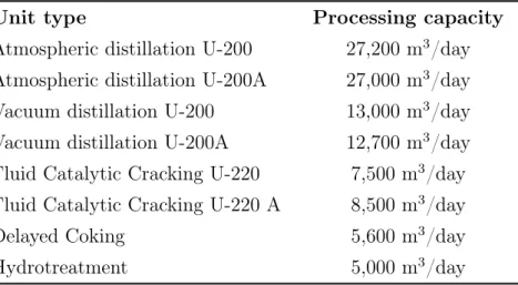
refinery is owned by PETROBRAS, and it is located in Paulínia (São Paulo). It has two distillation units, two vacuum units, two FCC units, and one delayed coking and catalytic hydrotreatment unit. Since the units of atmospheric distillation, vacuum distillation, and the two units of FCC are very similar, they were considered as one. As stated by Bueno (2003) this presumption greatly simplifies the model without losing precision. In Table 1 are shown the unit types in REPLAN and their processing capacities.
Table 1: Unit types and their processing capacities.
Unit type Processing capacity
Atmospheric distillation U-200 27,200 m3/day
Atmospheric distillation U-200A 27,000 m3/day
Vacuum distillation U-200 13,000 m3/day
Vacuum distillation U-200A 12,700 m3/day
Fluid Catalytic Cracking U-220 7,500 m3/day
Fluid Catalytic Cracking U-220 A 8,500 m3/day
Delayed Coking 5,600 m3/day
Hydrotreatment 5,000 m3/day
Source: Bueno (2003).
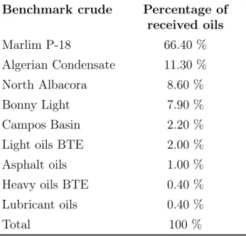
In Table 2 the percentage of different crude marks that is received on REPLAN is presented. For this model, only representative fractions were considered: Marlim P-18, Algerian Condensate, North Albacora, and Bonny Light.
15
Table 2: Benchmark crudes and their percentage received.
Benchmark crude Percentage of
received oils
Marlim P-18 66.40 % Algerian Condensate 11.30 % North Albacora 8.60 % Bonny Light 7.90 % Campos Basin 2.20 % Light oils BTE 2.00 % Asphalt oils 1.00 % Heavy oils BTE 0.40 % Lubricant oils 0.40 %
Total 100 %
Source: Bueno (2003).
units on HSC campaign (High Sulfur Content), which separates intermediates with high sulfur content; ASPHALT campaign, which separates heavy vacuum residuum for asphalt production; RATCRACK campaign, which separates atmospheric residuum and NORMAL campaign, which does not separate by any characteristic of the intermediate. Since no oils selected for this study have high sulfur content, and since asphalt production is not analyzed in this case study, both HSC and ASPHALT campaigns are not considered.
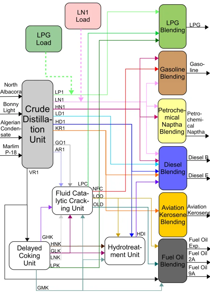
16 Chapter 4. Case Study
Figure 2: Model of REPLAN refinery.
Fluid
Cata-lytic
Crack-ing Unit
Crude
Distilla-tion
Unit
LPG
Blending
Gasoline
Blending
Petroche-mical
Naptha
Blending
Diesel
Blending
Aviation
Kerosene
Blending
Fuel Oil
Blending
LPG Algerian Conden-sate North Albacora Bonny Light Marlim P-18Hydrotreat-ment Unit
Delayed
Coking
Unit
LN1
Load
LPG
Load
LP1 LN1 HN1 LD1 HD1 KR1 GO1 AR1 VR1 LPC NFC LCO OLD HNK GLK LNK LPK GHK GMK HDI Gaso-line Petro- chemi-cal Naptha Diesel B Diesel E Aviation Kerosene Fuel Oil Exp. Fuel Oil 2A Fuel Oil 9A17
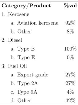
The selection of the products is based in the table of product types sold, presented in Table 3. Except for LPG, gasoline A, and petrochemical naphtha, which are the only representative product of their group, only representative products were chosen for the model, as aviation kerosene; diesel oil type B and type E, the last one by new market requirements; fuel oil export grade, fuel oil grade 2A and grade 9A representing low, medium and high viscosity oils, being selected by their composition, demand and quality difference. Coke is assumed to be burned for internal energy generation, thus it is not considered a product.
Table 3: Percentage of products sold by categories.
Category/Product %vol
1. Kerosene
a. Aviation kerosene 92%
b. Other 8%
2. Diesel
a. Type B 100%
b. Type E 0%
3. Fuel Oil
a. Export grade 27% b. Type 2A 27% c. Type 9A 4%
d. Other 42%
Source: Bueno (2003).
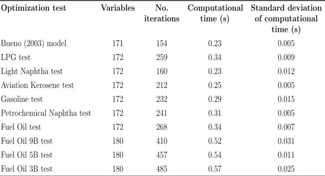
The model was solved in LINGO (Version 16), using the Global Solver. The solver reached the global optimum ($ 43,604/month) on every case studied, assuring precision on refinery planning results. The computational time required on each test was less than one second on an Intel i5-2410M processor, 8 GB RAM machine, using Windows 7. The small computational time assures the model usefulness into refinery planning, and is important for sensitivity analyses and the determination of break-even points of external loads and of new products.
18 Chapter 4. Case Study
hardware stress during solver’s execution. Since LINGO’s Global Solver is a deterministic method of solving nonlinear problems (GAU; SCHRAGE, 2004) and the results from the experiments showed variations of the computational time according to the stress on hardware, we concluded that these fluctuations are caused by computational issues (such as the concurrent use of cache memory by the simultaneous execution of other software).
As the number of iterations and the number of variables increases, the computational time also tends to increase, although not in a linear form because each test has its own peculiarities that influence the computational time required to solve through a specific method. For computational effort reasons, it is important to take note that all decision variables in the model are continuous.
Table 4: Computational time of global optimizations.
Optimization test Variables No.
iterations
Computational time (s)
Standard deviation of computational
time (s)
Bueno (2003) model 171 154 0.23 0.005
LPG test 172 259 0.34 0.009
Light Naphtha test 172 160 0.23 0.012
Aviation Kerosene test 172 212 0.25 0.005
Gasoline test 172 232 0.29 0.015
Petrochemical Naphtha test 172 241 0.31 0.005
Fuel Oil test 172 268 0.34 0.007
Fuel Oil 9B test 180 410 0.52 0.031
Fuel Oil 5B test 180 457 0.54 0.011
Fuel Oil 3B test 180 485 0.57 0.025
Source: Author.
Some external loads were studied to analyze if they are economically possible. Three intermediate loads were studied, as presented in Table 5: Light Naphtha, LPG, and Aviation Kerosene. Every load was introduced alone, with different volumes and proprieties. It is important to note that all obtained results related to the break-even point (BEP) and the sensitivity analysis refer to the REPLAN case study.
Light Naphtha
19
varies according to sulfur content, since sulfur content restrictions are very limited to products that use light naphtha, e.g. diesel.
LPG
The actual price of LPG is 127.8 dollars/m3. Since LPG is not reacted nor belongs to any other product nowhere in the refinery, the BEP equals to its acquisition price.
Kerosene
Kerosene shows a similar price to the same quantity of light naphtha, so we can infer that they are equivalent choices. This equivalency gives flexibility for the refinery.
Table 5: External loads behavior.
Stream
External volume added
(1000 m3
/month)
Sulfur content
Octane
rating BEP (dollars/ m 3
)
Light Naphtha 200 0.01% 90 152.0
Light Naphtha 100 0.01% 90 162.2
Light Naphtha 100 0.01% 120 162.2
Light Naphtha 100 0.01% 40 162.2
Light Naphtha 100 1.00% 90 140.0
LPG 100 0.00% – 127.8
Aviation Kerosene 100 0.09% – 162.4
Source: Author.
20 Chapter 4. Case Study
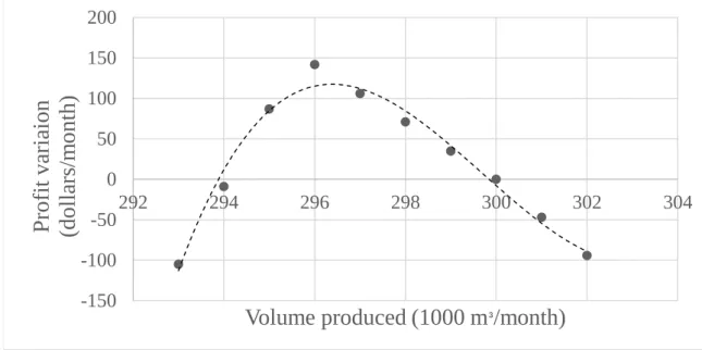
Figure 3: Sensitivity analysis for gasoline production. The dots represent the optimized profit variation for the simulated data. The dashed line is the tendency line. Source: Author.
-150 -100 -50 0 50 100 150 200
292 294 296 298 300 302 304
Pro
fi
t
v
ari
ai
o
n
(d
o
ll
ars
/m
o
n
th
)
Volume produced (1000 m
³/month)
Source: Author.
The profit variation versus the volume produced of petrochemical naphtha is presented in Figure 4. Through the linear pattern of petrochemical naphtha, we can infer that a reduction on its production would benefit REPLAN on every case. The additional profit would reach about 3,500 dollars/month for the total cease of production case. This graph shows to the planner that petrochemical naphtha production should be avoided at REPLAN.
Figure 4: Sensitivity analysis for petrochemical naphtha production. The dots represent the optimized profit variation for the simulated data. The dashed line is the tendency line.
-500 0 500 1000 1500 2000 2500 3000 3500 4000
0 10 20 30 40 50 60 70 80 90 100 110
Pro
fi
t
v
ari
at
io
n
(d
o
ll
ar
s/
m
o
n
th)
21
The profit variation versus the volume produced of fuel oil export grade is presented in Figure 5. There is a local optimum that reaches 1,650 dollars/month. However, there is a wide range of production available to increase profit. The slope is steeper than on gasoline analysis: a reduction of a mere 5,000 m3/month increases refinery profit by approximately 670 dollars/month. The planner must pay attention to this behavior, since a small variation could directly influence the profit.
Figure 5: Sensitivity analysis for fuel oil export production. The dots represent the optimized profit variation for the simulated data. The dashed line is the tendency line.
-500 0 500 1000 1500 2000
90 110 130 150 170
Profi
t
va
ri
at
io
n
(d
o
ll
ars
/m
o
n
th
)
Volume produced (1000 m
³/month)
Source: Author.
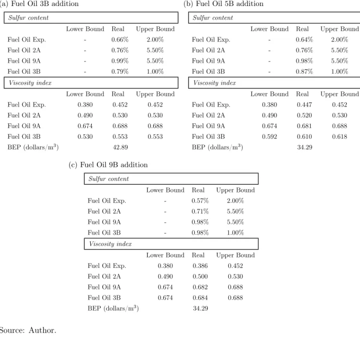
In the literature, there is a lack of detailed economic analysis about product adding. In this study, we propose a method for quickly evaluating the economical availability of adding a new product in the planning. After the addition of the new product in the model, the BEP was determined to analyze the impact caused by the product in the refinery.
Brazilian laws recognize 18 variations of fuel oil, which are classified based on viscosity and sulfur content. The well-defined and continuous ranges of viscosity for fuel oils made this type of product a suitable option for analysis. The products chosen were fuel oil grade 3B, 5B, and 9B. They have low sulfur content (1.00% maximum) and present low, medium, and high viscosity, respectively. The model was run several times, producing a batch of 100,000 m3/month for each new product separately, varying the new product price until the profit matched the original one. This way we found the BEP. The results of the addition of each product are presented in Table 6.
22 Chapter 4. Case Study
Table 6: New product addition.
(a) Fuel Oil 3B addition
Sulfur content
Lower Bound Real Upper Bound Fuel Oil Exp. - 0.66% 2.00% Fuel Oil 2A - 0.76% 5.50% Fuel Oil 9A - 0.99% 5.50% Fuel Oil 3B - 0.79% 1.00%
Viscosity index
Lower Bound Real Upper Bound Fuel Oil Exp. 0.380 0.452 0.452 Fuel Oil 2A 0.490 0.530 0.530 Fuel Oil 9A 0.674 0.688 0.688 Fuel Oil 3B 0.530 0.553 0.553 BEP (dollars/m3) 42.89
(b) Fuel Oil 5B addition
Sulfur content
Lower Bound Real Upper Bound Fuel Oil Exp. - 0.64% 2.00% Fuel Oil 2A - 0.76% 5.50% Fuel Oil 9A - 0.98% 5.50% Fuel Oil 3B - 0.87% 1.00%
Viscosity index
Lower Bound Real Upper Bound Fuel Oil Exp. 0.380 0.447 0.452 Fuel Oil 2A 0.490 0.520 0.530 Fuel Oil 9A 0.674 0.681 0.688 Fuel Oil 3B 0.592 0.610 0.618 BEP (dollars/m3) 34.29
(c) Fuel Oil 9B addition
Sulfur content
Lower Bound Real Upper Bound Fuel Oil Exp. - 0.57% 2.00% Fuel Oil 2A - 0.71% 5.50% Fuel Oil 9A - 0.98% 5.50% Fuel Oil 3B - 0.98% 1.00%
Viscosity index
Lower Bound Real Upper Bound Fuel Oil Exp. 0.380 0.386 0.452 Fuel Oil 2A 0.490 0.500 0.530 Fuel Oil 9A 0.674 0.682 0.688 Fuel Oil 3B 0.674 0.684 0.688 BEP (dollars/m3) 34.29
Source: Author.
Chapter
5
Conclusions
A global optimum in the blending operations was reached in every case studied using LINGO optimization solver, assuring precise results on refinery planning. The model presented a quick solution time in every test performed, which is very important for sensitivity analyses that can be used by planners for studying refinery’s profit behavior.
The sensibility analyses showed that any variation on the produced volumes of gasoline at REPLAN can strongly influence its profit, and the production of petrochemical naphtha is bad at any volume produced. Other products as fuel oil export grade give flexibility to REPLAN, as they weakly influence REPLAN’s profit. This type of analysis can show capacity bottlenecks or undesirable products for any refinery and any product, enabling the planners to look for unseen potential improvements and problems.
Another contribution of this work was the modeling of the external loads transfer to the refinery. The addition of intermediate loads does not interfere deeply with the refinery scheme, so it adds flexibility, an important characteristic for keeping up on the unstable market of the petroleum industry. The BEP was obtained for several intermediates that could be transferred into REPLAN, thus allowing a more detailed planning of the refinery and an increase of its profitability. Adjusting the proposed model, it is possible to analyze the acquisition of external loads for other refineries.
The properties of the external loads influence its BEP differently, as seen on REPLAN study case: the light naphtha’s BEP is influenced by the sulfur content, while the octane rating influences a lot less. It is also possible to determine equivalent products through the BEP: at REPLAN, light naphtha and kerosene are equivalent acquisitions since their BEP is the same.
24 Chapter 5. Conclusions
profitable without disrupting the refinery scheme, since only the blending pools are modified. Sensitivity analyses obtained the BEP of several new products that could be produced at REPLAN and showed how the other products would be affected. By determining the BEP, it is possible to evaluate the profitability of the new product.
Bibliography
ALATTAS, A. M.; GROSSMANN, I. E.; PALOU-RIVERA, I. Integration of nonlinear crude distillation unit models in refinery planning optimization. Industrial and Engineering Chemistry Research, v. 50, n. 11, p. 6860–6870, 2011. ISSN 08885885.
BODINGTON, C. E.; BAKER, T. E. A History of Mathematical Programming in the Petroleum Industry. Interfaces, v. 20, n. 4, p. 117–127, 1990. ISSN 00922102.
BUENO, C. Planejamento operacional de refinarias. 110 p. Thesis — Universidade
Federal de Santa Catarina, Florianópolis, 2003.
GAU, C.-Y.; SCHRAGE, L. E. Implementation and Testing of a Branch-and-Bound Based Method for Deterministic Global Optimization: Operations Research Applications. In: FLOUDAS, C.; PARDALOS, P. (Ed.). Frontiers in global optimization. [S.l.]: Springer US, 2004. p. 145–164. ISBN 9781461379614.
GUEDDAR, T.; DUA, V. Disaggregation—aggregation based model reduction for refinery-wide optimization.Computers & Chemical Engineering, v. 35, n. 9, p. 1838–1856,
sep 2011. ISSN 00981354.
JOLY, M. Refinery production planning and scheduling: The refining core business.
Brazilian Journal of Chemical Engineering, v. 29, n. 2, p. 371–384, 2012. ISSN 01046632.
KOO, L. Y.; ADHITYA, A.; SRINIVASAN, R.; KARIMI, I. Decision support for integrated refinery supply chains. Computers & Chemical Engineering, v. 32, n. 11, p. 2787–2800, nov 2008. ISSN 00981354.
LÁNG, P.; SZALMÁS, G.; CHIKÁNY, G.; KEMÉNY, S. Modelling of a crude distillation column. Computers & Chemical Engineering, v. 15, n. 2, p. 133–139, feb
1991. ISSN 00981354.
LI, C.; HE, X.; CHEN, B.; CHEN, B.; GONG, Z.; QUAN, L. Integrative optimization of refining and petrochemical plants. In: 16th European Symposium on Computer Aided Process Engineering and 9th International Symposium on Process Systems Engineering. [S.l.]: Elsevier, 2006. (Computer Aided Chemical Engineering, v. 21), p. 2039–2044. ISBN 9780444529695. ISSN 15707946.
Bibliography
MENEZES, B. C.; KELLY, J. D.; GROSSMANN, I. E. Improved Swing-Cut Modeling for Planning and Scheduling of Oil-Refinery Distillation Units. Industrial & Engineering Chemistry Research, American Chemical Society, v. 52, n. 51, p. 18324–18333, dec 2013.
ISSN 08885885.
MORE, R. K.; BULASARA, V. K.; UPPALURI, R.; BANJARA, V. R. Optimization of crude distillation system using aspen plus: Effect of binary feed selection on grass-root design. Chemical Engineering Research and Design, v. 88, n. 2, p. 121–134, feb 2010.
ISSN 02638762.
MORO, L. F. Process technology in the petroleum refining industry—current situation and future trends.Computers & Chemical Engineering, v. 27, n. 8-9, p. 1303–1305, sep
2003. ISSN 00981354.
MORO, L. F. L.; PINTO, J. M. Mixed-Integer Programming Approach for Short-Term Crude Oil Scheduling. Industrial & Engineering Chemistry Research, v. 43, n. 1, p.
85–94, 2004. ISSN 08885885.
PINTO, J.; JOLY, M.; MORO, L. Planning and scheduling models for refinery operations. Computers & Chemical Engineering, v. 24, n. 9-10, p. 2259–2276, oct 2000. ISSN 00981354.
PINTO, J. M.; MORO, L. F. L. A planning model for petroleum refineries. Brazilian Journal of Chemical Engineering, v. 17, n. 4, p. 575–585, 2000. ISSN 01046632.
PITTY, S. S.; LI, W.; ADHITYA, A.; SRINIVASAN, R.; KARIMI, I. Decision support for integrated refinery supply chains. Computers & Chemical Engineering, v. 32, n. 11,
p. 2767–2786, nov 2008. ISSN 00981354.
SHOBRYS, D. E.; WHITE, D. C. Planning, scheduling and control systems: why cannot they work together. Computers & Chemical Engineering, v. 26, n. 2, p. 149–160, feb