Carlos Henrique Marchi
Senior Member, ABCM
[email protected] Federal University of Parana - UFPR Department of Mechanical Engineering P. O. Box 19040 81531-980 Curitiba, PR. Brazil
Maykel Alexandre Hobmeir
Numerical Solution of Staggered
Circular Tubes in Two-Dimensional
Laminar Forced Convection
This paper aims to demonstrate the importance of adequately estimating the discretization error intrinsic in the result of any numerical simulation. The problem under consideration is forced convection in a staggered circular tube heat exchanger. The problem is solved to analyze the effect of the distance between the tubes, aiming to optimize the heat exchanger’s geometrical configuration by two Reynolds numbers (50 and 100). The present work did not confirm the existence of an optimal geometrical point for the operation of staggered circular tube heat exchangers, as claimed in a numerical study published in the literature.
Keywords: finite volume, CFD, numerical error, GCI, CFX
Introduction
Today, the reports available in the literature on estimates of discretization errors in the results of numerical simulations can be classified into four categories: (1) No estimate is made and the numerical solution is obtained on a single grid; (2) no estimate is made but numerical solutions obtained on two or more grids are presented, usually with graphic comparisons of profiles of field variables on the various grids; (3) estimates are made but are based on error estimators that are little reliable or inadequate, such as the delta estimator (Demirdzic, Lilek and Peric, 1992); and (4) estimates are made based on the state of the art, i.e., using the best error estimators available, such as the GCI (Grid Convergence Index) estimator (Roache, 1994).1
Based on a case study, this work aims to demonstrate the importance of adequately estimating the discretization error involved in the result of a simulation, particularly when the purpose is to optimize a system’s operation. The problem under consideration is the geometric optimization of the forced heat convection in a bank of circular tubes with fixed volume restriction of the heat exchanger.
The two main goals in computational fluid dynamics are to obtain numerical solutions that are accurate and reliable (Shyy et al., 2002), both of which depend on the estimate of the numerical error. The acceptable magnitude of the numerical error depends, among other factors, on the purpose of the numerical solution, the financial resources involved, the time allowed or available to carry out the simulations, and the existing computational resources. Aware that numerical solutions contain errors, it is important to estimate them because, among other reasons, when the error is greater than acceptable, it compromises the reliability of the use of the numerical solution.
The methods employed in the solution of an engineering problem can be divided into three types: experimental, analytical and numerical (Tannehill, Anderson and Pletcher, 1997). Figure 1 illustrates the types of errors involved in these methods, i.e., experimental, modeling and numerical errors. The experimental error is the difference between the true value of a variable of interest and its experimental result (ISO, 1993). The true value is usually unknown, so one can only estimate the value of the experimental error. This estimated value is called uncertainty, and the process whereby it is quantified is known as uncertainty analysis. Methods for quantifying the uncertainty of experimental results are given in
Paper accepted February, 2006. Technical Editor: Aristeu da Silveira Neto.
ISO (1993), Coleman and Steele (1999) and Holman (1994), for example.
The modeling error is the difference between the true value of a variable of interest and its analytical solution (Ferziger and Peric, 1999). Again, the true value is usually unknown; therefore, one can only estimate the value of the modeling error [Umod(Qnum)]. This is
done by comparing the analytical and numerical solutions (Qnum)
against experimental results (Qexp):
num
num Q Q
Q
Umod( ) = exp − (1)
Modeling errors are caused by simplifications of the real phenomenon in the conception of mathematical models. The process that quantifies this type of error has recently been called validation (Roache, 1998; AIAA, 1998). The purpose of validation is to determine to what extent a mathematical model represents a given real phenomenon. The process of validation is dealt with, for instance, by Roache (1998), Stern et al. (2001) and Aeschliman and Oberkampf (1998).
The numerical error of a variable of interest is the difference between its exact analytical solution and its numerical solution (Ferziger and Peric, 1999). Therefore, the ideal numerical solution is equal to the exact analytical solution of the problem, i.e., it is the solution in which the numerical error is null. Examples of variables of interest in fluid dynamics are: velocity, temperature, pressure, density, mass flow rate, heat transfer rate and force. The process whereby the numerical error is quantified has recently been given the name of verification (Roache, 1998; AIAA, 1998). The objective of verification is to determine to what extent a mathematical model is solved adequately through a numerical method.
The value of the true numerical error is independent of experimental results but can only be obtained when the analytical solution of the mathematical model is known. However, in practical terms, i.e., for numerical solutions of mathematical models whose analytical solution is unknown, the numerical error cannot be obtained. In such cases, the value of the analytical solution must be estimated. Thus, instead of the true numerical error, one calculates the estimated numerical error [Unum(Qnum)], which is evaluated by
the difference between the estimated analytical solution (Q∞) and
the numerical solution (Qnum), in other words:
num num
num Q Q Q
U ( ) = ∞ − (2)
1) Discretization error: originates from numerical
approximations used in discretizing a mathematical model (Tannehill, Anderson and Pletcher, 1997; Ferziger and Peric, 1999; Roache, 1998). This error is usually reduced by decreasing the size of the grid’s elements, i.e., by reducing the distance between two consecutive nodes in the grid. 2) Iteration error: is the difference between the exact solution
of the discretized equations and the numerical solution in a given iteration (Ferziger and Peric, 1999). Generally speaking, iteration errors decrease as the number of iterations increases.
3) Round-off error: occurs mainly due to the finite representation of real numbers in computations. It increases as the size of the grid’s elements decreases, i.e., with increasing numbers of nodes, elements or volumes in the grid.
4) Programming error: includes human errors in the implementation and use of a computational program.
The following will be presented in subsequent sections: the definition of the physical problem under consideration and its corresponding mathematical model; numerical results of Matos et al. (2001) and of this work; the estimate of discretization errors based on Roache’s (1994) GCI estimator; the estimate of the modeling errors; and the conclusion of this work.
Nomenclature
cp = specific heat at constant pressure
D = tube diameter
Fs = safety factor of the GCI estimator k = thermal conductivity
L, H, W = size of the heat exchanger in the x, y and z directions N = number of elements of the grid
p = pressure
pL = asymptotic order of the discretization error
Pr = Prandtl number
q = total heat transfer rate of the heat exchanger
Q = dimensionless overall thermal conductance of the heat exchanger
Qexp = experimental result
Qnum = numerical solution Q∞ = estimated analytical solution
r = ratio of refinement between the fine and coarse grids Re = Reynolds number
S = spacing between the tubes T = temperature
Tw = temperature on the tube walls T∞ = free stream temperature
u, v = components of the velocity vector in the x and y directions Umod = modeling error
Unum = estimated numerical error
U∞ = free stream velocity
x, y = spatial coordinates Greek Symbols ρ = density µ = viscosity Subscripts
1 fine grid
2 coarse grid
Definition of the Problem
Forced convection in a heat exchanger consisting of a set of circular tubes was studied by Stanescu, Fowler and Bejan (1996).
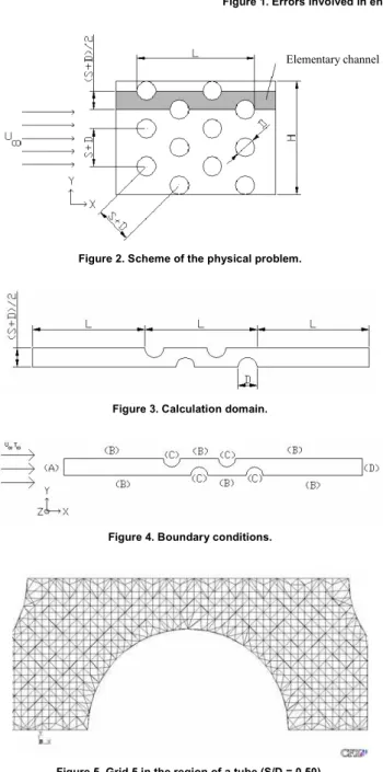
Figure 2 shows a scheme of the physical problem. In this figure, D = tube diameter; S = spacing between the tubes, whose centers lie at the vertices of an equilateral triangle; U∞ = free stream velocity; L
and H = size of the heat exchanger in the x and y directions, respectively. The tubes are staggered. Their longitudinal axes are perpendicular to the flow of the coolant (air). The fluid (water) to be cooled flows through the circulating tubes.
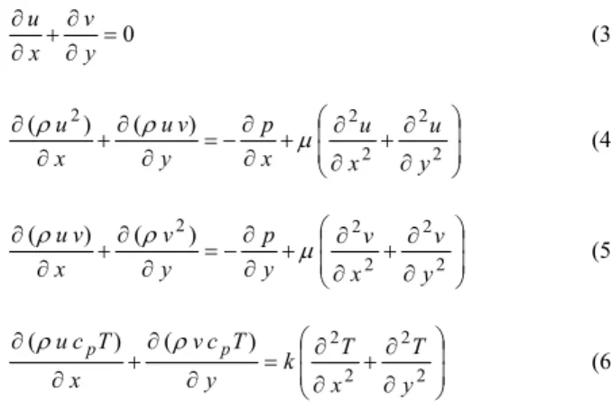
This problem can be modeled mathematically by equations of mass, momentum and energy conservation (Tannehill, Anderson and Pletcher, 1997):
0 = ∂ ∂ + ∂ ∂ y v x u (3) ∂ ∂ + ∂ ∂ + ∂ ∂ − = ∂ ∂ + ∂ ∂ 2 2 2 2 2 ) ( ) ( y u x u x p y v u x u µ ρ ρ (4) ∂ ∂ + ∂ ∂ + ∂ ∂ − = ∂ ∂ + ∂ ∂ 2 2 2 2 2 ) ( ) ( y v x v y p y v x v u µ ρ ρ (5) ∂ ∂ + ∂ ∂ = ∂ ∂ + ∂ ∂ 2 2 2 2 ) ( ) ( y T x T k y T c v x T c
u p ρ p
ρ
(6)
where x and y = spatial coordinates, T = temperature, u and v = components of the vector velocity in the x and y directions, ρ = density, p = pressure, µ = viscosity, k = thermal conductivity, and cp
= specific heat at constant pressure. This mathematical model can be obtained, considering: Newtonian and incompressible fluid; steady two-dimensional laminar flow; zero viscous dissipation; and constant properties.
The heat exchanger consists of the 12 tubes depicted in Figure 2. Due to the symmetry of the problem, whose elementary channel (see Fig. 2) is repeated, the calculation domain considered here is shown in Fig. 3. The reason for using an L length before and after the tubes is discussed in the work of Stanescu, Fowler and Bejan (1996) and Matos et al. (2001). The boundary conditions indicated in Fig. 4 are:
∞
∞ = =
=U v T T
u , 0,
) A
( (7)
0 , 0 , 0 ) B ( = ∂ ∂ = = ∂ ∂ y T v y u (8) w T T v
u=0, =0, =
) C
( (9)
0 , 0 , 0 ) D ( = ∂ ∂ = ∂ ∂ = ∂ ∂ x T x v x u (10)
where T∞ = free stream temperature, and Tw = temperature on the
tube walls.
The variable of interest of the problem is the dimensionless overall thermal conductance (Q) of the heat exchanger, defined in Stanescu, Fowler and Bejan (1996) and Matos et al. (2001) as:
) ( 2 ∞ − = T T kLHW qD Q w (11)
Figure 1. Errors involved in engineering problem solving methods.
Elementary channel
Figure 2. Scheme of the physical problem.
Figure 3. Calculation domain.
Figure 4. Boundary conditions.
Figure 5. Grid 5 in the region of a tube (S/D = 0.50).
Numerical Results
Results of Matos et al. (2001)
Matos et al. (2001) solved the problem by employing an altered version of the FEAP (Finite Element Analysis Program) code originally written by Zienkiewicz and Taylor (1989) and using the finite element method. The advective terms of the mathematical model were discretized with an upwind scheme (Hughes, 1978). Details of the numerical methodology are given in the work of Matos et al. (2001).
Their study aimed to determine the heat exchanger’s optimal spacing (S), i.e., the value of S that would result in the maximum Q for each Reynolds number (Re), keeping the heat exchanger’s 12 tubes and volume (LHW) fixed. For circular tubes, numerical results were obtained for an S/D of 0.1 to 1.25 and an Re of 50 to 775, where
µ
ρU∞D =
Re (12)
In addition, numerical results were obtained for elliptical tubes with several eccentricities, S/D and Re. Tables 1 and 2 present some of the numerical results (with 5,180 elements) of Matos et al. (2001) for circular tubes, as well as the grids utilized. Table 1 indicates that the maximum value of Q is 3.55 in S/D = 1.0 for Re = 50, and Q is 5.71 in S/D = 0.5 for Re = 100.
The discretization error of the numerical solution for Q was evaluated through the relative delta estimator defined by (Demirdzic, Lilek and Peric, 1992)
1 2 1 1) (
Q Q Q Q
Unum
−
= ∆
(13)
where subindices 1 and 2 refer to Table 2, indicating fine and coarse grids, respectively. According to Matos et al. (2001), the maximum discretization error estimated for the numerical solutions in Table 1, calculated with Eq. (13), is 1%.
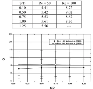
Table 1. Some of the results for Q of Matos et al. (2001).
S/D Re = 50 Re = 100
Table 2. Grids used by Matos et al. (2001).
Grid N = Number of elements 1 5,380 2 5,180 3 2,508
Results of this Work
In this work, the problem was solved with version 5.6 of the CFX computational code (CFX, 2003), which uses the finite volume method on nonstructured grids; coupled solution of mass and momentum; algebraic multigrid; incomplete upper-lower factorization (ILU) smoother; and implicit, pressure-based algorithm for all flow speeds. The advective terms of the mathematical model were discretized with two schemes (Ferziger and Peric, 1999): UDS (Upstream Differencing Scheme) and CDS (Central Differencing Scheme), which are, respectively, schemes of 1st- and 2nd-order accuracy.
The data used in the simulations were: D = 6.35 mm; L = 39.2 mm; H = 35.2 mm; W = 134 mm; T∞ = 298.15 K; Tw = 310.85 K; µ
= 184.6x10⁻⁷ N.s/m2; c
p = 1007 J/kg.K; ρ = 1.1614 kg/m3; Pr = 0.72; k = 26.3x10⁻³ W/m.K; U
∞ = 0.125 m/s for Re = 50; U∞ = 0.250 m/s
for Re = 100; where Pr is Prandtl number.
Tables 3 and 4 list the numerical results of this work and the grids utilized. Figure 5 shows grid 5 in the region of a tube for S/D = 0.50.
Table 3. Results of this work for Q obtained with the finest grid of Table 4.
S/D Re = 50 (UDS) Re = 50 (CDS) Re = 100 (UDS)
0.50 4.29 4.15 7.70
0.75 4.52 4.30 7.75
1.00 4.75 4.37 8.10
Table 4. Number of elements (N) of the grids used in this work.
Grid S/D = 0.50 S/D = 0.75 S/D = 1.00
1 98,679 100,318 49,926
2 49,870 51,200 24,624
3 25,060 24,720 12,359
4 12,085 12,534 6,396
5 6,138 6,224 ---
Considering the various grids, UDS and CDS, the two Reynolds numbers and the three S/D values used, 42 numerical simulations were carried out in this work. In each of these simulations, the convergence criterion employed was the drop by 8 orders of magnitude of the nondimensionalized residue for each of the four differential equations involved in the solution. Double precision was used in all the simulations. With the CDS scheme, the average computation time was 22 min and 24 h 30 min, respectively, for the coarser and finer grids. In the case of the UDS scheme, the average computation time was approximately half that of the CDS scheme. The simulations were performed using a microcomputer with an AMD ATHLON XP 2100+ processor and 512 MB of RAM.
Estimate of Discretization Errors
From its numerous citations and widespread use, and according to the experience of one of the authors of this work, Roache’s GCI (Roache, 1994) can be considered the most reliable of the current estimators of discretization errors. According to the GCI, the estimate of the discretization error of the numerical solution obtained on a fine grid (Q1) is:
) 1 ( )
( 1 1 2
− −
=
L p s GCI
num
r Q Q F Q
U (14)
where Fs is a safety factor of 3 for general applications; pL is the
asymptotic order of the discretization error; subindices 1 and 2 refer to Tables 2 and 4; and r is the ratio of refinement between the fine and coarse grids, which, for two-dimensional nonstructured grids, is calculated by (Roache, 1994):
2 1
N N
r = (15)
where N1 and N2 represent, respectively, the number of elements of
the fine and coarse grids. The GCI supplies even more reliable error estimates when used with the apparent order (pU) (Marchi and Silva,
2002).
Estimate of Discretization Errors for the Results of Matos et al. (2001)
Considering the maximum discretization error estimated for the numerical solutions of Table 1, of 1%, pL = 1, Fs = 3 and r = 1.019
for grids 1 and 2 of Table 2, one can deduce from Eqs. (13) and (14) that
1 1) 1.58
(Q Q
UnumGCI = (16)
Hence, with Eq. (16) and the results of Table 1, it is possible to obtain more reliable estimates for the discretization errors of the numerical solutions of Matos et al. (2001), as shown in Table 5 and Fig. 6. According to Eq. (13), the delta estimator’s 1% error estimate made by Matos et al. (2001) is transformed into 158% with the GCI estimator, Eq. (16). The same scales are used in Fig. 6 to 10 to allow for a visual qualitative comparison of the various numerical and experimental results and their respective error estimates.
Table 5. Estimated discretization error for Q of the results of Matos et al. (2001).
S/D Re = 50 Re = 100
0.10 4.41 8.72 0.50 5.42 9.02 0.75 5.53 8.67 1.00 5.61 8.36
1.25 5.56 ---
0,00 0,25 0,50 0,75 1,00 1,25
-5 0 5 10 15 20 25
Re = 50, Matos et al. (2001) Re = 100, Matos et al. (2001)
Q
S/D
The two main problems of the delta estimator, Eq. (13), used by Matos et al. (2001) are: (i) it does not consider the order of the discretization error, i.e., the asymptotic (pL) or apparent (pU) order;
and (ii) it does not consider the grid refinement ratio (r) which allows the error estimate to become arbitrarily small when one uses r→ 1.
The results of Matos et al. (2001) listed in Table 1 indicate that the optimal point of the heat exchanger, i.e., the maximum value of Q, is 3.55 in S/D = 1.0 for Re = 50. In the interval of S/D = 0.1 to 1.25, the variation of Q was 2.79 to 3.55, i.e., 0.76. But Table 5 shows that that estimate of the discretization error varies from 4.41 to 5.61 for Re = 50. Therefore, it is to be expected that the discretization error is far greater than the effect of the geometric optimization (S/D) of the heat exchanger. The situation is even worse for Re = 100. The maximum value of Q is 5.71 in S/D = 0.50. In the interval of S/D = 0.1 to 1.0, the variation of Q was 5.29 to 5.71, i.e., 0.42. However, Table 5 indicates that the estimate of the discretization error varies from 8.36 to 9.02, as graphically illustrated in Fig. 6. With the level of discretization error involved in the solutions of Matos et al. (2001), it is impossible to reliably evaluate the heat exchanger’s geometric optimization (S/D) or the effect of the Reynolds number (Re).
Estimate of Discretization Errors for the Results of this Work
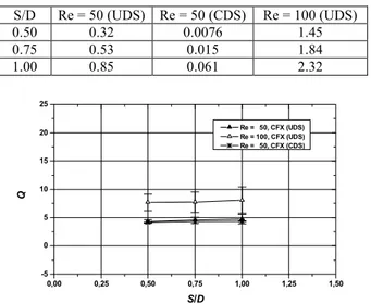
The discretization errors of this work’s numerical solutions, shown in Table 6 and Fig. 7, can be estimated based on Eqs. (14) and (15), Fs = 3 and the data of Table 4. pL = 1 and 2 were
considered, respectively, for the numerical solutions obtained with the UDS and CDS schemes. In each case, the grid refinement ratio (r) was about 1.4. As can be seen, (i) the level of estimated discretization errors is inferior to the effect of the variation of the Reynolds number (Re) of 50 to 100; and (ii) within the estimated margins of error, the numerical solutions obtained with schemes UDS and CDS are coherent for Re = 50, i.e., the margin of error of UDS involves that of CDS.
Table . Estimated discretization error for Q of the results of this work.
S/D Re = 50 (UDS) Re = 50 (CDS) Re = 100 (UDS)
0.50 0.32 0.0076 1.45
0.75 0.53 0.015 1.84
1.00 0.85 0.061 2.32
0,00 0,25 0,50 0,75 1,00 1,25 1,50
-5 0 5 10 15 20 25
Re = 50, CFX (UDS) Re = 100, CFX (UDS) Re = 50, CFX (CDS)
Q
S/D
Figure 7. Results for Q of this work and estimate of their errors.
With Tables 3 and 6, one can see that the geometric effect (S/D) causes Q to vary 0.46 and 0.22, respectively, for the numerical solutions obtained with the UDS and CDS schemes for Re = 50, while the maximum estimated discretization error is 0.85 (UDS) and
0.061 (CDS). For Re = 100, the geometric effect (S/D) causes Q to vary 0.40 for the numerical solutions obtained with the UDS scheme, and the maximum estimated discretization error is 2.32. Only the numerical solutions obtained with the CDS scheme allow for the real geometric optimization of the heat exchanger, since the level of estimated discretization error is inferior to the geometric effect.
Calculation of Modeling Errors
An empirical correlation of the problem under consideration in this study can be found in Bejan (1993) for Nusselt number. Based on this correlation, one can obtain the heat transfer rate and, finally, Q with Eq. (11) for the data used in this work. The experimental results are given in Table 7 and Fig. 8 with the experimental uncertainty, which is ±15%.
Table 7. Experimental results for Q obtained based on Bejan (1993).
S/D Re = 50 Re = 100
0.10 15.26 21.19 0.50 7.07 9.33 0.75 6.40 8.44 1.00 6.01 7.93 1.25 5.76 7.61
0,00 0,25 0,50 0,75 1,00 1,25
-5 0 5 10 15 20 25
Re = 50, Bejan (1993) Re = 100, Bejan (1993)
Q
S/D
Figure 8. Experimental (Bejan, 1993) results for Q and their uncertainties.
The estimated modeling errors for Q of the results of Matos et al. (2001) and calculated from Eq. (1) is shown in Table 8. Figure 9 presents the experimental results for Q obtained based on Bejan (1993), and Matos et al.’s (2001) numerical results, as well as their respective experimental uncertainty and estimated discretization error. The estimated modeling errors for Matos et al.’s (2001) numerical results vary from 2.24 to 12.47 for Re = 50, while the geometric effect (S/D) causes Q to vary 0.76. For Re = 100, the estimated modeling errors vary from 2.64 to 15.67 and the geometric effect (S/D) causes Q to vary 0.42. Moreover, the qualitative behavior of the numerical and experimental results differs. The experimental results tending to decrease monotonically as S/D increases, while the numerical results display a maximum within the S/D interval considered. With the level of the modeling error involved in the numerical solution of Matos et al. (2001), one cannot reliably evaluate the geometric optimization (S/D) of the heat exchanger.
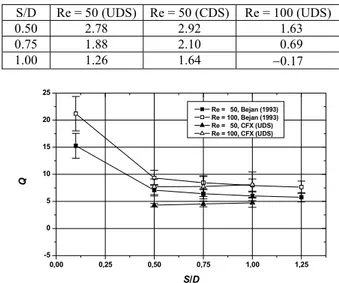
work vary from 1.26 to 2.78 for Re = 50, while the geometric effect (S/D) causes Q to vary 0.46. The estimated modeling errors for Re = 100 vary from -0.17 to 1.63 and the geometric effect (S/D) causes Q to vary 0.40. With the level of modeling errors involved in the numerical solutions of this work, the heat exchanger’s geometric optimization (S/D) can also not be evaluated reliably.
Table 8. Estimated modeling error for Q of the results of Matos et al. (2001).
S/D Re = 50 Re = 100
0.10 12.47 15.67 0.50 3.64 3.62 0.75 2.90 2.95 1.00 2.46 2.64
1.25 2.24 ---
0,00 0,25 0,50 0,75 1,00 1,25
-5 0 5 10 15 20 25
Re = 50, Bejan (1993) Re = 100, Bejan (1993) Re = 50, Matos et al. (2001) Re = 100, Matos et al. (2001)
Q
S/D
Figure 9. Experimental (Bejan, 1993) and numerical (Matos et al., 2001) results for Q.
For the numerical solutions of Matos et al. (2001) in the S/D interval of 0.5 to 1, the maximum values of estimated discretization error are 5.61 and 9.02, respectively, for Re = 50 and 100. In contrast, the results of this work are 0.85 (UDS, Re=50), 0.061 (CDS, Re=50) and 2.32 (UDS, Re=100). Hence, the estimated discretization errors of this work are substantially inferior to those of Mattos et al. (2001), as expected in view of the much more refined grids used in this study.
For Matos et al.’s (2001) numerical solutions in the S/D interval of 0.5 to 1, the maximum values of estimated modeling error are 3.64 and 3.62, respectively, for Re = 50 and 100. The results of this study, on the other hand, are 2.92 (Re=50) and 1.63 (Re=100), indicating that the modeling errors of this work are slightly inferior to those of Mattos et al. (2001), but of the same order and significantly greater than the geometric effect. Therefore, it was not possible to verify the existence of an optimal geometric point (S/D) for the heat exchanger, as claimed by Matos et al. (2001), either from the purely theoretical standpoint (numerical errors) or from that of the real problem (modeling errors). This conclusion is valid for situations in which the heat exchanger’s volume (LWH) and number of tubes (12) are fixed, while the distance between the tubes is variable. There is a similar problem, in which the heat exchanger’s volume is fixed while the number of tubes and the distance between them is variable. There are experimental results (Stanescu, Fowler and Bejan, 1996) for this other problem that show the existence of an optimal geometric point.
Table 9. Estimated modeling error for Q of the results of this work.
S/D Re = 50 (UDS) Re = 50 (CDS) Re = 100 (UDS)
0.50 2.78 2.92 1.63
0.75 1.88 2.10 0.69
1.00 1.26 1.64 −0.17
0,00 0,25 0,50 0,75 1,00 1,25
-5 0 5 10 15 20 25
Re = 50, Bejan (1993) Re = 100, Bejan (1993) Re = 50, CFX (UDS) Re = 100, CFX (UDS)
Q
S/D
Figure 10. Experimental (Bejan, 1993) and numerical (this work) results for Q.
Conclusion
The delta estimator, Eq. (13), should not be used to estimate discretization errors of numerical solutions. Instead, for the same purpose, we recommend the use of the GCI estimator (Roache, 1994), Eq. (14).
Based on numerical solutions, Matos et al. (2001) showed that there is an optimal geometric point for the operation of staggered circular tube heat exchangers, for situations in which the heat exchanger’s volume (LWH) and number of tubes (12) are fixed and the distance between the tubes is variable. This geometric effect is related with the distance between the tubes. However, the real existence of this optimal point is doubtful, because:
1) The qualitative behavior of the numerical and experimental results differs.
2) The level of the discretization error estimated for the numerical solutions of Matos et al. (2001) is one order of magnitude greater than the geometric effect, for grids containing approximately 5 thousand elements.
3) The level of the discretization error estimated for the numerical solutions of this work is in the order (UDS) of magnitude of the geometric effect or even lower (CDS) for grids containing approximately 100 thousand elements.
4) Even so, the levels of modeling error estimated for the numerical solutions of Matos et al. (2001) and of this study are greater than the geometric effect.
Acknowledgements
References
Aeschliman, D. P., and Oberkampf, W. L., 1998, “Experimental Methodology for Computational Fluid Dynamics Code Validation”, AIAA Journal, Vol. 36, pp. 733-741.
AIAA, 1998, “Guide for the Verification and Validation of Computational Fluid Dynamics Simulations”, AIAA G-077-1998, American Institute of Aeronautics and Astronautics, Reston.
Bejan, A., 1993, “Heat Transfer”, pp. 270-272, Wiley, New York. CFX Ltd., 2003, “CFX-5 Reference Guide”, Didcot Oxfordshire, United Kingdom.
Coleman, H. W., and Steele, W. G., 1999, “Experimentation and Uncertainty Analysis for Engineers”, 2nd ed., Wiley, New York.
Demirdzic, I., Lilek, Z., and Peric, M., 1992, “Fluid Flow and Heat Transfer Test Problems for Non-Orthogonal Grids: Bench-mark Solutions”, International Journal for Numerical Methods in Fluids, Vol. 15, pp. 329-354.
Ferziger, J. H., and Peric, M., 1999, “Computational Methods for Fluid Dynamics”, 2nd ed., Springer-Verlag, Berlin, 389 p.
Holman, J. P., 1994, “Experimental Methods for Engineers”, 6th ed., McGraw-Hill, New York.
Hughes, T. J. R., 1978, “A Simple Scheme for Developing Upwind Finite Elements”, Int. Journal for Numerical Methods in Engineering, Vol. 12, pp. 1359-1365.
ISO, 1993, “Guide to the Expression of Uncertainty in Measurement”, International Organization for Standardization.
Marchi, C. H., and Silva, A. F. C., 2002, “Unidimensional Numerical Solution Error Estimation for Convergent Apparent Order”, Numerical Heat Transfer, Part B, Vol. 42, pp. 167-188.
Matos, R. S., Vargas, J. V. C., Laursen, T. A., and Saboya, F. E. M., 2001, “Optimization Study and Heat Transfer Comparison of Staggered Circular and Elliptic Tubes in Forced Convection”, Int. Journal of Heat and Mass Transfer, Vol. 44, pp. 3953-3961.
Roache, P. J., 1994, “Perspective: a Method for Uniform Reporting of Grid Refinement Studies”, J. of Fluids Engineering, Vol.116, pp. 405-413.
Roache, P. J., 1998, “Verification and Validation in Computational Science and Engineering”, Hermosa, Albuquerque, 446 p.
Shyy, W., Garbey, M., Appukuttan, A., and Wu, J., 2002, “Evaluation of Richardson Extrapolation in Computational Fluid Dynamics”, Numerical Heat Transfer, Part B, Vol. 41, pp. 139-164.
Stanescu, G., Fowler, A. J., and Bejan, A., 1996, “The Optimal Spacing of Cylinders in Free-Stream Cross-Flow Forced Convection”, Int. J. Heat and Mass Transfer, Vol. 39, pp. 311-317.
Stern, F., Wilson, R. W., Coleman, H. W., and Paterson, E. G., 2001, “Comprehensive Approach to Verification and Validation of CFD Simulations – Part 1: Methodology and Procedures”, Journal of Fluids Engineering, Vol. 123, pp. 793-802.
Tannehill, J. C., Anderson, D. A., and Pletcher, R. H., 1997, “Computational Fluid Mechanics and Heat Transfer”, 2nd ed., Taylor &
Francis, Washington, 792 p.