On the verification of climate reconstructions

(1)

CPD

2, 357–370, 2006

On the verification of climate

reconstructions

G. B ¨urger and U. Cubasch

Title Page

Abstract Introduction

Conclusions References

Tables Figures

◭ ◮

Back Close

Full Screen / Esc

Printer-friendly Version

Interactive Discussion Clim. Past Discuss., 2, 357–370, 2006

www.clim-past-discuss.net/2/357/2006/ © Author(s) 2006. This work is licensed under a Creative Commons License.

Climate of the Past Discussions

Climate of the Past Discussionsis the access reviewed discussion forum ofClimate of the Past

On the verification of climate

reconstructions

G. B ¨urger and U. Cubasch

Institut f ¨ur Meteorologie, FU, Berlin, Germany

Received: 16 May 2006 – Accepted: 7 June 2006 – Published: 3 July 2006

Correspondence to: G. B ¨urger (gerd.buerger@met.fu-berlin.de)

(2)

CPD

2, 357–370, 2006

reconstructions

Title Page

Tables Figures

◭ ◮

Back Close

Full Screen / Esc

Interactive Discussion

Abstract

The skill of proxy-based reconstructions of Northern hemisphere temperature is re-assessed. Using a rigorous verification method, we show that previous estimates of skill exceeding 50% mainly reflect a sampling bias, and that more realistic values vary about 25%. The bias results from the strong trends in the instrumental period, to-5

gether with the special partitioning into calibration and validation parts. This setting is characterized by very few degrees of freedom and leaves the regression susceptible to nonsense predictors. Basing the new estimates on 100 random resamplings of the

instrumental period we avoid the problem of a priori different calibration and validation

statistics and obtain robust estimates plus uncertainty. The low verification scores ap-10

ply to an entire suite of multiproxy regression-based models, including the most recent variants. It is doubtful whether the estimated levels of verifiable predictive power are strong enough to resolve the current debate on the millennial climate.

1 Introduction

The validity of proxy based reconstructions of Northern hemisphere temperature (NHT) 15

has attracted a lot of attention in recent years (McIntyre and McKitrick, 2003; von Storch et al., 2004; McIntyre and McKitrick, 2005a–c; Huybers, 2005; Rutherford et al., 2005; Mann et al., 2005; B ¨urger and Cubasch, 2005; B ¨urger et al., 2006; Wahl and Ammann, 2006). Aspects of methodology, proxy quality, and verification assessment have been analysed to cover a number of unresolved issues of the Mann et al. (1998) (hence-20

forth MBH98) publication. That study and a follow-up paper (Mann et al., 1999) used a limited number of proxies (dendro, ice-core, corals) as regressors for the main pat-terns of temperature variability and derived a global temperature history of the past millennium. The method was verified against instrumental data, and for the 22 proxies

available back to AD1400 a reduction of error,RE(Lorenz, 1956, see below), reported

25

of 42% for the calibration (1902–1980) and 51% of the validation (1854–1901) period.

(3)

CPD

2, 357–370, 2006

reconstructions

Title Page

Tables Figures

◭ ◮

Back Close

Full Screen / Esc

These validation scores, however, disagree with other scores, such as the coefficient

of e_fficiency,CE(₋22%; Nash and Sutcli_ffe, 1970, see below), correlation,R2(2%), or

detrended measures (0%, cf. Mann et al., 1998 SI; Wahl and Ammann, 2006). In the

following, we will concentrate on the two scoresRE andCE (R2is scale independent

and thus not really appropriate.) 5

The scores are estimated from strongly autocorrelated (trended) time series in the in-strumental period, along with a special partitioning into calibration and validation sam-ples. This setting is characterized by a rather limited number of degrees of freedom. It is easy to see that calibrating a model in one end of a trended series and validating it in

the other yields fairly highRE values, no matter how well other variability (such as

an-10

nual) is reproduced. Note that these few degrees of freedom also initiated the debate on using trended or detrended calibration: The latter had been intuitively applied by von Storch et al. (2004) (noted by B ¨urger et al., 2006) so as to ensure enough degrees of freedom for the regression (thereby departing from the MBH98 setting).

The problem is that few degrees of freedom are easily adjusted in a regression. 15

Therefore, the described feature will occur with any trended series, be it synthetic or natural (trends are ubiquituous): regressing it on NHT using that special

calibra-tion/validation partition returns a highRE. McIntyre and McKitrick, 2005b demonstrate

this with suitably filtered red noise series. We picked as a nonsense NHT regressor

the annual number of available grid points and, in fact, were rewarded with anRE of

20

almost 50% (see below)!

If even such nonsense models score that high the reported 51% of validation RE

of MBH98 are not very meaningful. The low CE and R2 values moreover point to

a weakness in predicting the shorter time scales. Therefore, the reconstruction skill needs a re-assessment, also on the background of the McIntyre and McKitrick, 2005b 25

claim that it is not even significantly nonzero.

A second controversy deals with two criticisms of the regression method itself. von Storch et al. (2004) attribute the low reconstructed amplitudes to an inherent

disabil-ity of any regression-based method to simulate sufficient variability. In B ¨urger and

(4)

CPD

2, 357–370, 2006

reconstructions

Title Page

Tables Figures

◭ ◮

Back Close

Full Screen / Esc

Interactive Discussion Cubasch (2005) and B ¨urger et al. (2006) we demonstrate that the method creates an

entire spread of millennial histories depending on data processing details. The error grows proportional to both the model uncertainty and the proxy scale, the latter leading to an extrapolation. The criticisms rest on properties of the full proxy-temperature co-variance matrix: the first on the scale and the second on the number and corresponding 5

uncertainty of its entries (which are tens of thousands mutual covariances).

In newer studies (Mann and Rutherford, 2002; Rutherford and Mann, 2003; Ruther-ford et al., 2005; Mann et al., 2005) the estimation of that covariance matrix utilizes a technique called regularized expectation maximization (RegEM; Schneider, 2001). RegEM extends the classical expectation maximization (EM) algorithm (Dempster et 10

al., 1977) to situations with more unknowns than cases. But it is evident that the two cri-tiques above pertain to this newer scheme as well. (A few additional issues regarding the specific use of RegEM are discussed in a supplement.)

In the above literature no millennial verification skill is reported for RegEM (see be-low); the millennial reconstructions themselves are nevertheless similar to MBH98 15

(cf. Rutherford et al., 2005). For our study we have decided to choose the RegEM variant instead of the original MBH98 approach, following a suggestion of Rutherford and Mann (2003). But note that their application includes the utilization of the full proxy-temperature covariance, in contrast to MBH98 who explicitly work with a reduced space version of the temperature fields (S. Rutherford, personal communication).

20

The study is an attempt to thoroughly estimate the skill of current NHT reconstruction methods. The skill evades – as much as possible – any properties that solely reflect the sampling of the calibration period, but instead utilize the maximum possible degrees of freedom available in the instrumental period.

2 Stationarity digression

25

Before we explain our testing procedure, we recall one of the most basic estimation principles: that a regression/verification exercise is generally nonsense if calibration

(5)

CPD

2, 357–370, 2006

reconstructions

Title Page

Tables Figures

◭ ◮

Back Close

Full Screen / Esc

Interactive Discussion and validation samples are not drawn from one and the same population.

Conse-quently, differences between sample properties, such as calibration and validation

mean, must be considered completely random. Accordingly, verification methodology was developed from and for stationary records, such as weather or riverflow (Lorenz,

1956; Nash and Sutcliffe, 1970; Murphy and Winkler, 1987; Wilks, 1995). In that

5

method, mean and variance are usually seen as population parameters relative to

which errors are to be measured. In fact, from the original articles wherein RE and

CE were introduced, (Lorenz, 1956) and (Nash and Sutcliffe, 1970), respectively, they

were only two different names for one and the same thing: the reduction of the squared

error relative to the variance of the predicted quantity. Only later they appear as dis-10

tinguished entities (Bri_ffa et al., 1988; Cook and Kairiukstis, 1990; Cook et al., 1994),

in that reference is explicitly made to calibration (RE) or validation (CE)variance. That

latter score,CE, has been attributed to the hydrologic study (Nash and Sutcliffe, 1970).

However, we have not been able to find therein any reference to a validation mean, nor in any of the articles we checked from the hydrologic literature (e.g. Legates and 15

McCabe, 1999; Wolock and McCabe, 1999). It thus appears that RE and CE were

originally envisaged as identical measures but have been mistaken for distinguished

entities in dendrochronology. We emphasize that their difference solely reflects sample

properties and must be considered random.

In accordance with classical verification we treat calibration and validation as un-20

specified samples, using a set of resamplings of the full period. Differences in

cali-bration and validation statistics (such as mean and variance) are purely random and contribute to the uncertainty in model skill (instead of serving as a model selection tool).

3 Four steps to reconstruction

25

The predictand, T_{, is defined from the 219 temperature grid points that are most}

abundant in the full 1854–1980 period (the verification grid points of MBH98; here we

(6)

CPD

2, 357–370, 2006

reconstructions

Title Page

Tables Figures

◭ ◮

Back Close

Full Screen / Esc

also use them for calibration (cf. Jones and Briffa, 1992). As a predictor, P_{, we take}

the 22 proxies of the AD1400 step of MBH98. We thus have 127 years of common proxy and temperature data. Once a calibration subset of these data is defined (next section) everything is set up for the statistical model. These four steps constitute a temperature reconstruction:

5

GLB: the definition of a target quantity

COV: the estimation of cross covariances

10

MDL: the calculation of the regression model

RSC: the postprocessing (rescaling)

Note that the informational flow goes strictly fromGLBthroughRSC.

15

ad GLB) – The target can be either the full temperature field on all grid points, a

filtered version thereof (EOF truncation), or the average NHT series.

adCOV) – the main statistical quantity to be determined is the fullΣcross covariance

matrixΣ, consisting of the 4 submatricesΣP,ΣP T,ΣT P, andΣT, between the proxy and

temperature fields. Classically,ΣP T would simply be the covariance betweenP andT

20

estimated from the calibration sample. In RegEM, an iterative procedure is applied to

estimate the fullΣ, wherein only the validationT _{is withheld, and}_Σ_andT _{are mutually}

approximated using the expectation ofT _given P _{under the current iterate of} _Σ_{. The}

expectation is determined via some form of (regularized) regression.

adMDL) – any regression model can be derived from the full , as follows:

25

1. R = Σ−_P1ΣP T−least squares (LS) regression.

2. RI = Σ+T PΣT−inverse regression (“+” denoting pseudo inverse).

(7)

CPD

2, 357–370, 2006

reconstructions

Title Page

Tables Figures

◭ ◮

Back Close

Full Screen / Esc

Interactive Discussion 3. truncated total least squares (TT; Fierro et al., 1997).

4. ridge regression (RR; Hoerl, 1962).

Note that the calculations 1.–4. are based on standardized variables with subsequent rescaling. Here we follow most regularizations schemes, such as 3. and 4., as well as the RegEM implementation of (Schneider, 2001).

5

adRSC) – The result is rescaled to match the calibration variance (cf. B ¨urger et al.,

2006).

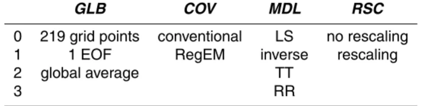
The details are found in a supplement (http://www.clim-past-discuss.net/2/357/2006/ cpd-2-357-2006-supplement.zip). Table 1 illustrates the various settings.

By varying the criteria a set of 48 model variants or flavors is defined, identifiable by a 10

quadruple from [0,2]_×[0,1]_×[0,3]_×[0,1] as in B ¨urger and Cubasch, 2005. For example,

the MBH98 method corresponds to variant 1011 and Rutherford et al., 2005 to 0130.

4 Resampling proxies and temperature

Suppose we have fixed a calibration setCconsisting ofPandTvalues, and we want to

build one of the modelsMabove. SinceMdoes not explicitly contain the time variable,

15

it only depends on the setCof selectedPandTvalues, and not on their ordering. In

an ideal world, any other samplingC′would result in the same modelM(C′)=M(C). In

the real world of statistics there are sampling errors, and the estimatesM(C) vary more

or less about the “true” model M– if such model exists at all. We assume M exists,

and for each of the above flavors we are now estimating it along with a corresponding 20

uncertainty range. We are confident that 100 random setsC are sufficient to obtain

reasonable estimates.

Let the full, 127-year longP–Trecord be given as (Pi, Ti, i∈I). A “random” calibration

set is defined by picking a random permutationπ:I→I and letting

C(π)=

i _∈I _| π(i)_≤n/2 (1) 25

(8)

CPD

2, 357–370, 2006

reconstructions

Title Page

Tables Figures

◭ ◮

Back Close

Full Screen / Esc

(nbeing the length ofI). This divides the original record into two sets, calibrationC(π)

and validation V(π)=I \C(π), of roughly equal size. Applying now the 4 steps from

above yields 48 flavors per π, and doing this 100 times generates for each flavor a

distribution of 100 regression experiments.

Their predictive power is evaluated in terms of NHT, calculated from observed, x,

5

and predicted values (from the validation part), ˆx, of the 219 grid points. In accordance

with (Lorenz, 1956) and (Briffa et al., 1988) we use the scores

RE =1− D

( ˆx₋x)2E

D

(x₋x¯_c)2E

; CE =1−

D

( ˆx₋x)2E

D

(x₋x¯_v)2E

, (2)

with brackets indicating expectation. They are only distinguished by the di_fferent

refer-ence value of calibration and validation mean, ¯x_c and ¯x_v, respectively.

10

Their distribution is depicted in Fig. 1. For each flavor, the scores from the random

calibrations show a considerable spread, but that spread is remarkably similar forRE

and CE. This demonstrates that, in fact, both measure the same thing, and possible

differences merely reflect sampling properties. Most flavors have difficulty predicting

the entireTgrid (0xxx), except maybe the variant 0130 favored by Mann et al. (2005).

15

Overall, prefiltering the T grid using EOF truncation noticeably improves the

perfor-mance. Here also the use of RegEM gives a few percent of additional score. Interest-ingly, using NHT itself as a predictand (2xxx) does not seem to be favorable as many calibrations show very poor performance, thus increasing the uncertainty. Most of the higher scores lie in a range somewhere between 10% and 30%. Given this uncertainty, 20

it is hard to pick one flavor as optimal. From the Figure, the flavor 1120 shows the best results with a moderate uncertainty, scoring between 15% and 40%.

The additional dots in the Figure represent the “classical” calibration C0 of the

pe-riod 1902–1980 (with validation 1854–1901) used in previous studies. C₀ obviously

assumes the role of an outlier, in a positive sense forRE and in a negative one forCE.

25

WhileRE values approach 60% (for 1120) theCE values are negative throughout. It

(9)

CPD

2, 357–370, 2006

reconstructions

Title Page

Tables Figures

◭ ◮

Back Close

Full Screen / Esc

Interactive Discussion appears that in the same sense that that particular calibration rewards trended

predic-tors with highRE values it penalizes them with smallCE scores. In other words: the

trend (which is “invisible” toCE) dominates calibration and validation.

Note that the RegEM variant 0130 only scores 30% for C0. This method, whose

millennial performance is assessed here for the first time, was advertised by Mann et 5

al. (2005) and earlier to replace the original MBH98 method 1011, which scores almost

50% in our emulation. Hence, even ifC0did not reflect a sampling bias, our results do

not suggest a transition to that variant.

The nonsense predictor mentioned above (number of available grid points) scores

RE=46% (andCE=−23%), which is more than any of the flavors ever approaches in

10

the 100 random samples. And it is not unlikely that other nonsense predictors score

even higher. On this background, the originally reported 51% of verificationRE are

hardly significant. This has already been claimed by McIntyre and McKitrick (2005b)

in a slightly different context. In addition to that study, we have derived more stable

estimates of verifiable scores for a whole series of model variants, the optimum of 15

which (1120) scoring withRE=25%_±7% (90% confidence).

Note that such a random calibration set Cvery likely destroys the original temporal

ordering of thePandTseries (albeit synchronously for both), along with the observed

20th century warming trend. To someone more used to dynamical models (which

con-tain the time variable explicitly) this “shuffling” may appear irritating as it would destroy

20

the main “physical process” that one attempts to reflect. We therefore emphasize that empirical models of this kind do in no way contain or reflect dynamical processes other than can be sampled in instantaneous covariations between variables. The trend may be an integral part of such a model, but only as long as it represents these covariations.

One might nevertheless attempt to “help the sampling” by picking only thoseCthat

25

preserve contiguous time spans of a length typical forP–T interactions, say 5 years.

We have tested for 1, 5, and 10 years, but did not observe significant changes to Fig. 1 apart from a slight decrease of skill and increase of spread (see supplement). For longer time scales the diminishing degrees of freedom is a limiting factor.

(10)

CPD

2, 357–370, 2006

reconstructions

Title Page

Tables Figures

◭ ◮

Back Close

Full Screen / Esc

5 Conclusions

Previous estimates of climate reconstruction skill, especiallyRE, are founded on the

particular partitioning into calibrating and validating portions of the trended instrumen-tal period, and thus mainly reflect sampling properties. This leaves very few degrees of freedom, and they can easily be matched by nonsense regressors. To accommodate 5

for this sampling bias we have proposed a strategy that is based on repeated resam-pling of the instrumental period, similar to other techniques not unusual in statistical estimation theory (cf. Efron and Gong, 1983).

The results pose a number of questions. (1): Are the results representative, i.e. are

100 experiments per flavor enough to estimate the uncertainty? Given the huge

10

amount of possible permutations of 127 years the number of 100 experiments is quite small. On the other hand, if there is sense at all behind the idea to distill an empirical model out of the 127 proxy and temperature records, sampling 100 is probably suf-ficient. The 1902–1980 calibration, as an outlier, is very hard to “sample” randomly. – (2): Are we in a position to advertise a “best” flavor? The flavor 1120 – EOF trun-15

cated predictand, RegEM, TT regression, and no rescaling – with anRE of 25%_±7%

shows the highest scores; but other scores (1011, 1101) are well within the uncertainty

bound. – (3): Are 25%RE enough to decide the millennial NHT controversy? This is

the crucial question. 25%RE translates to an amplitude error of √(100–RE) _∼85%.

If one were to focus the controversy into the single question: Was there a Medieval 20

Warm Period (MWP) and was it possibly warmer than recent decades? – we doubt that question can be decided based on current reconstructions alone.

Acknowledgements. This work was funded by the EU project SOAP.

References

Briffa, K. R., Jones, P. D., Pilcher, J. R., and Hughes, M. K.: Reconstructing summer tempera-25

(11)

CPD

2, 357–370, 2006

reconstructions

Title Page

Tables Figures

◭ ◮

Back Close

Full Screen / Esc

Interactive Discussion Arctic Alpine Res., 20, 385–394, 1988.

B ¨urger, G. and Cubasch, U.: Are multiproxy climate reconstructions robust?, Geophys. Res. Lett., 32, L23711, doi:10.1029/2005GL0241550, 2005.

B ¨urger, G., Fast, I., and Cubasch, U.: Climate reconstruction by regression – 32 variations on a theme, Tellus A, 58(2), 227–235, doi:10.1111/j.1600-0870.2006.00164.x, 2005.

5

Cook, E. R. and Kairiukstis, L. A.: Methods of dendrochronology: applications in the environ-mental sciences, Kluwer Acad. Publ., 394 pp., 1990.

Cook, E. R., Briffa, K. R., and Jones, P. D.: Spatial regression methods in dendroclimatology: a review and comparison of two techniques, Int. J. Climate, 14, 379–402, 1994.

Dempster, A., Laird, N., and Rubin, D.: Maximum likelihood estimationfrom incomplete data via 10

the EM algorithmm, J. Royal Stat. Soc. B, 39, 1–38, 1977.

Efron, B. and Gong, G.: A Leisurely Look at the Bootstrap, the Jackknife, and Cross-Validation, Am. Stat., 37(1), 36–48, 1983.

Fierro, R. D., Golub, G. H., Hansen, P. C., and O’Leary, D. P.: Regularization by Truncated Total Least Squares, SIAM J. Sci. Computing, 18(4), 1223–1241, 1997.

15

Hoerl, A. E.: Application of ridge analysis to regression problems, Chem. Eng. Prog., 58, 54– 59, 1962.

Huybers, P.: Comment on “Hockey sticks, principal components, and spurious significance”, Geophys. Res. Lett., 32, L20705, doi:10.1029/2005GL023395, 2005.

Jones, P. D. and Briffa, K. R.: Global surface air temperature variations during the twentieth 20

century: Part 1, spatial, temporal and seasonal details, The Holocene, 2, 165–179, 1992. Legates, D. R. and McCabe, G. J.: Evaluating the use of “goodness of fit” measures in

hydro-logic and hydroclimatic model validation, Water Resour. Res., 35, 233–241, 1999.

Lorenz, E. N.: Empirical orthogonal functions and statistical weather prediction, Sci. Rept. No. 1, Dept. of Meteorol., M. I. T., 49 pp., 1956.

25

Mann, M. E. and Rutherford, S.: Climate reconstruction using “Pseudoproxies”, Geophys. Res. Lett., 29(10), 139, 2002.

Mann, M. E., Bradley, R. S., and Hughes, M. K.: Global-scale temperature patterns and climate forcing over the past six centuries, Nature, 392, 779–787, 1998.

Mann, M. E., Bradley, R. S., and Hughes, M. K.: Northern Hemisphere temperatures during 30

the past millennium: Inferences, uncertainties, and limitations, Geophys. Res. Lett., 26(6), 759–762, 1999.

Mann, M. E., Rutherford, S., Wahl, E., and Ammann, C.: Testing the Fidelity of Methods Used

(12)

CPD

2, 357–370, 2006

reconstructions

Title Page

Tables Figures

◭ ◮

Back Close

Full Screen / Esc

Interactive Discussion in Proxy-Based Reconstructions of Past Climate, J. Climate, 18, 4097–4107, 2005.

McIntyre, S. and McKitrick, R.: Corrections to the Mann et al. (1998) Proxy Data Base and Northern Hemispheric Average Temperature Series, Energy Environ., 14(6), 751–771, 2003. McIntyre, S. and McKitrick, R.: Hockey Sticks, Principal Components and Spurious

Signifi-cance, Geophys. Res. Lett., 32(3), L03710, 2005. 5

McIntyre, S. and McKitrick, R.: The M&M Critique of the MBH98 Northern Hemisphere Climate Index: Update and Implications, Energy Environ., 16(1), 69–100, 2005.

Murphy, A. H. and Winkler, R. L.: A general framework for forecast verification, Mon. Wea. Rev., 115, 1330–1338, 1987.

Nash, J. E. and Sutcliffe, J. V.: River flow forecasting through conceptual models – Part I – A 10

discussion of principles, J. Hydrol., (10), 3, 282–290, 1970.

Rutherford, S. and Mann, M. E.: Climate Field Reconstruction under Stationary and Nonsta-tionary Forcing, J. Climate, 16, 462–479, 2003.

Rutherford, S., Mann, M. E., Osborn, T. J., Bradley, R. S., Bri_ffa, K. R., Hughes, M. K., Jones, P. D.: Northern Hemisphere Surface Temperature Reconstructions: Sensitivity to Methodology, 15

Predictor Network, Target Season and Target Domain, J. Climate, 18, 2308–2329, 2005. Schneider, T.: Analysis of incomplete climate data: Estimation of mean values and covariance

matrices and imputation of missing values, J. Climate, 14, 853–871, 2001.

von Storch, H., Zorita, E., Jones, J. M., Dmitriev, Y., and Tett, S. F. B.: Reconstructing Past Climate from Noisy Data, Science, 306, 679–682, 2004.

20

Wahl, E. R. and Ammann, C. M.: Robustness of the Mann, Bradley, Hughes reconstruction of Northern hemisphere surface temperatures: Examination of criticisms based on the nature and processing of proxy climate evidence, Climatic Change, in press, 2006.

Wilks, D. S.: Statistical Methods in the Atmospheric Sciences. An Introduction. Academic Press, San Diego, 467 pp., 1995.

25

Wolock, D. M. and McCabe, G. J.: Explaining spatial variability in mean annual runoff in the conterminous United States, Climate Res., 11, 149–159, 1999.

(13)

CPD

2, 357–370, 2006

reconstructions

Title Page

Tables Figures

◭ ◮

Back Close

Full Screen / Esc

Table 1.The 3_×2_×4_×2=48 regression flavors.

GLB COV MDL RSC

0 219 grid points conventional LS no rescaling 1 1 EOF RegEM inverse rescaling

2 global average TT

3 RR

(14)

CPD

2, 357–370, 2006

reconstructions

Title Page

Tables Figures

◭ ◮

Back Close

Full Screen / Esc

Interactive Discussion 0000 0001 0010 0011 0020 0021 0030 0031 0100 0101 0110 0111 0120 0121 0130 0131 1000 1001 1010 1011 1020 1021 1030 1031 1100 1101 1110 1111 1120 1121 1130 1131 2000 2001 2010 2011

-100 -80 -60 -40 -20 0 20 40 60

RE [%]

-100 -80 -60 -40 -20 0 20 40 60

CE [%]

Fig. 1. The verification scores RE and CE of all 48 flavors. A bar indicates the spread of all 100 experiments using randomly resampled calibrations, a black dot the experiment with 1902–1980 calibration.