Analysis and simulation of AGVS routing strategies using V-REP

F

E

U

P

Analysis and simulation of AGVS

routing strategies using V-REP

Luís Filipe de Lemos Miranda

Mestrado Integrado em Engenharia Mecânica Supervisor: Manuel Romano dos Santos Pinto Barbosa Co-Supervisor: António Manuel Ferreira Mendes Lopes

Analysis and simulation of AGVS routing strategies using

V-REP

Luís Filipe de Lemos Miranda

Mestrado Integrado em Engenharia Mecânica

Abstract

An Automated Guided Vehicle System (AGVS) is a modern solution for material transportation in a industrial context, where vehicles, with varying degrees of autonomy, can independently move around the layout. The routing problem, a part of fleet management, concerns specifically the issue of how a vehicle can get from a point of origin to a destination and when multiple vehicles are present, it becomes quite complex to solve. Due to the highly dynamic nature of several vehicles moving simultaneously, the wrong routing strategy can lead to much higher delivery times and distances and even deadlocks. Due to its complexity, usually there is not a single solution to the problem, and thus, simulations become very important. For this purpose, V-REP, a robotic systems simulator, is used.

The first step towards a complete simulation is the creation of a layout. For this dissertation, free range vehicles, which move freely inside their confined spaces, are used. Using the provided 3D modeller, the size, objects, obstacles and nodes are defined, as well as the vehicle, a simple round shape. To control all aspects of the simulation, three scripts were created: manager script (assigns tasks to the vehicles), vehicle script (controls the vehicle movements, one for each) and the totals script (gathers all data to produce the outputs).

Since the vehicles are free range, a special focus was given to strategies where the paths are found using path finding algorithms, using the already included in V-REP, Open Motion Planning Library (OMPL), which allows quick and easy testing of many algorithms. To better understand V-REP and the OMPL, a first case with a single vehicle is created, after which a transition to a multi-vehicle situation is made.

Finally, the multi-vehicle routing strategies are implemented and tested. Most of the strategies use mainly the OMPL, while one of them uses a exhaustive node search approach. Each strategy must complete a given task list and the number of vehicles increases from one to six vehicles. From the data obtained, which concerns both the in-simulation parameters (time and distance) and also how V-REP performs while executing them, each strategy is analysed along with an overall comparison.

In general, it was possible to implement different routing strategies in a multi-vehicle type problem, taking advantage of V-REP functionalities for modelling the various elements, including layout facilities, vehicles, path planning and routing strategies. The main limitation is related to the simulation speed performance, which can be expected to degrade with the size and complexity of the system. Taking into account the extensive capabilities of V-REP, it might be more appropriate to use it to simulate more localized navigation problems regarding selected paths (incorporating the vehicle’s dynamic and kinematic models), rather than complex routing problems with a high number of vehicles.

Resumo

Um AGVS (Sistema de Veículos Guiados Autonomamente) é uma solução moderna para o trans-porte de materiais num contexto industrial, onde os veículos, com diferentes níveis de autonomia se movem independentemente no espaço. O problema de routing, uma parte da gestão de frota, relaciona-se diretamente com a questão de como deve um veículo ir desde um ponto de origem até um de destino e quando múltiplos veículos estão presentes, torna-se um problema bastante complexo. Devido à natureza altamente dinâmica de ter vários veículos em movimento simultane-amente, a estratégia de routing errada pode levar a tempos e distâncias de entrega elevados e até bloqueios do sistema. Devido à sua complexidade, não existe normalmente uma solução única para este problema e, portanto, as simulações tornam-se bastante importantes. Para este propósito, o V-REP, um simulador de sistemas robóticos, foi usado.

O primeiro passo para uma simulação completa é a criação do espaço de trabalho. Para esta dissertação, foi escolhido um espaço onde os veículos se movem livremente dentro das suas áreas delimitadas. Usando o modelador 3D fornecido, o tamanho, objetos, obstáculos e nodos são definidos, tal como o veículo, uma simples forma redonda. Para controlar todos os aspetos da simulação, são criados três scripts: manager script (onde as tarefas são atribuídas), vehicle script (controla os movimentos de veículo, um para cada) e o totals scripts (que reúne toda a informação para produzir os outputs).

Sendo o espaço de movimento livre, foi dado um foco especial a estratégias onde os caminhos são encontrados usando algoritmos de pesquisa de caminhos, usando a Open Motion Planning Library (OMPL), já incluída no V-REP, que permite testar e alterar facilmente vários algoritmos. Para entender melhor o V-REP e a OMPL, é criado um primeiro caso com apenas um veículo, após o qual é feita uma transição para uma situação de múltiplos veículos.

Finalmente, as estratégias de routing de múltiplos veículos são implementadas e testadas. A maioria das estratégias usa principalmente a OMPL, enquanto uma delas usa uma técnica de pesquisa exaustiva de nodos. Cada estratégia tem de completar uma lista de tarefas, com o número de veículos a variar de um a seis. Os dados obtidos referem não só os parâmetros de simulação (tempo e distância), mas também o próprio desempenho do V-REP ao executar as estratégias. É feita uma análise para cada estratégia, tal como uma comparação entre todas.

De modo geral, foi possível implementar diferentes estratégias de routing com múltiplos veícu-los, aproveitando as funcionalidades do V-REP para modelar diferentes elementos, tais como o espaço de trabalho, veículos, planeamento de rotas e estratégias de routing. A principal limitação encontrada está relacionada com a velocidade de execução das estratégias, que, tal como esper-ado, piora com o aumento do tamanho e complexidade do sistema. Tendo em conta as muitas capacidades do V-REP, talvez seja mais apropriado para a simulação de problemas de navegação local (incorporando os modelos dinâmicos e cinemáticos dos veículos), do que para problemas complexos de routing com elevado número de veículos.

Agradecimentos

Aos meus orientadores, Professor Manuel Romano Barbosa e Professor António Mendes Lopes, pela ajuda e orientação dada ao longo deste trabalho.

A todos os colegas e professores desta faculdade que me acompanharam ao longo de todo o curso.

Aos meus amigos, que sempre me incentivaram e me ajudaram a completar esta dissertação. Aos meus pais, por sempre me apoiarem e me permitirem chegar a este ponto na minha vida e a quem dedico esta dissertação.

À minha namorada, por sempre me aturar e encorajar, sem nunca me deixar desistir, numa altura tão difícil, como foi este trabalho.

Luís Filipe Miranda

“Whenever you feel like criticizing any one," he told me, "just remember that all the people in this world haven’t had the advantages that you’ve had.”

F. Scott Fitzgerald, The Great Gatsby

Contents

1 Introduction 1

1.1 The Routing Problem . . . 1

1.2 Goals . . . 2

1.3 Dissertation Structure . . . 2

2 AGV Systems 5 2.1 Automated Guided Vehicle System . . . 5

2.1.1 Vehicles . . . 6

2.1.2 Layouts . . . 7

2.1.3 AGVS Control Architecture . . . 9

2.1.4 AGV Management . . . 10

2.2 Routing Problem and Path Planning Algorithms . . . 11

2.3 Simulators . . . 17

2.3.1 Webots . . . 17

2.3.2 Gazebo . . . 18

2.3.3 V-REP . . . 18

2.3.4 Simulators Comparison . . . 19

3 Single Vehicle Routing Problem in V-REP 21 3.1 V-REP . . . 21

3.1.1 Scene Objects . . . 22

3.1.2 Calculation Modules . . . 25

3.1.3 Control Mechanisms . . . 28

3.1.4 Simulation . . . 30

3.2 Single Vehicle System Model . . . 31

3.2.1 Layout . . . 31

3.2.2 Vehicles . . . 33

3.2.3 Manager Script . . . 34

3.2.4 Vehicle Script . . . 34

3.2.5 Totals Script and Other Output Files . . . 38

3.3 Single Vehicle System Tests . . . 38

3.3.1 Simulation Time Step . . . 40

3.3.2 OMPL Parameters . . . 40

3.3.3 Straight Line Tests . . . 41

3.3.4 Obstacle Avoidance Tests . . . 42

3.3.5 Pose Tests . . . 44

3.4 Conclusions . . . 46 ix

4 Modelling a Multi-vehicle Problem in V-REP 49

4.1 From Single Vehicle to Multi-Vehicle . . . 49

4.1.1 Layout . . . 49

4.1.2 Algorithms Performance in a Single Vehicle Case . . . 51

4.2 Multi-Vehicle Routing Strategies . . . 57

4.2.1 First Strategy . . . 58 4.2.2 Second Strategy . . . 61 4.2.3 Third Strategy . . . 63 4.2.4 Fourth Strategy . . . 67 4.2.5 Fifth Strategy . . . 69 4.2.6 Strategies Comparison . . . 71 4.3 Conclusions . . . 74

5 Conclusions and Future Work 75 5.1 Conclusions . . . 75

5.2 Future work . . . 76

List of Figures

2.1 Unit load AGV for transporting containers from Konecranes Gottwald [5] . . . . 6

2.2 Omnidirectional AGV used to move shelves in a warehouse, lifting them from below, from Amazon Robotics [8] . . . 7

2.3 A few common layouts, where M represents a machine or load/unload station . . 8

2.4 Example of a common AGV control architecture . . . 9

2.5 Example of a system monitor software, Q-View by Savant [13] . . . 10

2.6 Comparison between visibility graph and Voronoi diagram of the same space [21] 13 2.7 Flowchart describing how Dijkstra’s algorithm explores a graph . . . 15

2.8 Example of a path finding task using a PRM algorithm, in [27] . . . 16

2.9 Example of a path finding task using a RRT algorithm, in [27] . . . 16

2.10 Webots graphical environment [33] . . . 18

2.11 Gazebo graphical environment [34] . . . 19

2.12 Example of a V-REP scene . . . 20

3.1 Hierarchy of the NAO robot implementation in V-REP, composed of shapes, dum-mies, joints, force sensors and vision sensors . . . 24

3.2 Demonstration of how bezier interpolation works in V-REP [37] . . . 25

3.3 User window for the calculation modules, with the dynamics module selected . . 26

3.4 Example of an OMPL task in an embedded script . . . 28

3.5 V-REP control architecture demonstrating how each control mechanism integrates with the others [37] . . . 29

3.6 The created components that make up the system (scene) . . . 32

3.7 Relationship between the scripts, vehicles and output files. The communication between scripts is done using signals . . . 32

3.8 Location of the stations in the layout . . . 33

3.9 Flowchart describing the manager script for n vehicles . . . 35

3.10 Flowchart demonstrating the vehicle script . . . 37

3.11 Path performed by the vehicle in the first test case . . . 39

3.12 Graphical visualisation of the results for all algorithms in pose mode, using the two longest times . . . 45

4.1 Multi-vehicle layout, made up of 21 nodes, including load/unload stations and intersections . . . 50

4.2 Representation of the multi-vehicle layout, with closed walls and cells, forming 2 m corridors . . . 52

4.3 All calculated paths using RRT* in the path length comparison test . . . 55

4.4 Two of the obstacle placement configurations used in the obstacle avoidance test . 56 4.5 Overview of the strategies tested . . . 58

4.6 Flowchart describing the second strategy vehicle behaviour . . . 62 4.7 Scatter plot showing the time and distance for all successful cases, labels are in

List of Tables

3.1 Vehicle average speed over five runs for different simulation time steps . . . 40

3.2 Impact of search and simplification time on the total calculation time for the com-plete path . . . 41

3.3 Distance and calculation time over five runs for different algorithms and varying search times in a straight line (station 8 to 5) . . . 42

3.4 Distance and calculation time over five runs for different algorithms and varying search times in an obstacle avoidance path (station 5 to 2) . . . 43

3.5 Distance and calculation time over five runs for different algorithms and varying search times in a straight line (station 8 to 5) in pose mode . . . 45

3.6 Distance and calculation time over five runs for different algorithms and varying search times in an obstacle avoidance path (station 5 to 2) in pose mode . . . 46

4.1 Number of necessary attempts to find a successful path between node 21 and node 1 with 1.5 m and 2 m wide corridors . . . 53

4.2 Comparison between the length of calculated paths and minimum straight line dis-tance, connecting the twelve load/unload stations, using RRT* with a 10 s search time . . . 54

4.3 Comparison between the length of calculated paths and minimum straight line distance, connecting the twelve load/unload stations, using Lazy PRM* with a 10 s search time . . . 54

4.4 Length of path found depending on the number of present obstacles, for both RRT* and Lazy PRM* . . . 57

4.5 Results for the first strategy: one to six vehicles . . . 60

4.6 Results for the second strategy: one to six vehicles . . . 64

4.7 Results for the third strategy: one to six vehicles . . . 66

4.8 Results for the fourth strategy: one to six vehicles . . . 68

4.9 Results for the fifth strategy: one to six vehicles . . . 70

Abbreviations and Symbols

AGV Automated Guided Vehicle

AGVS Automated Guided Vehicle System RRT Rapidly-exploring Random Tree RRT* Rapidly-exploring Random Tree star PRM Probabilistic RoadMap

PRM* Probabilistic RoadMap star Lazy PRM* Lazy Probabilistic RoadMap star OMPL Open Motion Planning Library ROS Robot Operating System CAD Computer-Aided Design

V-REP Virtual Robot Experimentation Platform

Chapter 1

Introduction

1.1 The Routing Problem

The routing problem is found in the context of vehicle and traffic management and it specifically concerns the issue of how to go from a point of origin to a destination. This problem can be found in a multiple vehicle situation, where the complexity increases as it has to guarantee a successful path, one that connects the origin and destination, for each of the vehicles in a efficient and timely manner. While it may be applied to a multitude of situations, such as urban traffic or delivery trucks, in this case it concerns the routing of multiple automated guided vehicles in an industrial setting. An automated guided vehicle system (AGVS) is comprised not only by the vehicles but also by the fleet management, control architecture and all other elements necessary for a fully working system [1].

The vehicles, which are a type of mobile robots, can vary according to the navigation and localization methods employed and also the type of task they are designed for. These vehicles are integrated in a larger network that allows communication between the vehicles as well as to a central computer system that receives and provides the necessary information for the vehicles to complete the orders. The management system also plays a major part in the larger AGVS and is responsible for, among other things, the dispatching, allocation and scheduling of vehicles, as well as the routing and path selection. When there is a high number of vehicles involved, the management problems become more dynamic and complex, and thus, a proper strategy can have a considerable impact on the system’s performance.

A solution to the routing problem is dependent on many factors, e.g. the number of vehi-cles, the autonomy and movement capabilities of the vehivehi-cles, the layout, including the load and unloading areas, occupied space and free workspace available for the vehicles to move, among others. All of these variables can combine in innumerable ways, making the solution to the rout-ing problem not a srout-ingle one, but instead one that depends on the specific case. The difficulties of a multi-vehicle scenario arise from the highly dynamic behaviour caused by the ever changing position of the vehicles and other obstacles. Due to this, the solutions usually rely on a previously

chosen set of rules that provide a route for each vehicle from start to finish and possible solutions to any problems that can arise during movement, such as blocked areas or traffic congestions [2].

Due to the complexity and high cost of implementing or changing an AGVS in a factory or other industrial setting, system simulations are an important and valuable step, both before its creation and during its use. This can help in determining the most efficient layout scheme, the management and routing strategies that should be used, the number of vehicles required and other parameters [3]. The software used in this work is V-REP due to its public availability for students and its capabilities for creating graphic environments, calculation modules and programming abil-ities, that allow for the implementation, testing and visualisation of different routing strategies.

1.2 Goals

The main objective for this work is to create a model of an automated guided vehicle system, capable of working under different routing strategies and to determine how adequate is V-REP for this goal. For this purpose, the V-REP software must be explored and analysed as to determine how to create an environment that allows for the analysis of the various routing strategies. The goals for these models are:

• Creation of various layouts, including the occupied and the free space for the vehicle to move, as well as the location of the stations;

• Selection of the number of vehicles to be used in the simulation; • Specification of the transport tasks to be completed;

• Implementation of different routing strategies;

• Extraction of data from the simulations, to further analyse the advantages and disadvantages of the different strategies.

With the creation and combination of these features in V-REP scenes, a multitude of possibil-ities can be created to compare routing strategies under different conditions.

1.3 Dissertation Structure

This dissertation is structured in five chapters. Subsequent to this introduction comes Chapter2: AGV Systems, where it is presented what an automated guided vehicle system is and how it works, from the vehicles themselves to fleet management and the control structure. What the routing problem is and its possible solutions, are addressed in more detail. In conclusion, it is given an overview of some commercially available simulators, including V-REP, and a comparison between them.

The third chapter, Chapter3: Single Vehicle Routing Problem in V-REP, concerns, in the first section, the functionalities and possibilities of V-REP, with a special focus on the elements that can

1.3 Dissertation Structure 3

assist the creation of the system and are used throughout this work, such as paths and embedded scripts. A model of a single vehicle system is created, along with a delineation of the composing elements, particularly the scripts. This system is then tested to validate the elements created and to define a structure for modelling a multiple vehicle routing problem.

Chapter 4: Modelling a Multi-vehicle Problem in V-REP, explores the possibilities of introduc-ing more vehicles to the system and how this impacts the routintroduc-ing problem. The different layouts used for the tests are described, as well as the new routing strategies implemented. Additional scripts and elements added to the scene are also specified, along with the data produced from the test cases. The information obtained is then analysed and the results from different strategies are compared for a conclusive evaluation.

Finally, in Chapter 5: Conclusions, the results and conclusions from the work are summarized and presented in a global context, focusing on the capabilities of using V-REP for the specific pur-pose of simulating an automated guided vehicle system and applying different routing strategies to it. Possible future work and expansions to the system are also discussed.

Chapter 2

AGV Systems

This chapter addresses what an automated guided vehicle system is and how it works. The vehi-cles, possible layouts, path planning algorithms and the system in which they are integrated in are presented. Then, the routing problem is presented along with some common solutions. Lastly, a brief comparison between simulators is made.

2.1 Automated Guided Vehicle System

Robotics is currently one of the most appealing areas in the industrial world and a big part of it are mobile robots. Of these, automatic guided vehicles take a special interest by being a flexible and modern solution for material flow, offering new possibilites in many industrial applications, which has been used for more than fifty years. While usually an AGV is seen as a lesser mobile robot, in terms of abilities and independence, nowadays AGVs are becoming smarter and more autonomous, as they benefit from the technical developments of modern robots. Due to the ad-vancements in the vehicles technology, more manufacturers worldwide are opting to implement AGVS in their factories. By 2008, over 27,500 vehicles in 3,300 AGV systems were installed in Europe and the global number is expected to continue rising, in part due to a growth in interest from China [4]. While this number may be small when compared to other robotic systems com-ponents, manipulators or industrial robots for example, it is partly explained by the relatively high cost and difficulty to implement.

The most common use of an AGV is in a factory environment and the most usual task is material handling and transportation from one place to another. Moving products is a task that adds no value to them and where a lot of resources are spent. Because of this, it is very important for the transportation to be done in the most efficient and economical way possible, and thus, it is necessary to use the best strategy in navigation and routing.

An AGVS is composed not only by its tangible parts, such as the vehicles and the layout, but also by its intangible elements, for instance, the control architecture and fleet management. The vehicles and the layout are what defines which tasks can be performed by the system, while control

architecture and fleet management are in charge of assigning the orders to the vehicle and making sure the paths are successfully completed.

2.1.1 Vehicles

The vehicles used in AGV systems can be of many types and the choice depends on the kind of transportation task to be completed. Some commonly available vehicles are:

• Forklifts; • Tow vehicles;

• Unit load vehicles (figure2.1);

• Special application vehicles (figure2.2).

Figure 2.1: Unit load AGV for transporting containers from Konecranes Gottwald [5]

The methods used to allow an AGV to navigate autonomously have changed throughout the years, as the sensor technology used in the vehicles and environments has improved. In earlier versions, a more rigid approach was used, such as using a conducting wire embedded in the floor or reflective paint, which the vehicles would follow [6]. These methods had the problem of requiring alterations to the environment and were more intrusive and difficult to modify.

A modern alternative is to use wireless navigation. Initially this was done by using markers, such as a laser scan on top of the vehicle and reflective markers. By triangulating the positions of the markers and comparing it with the positions stored in the memory it can localise where the vehicle is [7]. The current version of this wireless technology is inertial navigation, which uses a gyroscope and an accelerometer for each axis of a three coordinate system. By starting from

2.1 Automated Guided Vehicle System 7

a known position and measuring the internal movements, it can get an accurate reading of the current position. It can also be aided by floor markers, such as QR codes [8] or magnets, to assure a correction of the positioning errors within a much more precise range.

The kinematic design found in these vehicles are usually of three basic types [9]:

• Differential control: two drive wheels vary their speed independently, in order to turn and move the vehicle, supported by swivel caster wheels;

• Steered wheel control: turns one or more guiding wheels along with other traction or support wheels, similar to normal cars;

• Omnidirectional vehicles: uses wheels that allow movement in all directions and function in a way similar to differential control. This allows the vehicle to rotate around its center and move sideways. An example can be seen in figure in figure2.2.

Figure 2.2: Omnidirectional AGV used to move shelves in a warehouse, lifting them from below, from Amazon Robotics [8]

2.1.2 Layouts

The layout of a factory is how the workspace is defined, not only by its size, but also by the location of pickup/drop-off points, static obstacles, area limitations and, in case they exist, the pre-defined paths.

The first step in a layout is defining the location of the load/unload stations. Some common arrangements are [10]:

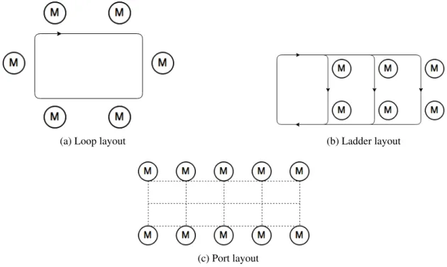
• Straight line; • Loop (figure2.3a); • Ladder type (figure2.3b);

• Custom design (figure2.3c).

A possible custom design is similar to the one found in ports, where the stations are located in two rows opposite from each other for loading and unloading. Another layout is a grid, where the stations are located in the middle of the branches.

(a) Loop layout (b) Ladder layout

(c) Port layout

Figure 2.3: A few common layouts, where M represents a machine or load/unload station

After placing the stations, a decision regarding how the vehicles move must be made. Two possible approaches are using physically pre-defined paths (using tape-guided or wire-guided nav-igation) or free range (requires the use of smarter vehicles). If the movement is done in free range, this means that the vehicles can take any possible path connecting the two stations, using different routing rules.

When the paths are pre-defined, then the routes must be carefully chosen. The layout is usually the biggest influence on what paths can be created. For more complex layouts, the paths between stations must be designed taking into account travel distance, intersections created and possible traffic occurrences, for example. The lanes can also have one or two directions.

A viable approach is what is called a tandem configuration, where a layout consists of two or more loops. Each of these loops contain specific stations where the material can be transferred from one loop to the other and usually a single vehicle per loop. This brings the simplicity and advantages of loop layouts, such as reducing or eliminating traffic control (depending if there is more than one vehicle), to more complex layouts [11].

A feature present in some layouts are buffer areas [12]. These areas exist to help traffic and avoid deadlocks. The vehicles can move into these spaces while stopped at a station or next to an intersection so the section does not get blocked.

2.1 Automated Guided Vehicle System 9

2.1.3 AGVS Control Architecture

An automatic guided vehicle must be able to work autonomously but also along with other vehi-cles, persons and computer controlled equipment in a cooperative environment. For that, it must be fully integrated into a factory system and so it has to communicate with a manager or dispatcher system.

A common way of doing this is by having a central computer manage all the vehicles and where some decisions are made and sent to each individual one. This computer is usually con-nected to a larger company wide system, such as an WMS (Warehouse Management System) or an ERP (Enterprise Resource Planning System), and so it will receive information on a higher level, such as which products are necessary or where they can be found, but also lower level equip-ments such as PLCs (Programmable Logic Controller) (figure2.4) . This central controller will also gather all information regarding the AGV’s status such as location and availability. In some cases the central computer that receives the higher level information may be connected to other computers that each then control a part of the machines or vehicles in an hierarchical form.

Figure 2.4: Example of a common AGV control architecture

With all this information, the system can then make all the necessary decisions, regarding vehicle allocation, path planning and others. Often, the system is also able to control other parts of the environment such as doors or traffic lights. The communication between the computer and the vehicle is usually done wirelessly using Radio Frequencies or an 802.11n Wireless network (Wi-Fi) [9].

The information can be visualised in a system monitor, which can gather information about the system operation and make it easily available for the user in real time or record it for external use. The computer can display the current location of the vehicles, their path, destinations or status conditions. It can also generate performance reports regarding each AGV, station, path or whatever information is desired. Any error that occurs is also logged in the system so that it can be more easily identified and solved. With the recordings of previous operations, a more careful analysis can be done at a later date.

Companies like Savant [13] or Egemin [14] offer software capable of performing these tasks (figure2.5), which can be customised, as no two factories have the same needs and specifications. Some softwares also provide functionalities to help create the working layout by using a CAD file of the factory and placing stations and pathways [15].

Figure 2.5: Example of a system monitor software, Q-View by Savant [13]

2.1.4 AGV Management

When managing a fleet of AGVs there are considerations that need to be done regarding when and how they complete the given tasks. The three main functions are [16]:

• Dispatching: dispatching is the allocation of a specific vehicle to perform a particular task; • Routing: routing is the selection of the path each vehicle should take from a starting position

to a destination;

• Scheduling: scheduling is the determination of arrival and departure times for all vehicles, taking into account the need to avoid blocking and satisfy overall production objectives. All these aspects of an AGV system must be taken into consideration when building the simu-lation. In fact, they are interconnected problems and must all be dealt with cooperatively to ensure a smooth operation with maximum efficiency.

2.2 Routing Problem and Path Planning Algorithms 11

Dispatching

The assignment of a vehicle to a task is the first step in vehicle management, and thus, must be done carefully and in consideration of the chosen performance measures. At the start of the operation or after finishing a task, that is, when the vehicle is free of any responsibility, a task must be assigned to it.

There are two ways of looking at this problem [17]:

• The vehicle initiates the assignment: this happens when there is more than one station await-ing a vehicle. In this case, the vehicle chooses a station followawait-ing a specific heuristic, such as shortest travel distance, maximum queue size. A common rule is what is called the First Come-First Serve rule, where the vehicles are assigned to the stations in chronological order of when the call was placed;

• The station initiates the assignment: this occurs when there is more than one available idle vehicle. The vehicle is again chosen by a set heuristic, such as nearest vehicle or least utilised.

The measures used to evaluate performance are not always the same and it can be, for example, distance travelled by the vehicles or machine utilisation. In general, not a single dispatching rule is going to please all performance evaluators. One possibility is to consider multi-attribute models, for example, combining both distance of vehicle to station as well as the station output queue [18].

2.2 Routing Problem and Path Planning Algorithms

The routing problem is a very important one when managing an AGV fleet. If poorly conceived, the vehicles take a much longer path than necessary, or never even arrive, which makes the system not efficient at all. The routing issue is deeply connected to the layout of the work space, as it directly affects the number of possible paths and greatly influences the decision regarding which routing strategy to adopt.

A possible approach is to send all vehicles in a loop. This eliminates the existence of intersec-tions and, consequently, the possible collisions and blocked zones. In the case of only one vehicle per loop there is very little path planning, as there is only one possibility, entering the loop, which can move in one or both directions. If multiple vehicles are used in a loop, then, traffic problems may arise, even though at a lower complexity level than other configurations. While there is less planning, for both paths and traffic control, the distances travelled by the vehicle will, in most cases, be longer than necessary, which makes this strategy less interesting. Also, it is only pos-sible if the layout supports it. If the stations are not laid out in a way that makes a loop feapos-sible, such as having a station in the middle of others, this strategy becomes even less efficient.

A different method to routing is one where the stations are connected with pre-defined paths. By connecting the links in the mesh and moving from link to link, a path from one station to the other can be found. The rules for connecting the paths can vary, but the goal is to usually find the

shortest distance. In this scenario, the possibility of collisions, blocking and other traffic problems is much higher, such as two vehicles trying to enter the same branch or what link to choose in alternative. For these cases, a set of heuristics regarding traffic control and zone blocking must be applied. Almost any layout can support this strategy as it only requires paths connecting the stations.

The routing can also be done in a layout with no previously and phisically defined paths and in a work space that is free or with obstacles, besides other vehicles. In this case the route taken will usually be a path connecting the two stations and since the only thing to avoid is other vehicles, recalculation will only be necessary if there is another vehicle in the way. There can also be no recalculation of the paths but instead an adjustment of the times in which the vehicles leave the stations, so there are no collisions or even avoidances [19].

When conflicts arise, such as deadlocks, rules must be in place to detect and deal with them or even to avoid them altogether [2]. Intersections can be a problematic area and methods for how to deal with situations when more than one vehicle wants to cross can be implemented, such as a buffer area or something similar to a traffic light. A possible approach is called forward sensing and it uses sensors that detect the distance between the vehicle and its surroundings and stop or redirect the vehicle when the distance reaches a defined threshold [20]. This method allows the vehicles to be closer to each other and a greater density in an area, but has the drawback of usually only looking in front of the vehicle and so it is only more useful in straight paths.

Zone blocking is a technique that can help avoid deadlocks. The path is first segmented into different zones and the rule is that only one vehicle at a time can be inside the zone. A vehicle that happens to be following another must wait in the previous zone until the other vehicle has left its desired area before it can move. In static zone planning, when a vehicle reaches a zone it plans to enter, it first checks if there is already another vehicle there and if there is, then it must wait for it to leave or find a new path. If the zone planning is dynamic, then the zone can change according to flow of the traffic or where the vehicle is. The control can be done by a central station that tracks each vehicle and communicates when can they enter a zone or it can be done by the vehicles themselves. The more zones there are in the work space then the more mobility there is [2].

Path Planning Algorithms

For the vehicle to navigate in an open space configuration it must be able to find a path connecting the origin and the destination and this is where path finding algorithms prove useful. While this subject relates to any sort of map and path finding task, it can also be applied to the specific problem of AGV routing.

The first step of any path planning process is the map, a representation of the environment, which can be pre-existing or built in real time. For the algorithms to be applied, the map, possibly continuous, must first be discretised. The way in which these maps are used is what differs between strategies.

2.2 Routing Problem and Path Planning Algorithms 13

Using graph search techniques, a connectivity graph in free space is built and then searched for the best solution. The graph construction starts with a representation of both occupied and free space, which is then decomposed into a map where it is possible to apply the algorithms to [21].

Thevisibility graph (figure2.6a) is a method in which the obstacle’s vertices are connected to all other vertices that are visible, including the start and destination vertex as well. These lines are always the shortest distance possible between vertices and the algorithm’s task will be to connect the start and goal positions, using these roads, in the shortest distance possible. The Voronoi diagram (figure2.6b) takes an opposite approach and roads are placed as far as possible from the obstructions. While it is more easily executable it is also less optimal as to path length.

Exact cell decomposition is an approach where the cells, or nodes, are divided by geometric features, making it that each cell is either completely free or occupied. What matters then is the ability of the vehicle to move from one cell to the other, not where it is on the cell. Due to its complexity to implement, it is not often used in mobile robotics. On the other hand,approximate cell decomposition is one of the most popular techniques, due to its grid based representation and ease to implement. In this case, the decomposition is done by recursively decreasing the cell size, generating four new rectangles for each free cell and considering free only the ones that are fully unoccupied. This method is also known as quadtree.

(a) Visibility graph (b) Voronoi diagram

Figure 2.6: Comparison between visibility graph and Voronoi diagram of the same space [21]

The next step after building the graph is to explore it and connect the start and the goal in the best way, usually the shortest path, but other criteria can be used, such as time, energy or risk. The performance of these algorithms is also affected by the graph construction and search technique used. Since these algorithms always guarantee an optimal solution, due to exhaustively searching all possibilities, the difference between performances is how long it takes to complete the search and in what context can it be used. They can either be deterministic or randomised.

Breadth-first search begins with the start node and then explores all of the subsequent nodes by visiting all its neighbours until it reaches the destination node. The best path will be the one with the least amount of edges leading to the goal, assuming all edges are of equal length. Similar

to this algorithm is thedepth-first search, which instead of exploring the neighbours, goes to the successor node first until it reaches the deepest level [22].

Dijkstra’s algorithm [23] is nearly identical to breadth-first, but with the important consider-ation that edges may take any positive value, making the optimal path not one with the least edges but one with the least total cost. The resulting optimal path to the goal is not only valid from the start but also from any other node, allowing the vehicle to reach the goal without recomputing the solution, as long as the environment stays unaltered. A flowchart describing this algorithm can be seen in figure2.7.

The A* algorithm builds off the Dijkstra algorithm with the addition of heuristics and is mainly used in grids. The heuristic function gives more information about the cost of the move-ment. Beginning at the start cell, each neighbouring cell is ordered by lowest total cost, defined by travel plus heuristic cost, the travel cost being the distance from the start cell to the next cell and the heuristic cost the distance from any cell to the goal cell. The lowest cost node is then expanded and explored until it reaches the goal node [24].

An existing variation of A* is theD* algorithm, where the algorithm reuses previous searches into the new iterations. The advantage is if there are any changes to the environment observed by the vehicle, an entirely new solution is not necessary (as it would be with A*), only cells that were altered need to be recomputed, largely decreasing the computation time required. There is also a variation where the replanning is done anytime for both A* and D* [25].

A possible approach to path planning is sampling-based, a concept that allows for quicker and more efficient answers to planning queries, as well as being able to take into account many degrees of freedom and differential constraints. It also uses less memory than other approaches. This approach, unlike graph search techniques, does not require a special map to be previously built. The algorithms only need to know what space is free and what space is occupied, and so, no previous map building is required. The process consists of randomly placing valid vehicle configurations along the state space and then connecting these with collision free paths. This means that a larger amount of samples lead to a better solution, and as the number of samples approaches infinity a valid solution is guaranteed to be found, as long as one exists.

Aprobabilistic roadmap (PRM) [26] is one of the earliest sampling-based motion planners and more appropriate for multi-query planning. It works by randomly and uniformly placing nodes on the free space and then connecting them, thus forming a graph. Since the free space is not actually known beforehand, when a configuration is placed on the workspace it is then checked if it is valid or not, and then retained or rejected. The manner in which the state space is sampled can also be changed to find the most appropriate strategy. When the pretended number of free samples has been found, the algorithm will then try to connect each sample to a chosen number of the nearest samples. Using interpolation, if a collision free path is found, the edge is added to the roadmap. Once the graph is completed the start and goal states are connected to the nearest sample and then searched for the best solution. An example of how this works can be seen in figure2.8

Tree-based planners are another type of sampling-based planners and it is an approach many algorithms use, with rapidly-exploring random tree (RRT) being one of the more commonly

2.2 Routing Problem and Path Planning Algorithms 15

Figure 2.8: Example of a path finding task using a PRM algorithm, in [27]

found [28]. They are more suited for single-query planning. The planning starts by placing a node at the start state and from there expanding a tree by sampling the free space around it. The way this is done is what differentiates the many algorithms, each using a different heuristic. The expansion can also be biased towards the goal state for a better and quicker solution. This expanding tree method can be visualised in figure2.9

Figure 2.9: Example of a path finding task using a RRT algorithm, in [27]

A variation on some algorithms such as the RRT and PRM is theRRT* and PRM*. The appended star means that the algorithm presents optimal solutions. Due to the random nature of the sampling based algorithms, the nodes end up not being placed in a way that create the shortest possible path, but instead in a more spread out way. This star variations try to smooth out the graph by connecting nodes in shorter distances. If the number of nodes approaches infinity then

2.3 Simulators 17

the solution is guaranteed to be the shortest one possible. Other variations are possible, such as the RRT-Connect [29], where two trees are built simultaneously, one from the start and other from the goal and advance towards each other or theLazy-PRM [30] where the collision checking is reduced to a minimum to save computation time.

Potential field planning is a completely different method of path planning, where a mathe-matical function is applied to the free space. The algorithm treats the vehicle as a point under the influence of a potential field, where the obstacles are repulsive forces and the goal is an attrac-tive force. While simple and intuiattrac-tive, due to its limitations, such as the vehicle getting into trap situations and difficulty with narrow passages, it is not as commonly used [31].

2.3 Simulators

Simulators are programs that allow the user to test and create behaviours for robots and other components, without having to physically interact with them. Depending on the software and robot, some may allow for the applications created on the simulator to be transferred to the physical robot, possible for example, through ROS (Robot Operating System) [32].

Most modern simulators include a variety of features that enable realistic and useful simula-tion such as the ability to display 3D models of robots and environments, either with included modelling tools or the capability to import external models, physics engines, calculation modules and scripting of behaviours with commonly used coding languages.

The benefits of using a simulator are immense, in the way that it reduces costs, saving time and money, allowing various alternatives to be tested with no costs or risks and no down-time. It also allows the user to optimize the number of vehicles needed, the most problematic areas or what management strategies to use.

2.3.1 Webots

The software Webots was created in 1998 by Dr. Olivier Michael and is used mainly for educa-tional purposes [33]. Included in the program is a wide collection of robots, sensors and actuators. It is one of the most commonly used simulation softwares in many fields, from research on robot locomotion and simulation of adaptive behaviour to teaching and robot programming con-tests.

The software is cross-platform and supports languages like C/C++, Java, Python and MAT-LAB. The rendering is made using the OGRE engine and uses a custom version of ODE as its physics engine. It also includes an internal 3D modeller, as well as supporting ROS.

The software is proprietary and can be downloaded for free with limited functionality. To access the full version it is necessary to purchase a professional or educational license. An example of a Webots scene can be seen in figure2.10

Figure 2.10: Webots graphical environment [33]

2.3.2 Gazebo

Gazebo is a robotic simulator released in 2002, developed by Open Source Robotics Foundation [34]. It is a multi-robot simulator with dynamics, with the ability to simulate multiple robots, objects and sensors in complex environments. It is also able to generate realistic sensor feedback and interactions between objects as well as simulate rigid-body physics.

The graphics are rendered using the OGRE engine. The dynamic simulations can be made using one of the four included physics engines: ODE, Bullet, Simbody and DART. The main programming language is C++ and plugins can be developed using its own API. The simulations can be run on remote servers using TCP/IP or on a cloud.

Gazebo is open-source, available for all platforms and has a very active community, with an on-line simulation model repository, forum, wiki and library for robot applications. The same company also developed ROS, a framework for writing robot software. An example of a mobile robot in Gazebo can be seen in figure2.11.

2.3.3 V-REP

V-REP (Virtual Robot Experimentation Platform) was created by Marc Freese and first launched in 2010, making it one of the most modern simulators available [35]. It can be used for many applications such as fast prototyping, simulation of automation systems and teaching.

The software offers several calculation modules for object interaction. For dynamic inter-actions, four different physics engines are available, Bullet, ODE, Vortex and Newton. Other calculations modules are: kinematics, collision detection, mesh-mesh distance and path/motion planning.

2.3 Simulators 19

Figure 2.11: Gazebo graphical environment [34]

V-Rep allows the user to choose among various programming techniques, such as: • Embedded script, the main feature of V-REP, coded in Lua;

• Add-on, also in Lua; • Plugin, using C/C++;

• Remote API client, in C/C++, Python, Java, Matlab and Urbi.

Included in the program is a large collection of commercially available robots and sensors, as well as the ability to import new models or create them using the integrated modelling abilities. Using ROS it can also connect to actual robots.

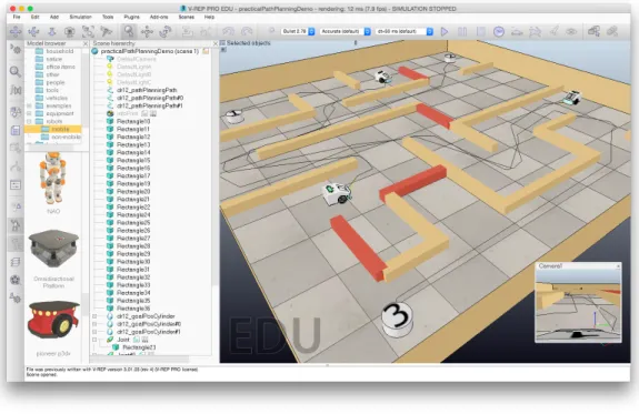
The program is cross-platform and available for free to students but must be purchased for commercial purposes. Available as well is a free player with limited capabilities. A public forum and help system are accessible on their website as well as an active on-line community. A scene containing mobile robots can be seen in figure2.12.

2.3.4 Simulators Comparison

The robotics simulators previously mentioned are some of the most commonly used and advanced available on the market. While there are other programs that can do similar tasks they have not been considered, as they are not as accessible or interesting as the others presented. While many AGVS companies offer their own simulators and managers, these are not available for public use. As to programming, Webots allows the user to choose from four different programming lan-guages, while Gazebo and V-REP mainly use only one language. Even with this limitation, V-Rep still allows for the user to employ different programming techniques.

Figure 2.12: Example of a V-REP scene

V-Rep and Gazebo have four different physics engines available and when compared to We-bots, that only has one, it shows one of the limitations of Webots.

Webots is also the only that requires a paid license, while the other two programs have full versions available for free to students.

Considering the available physics engines and calculations modules, programming techniques, versatility of both environments and robots and availability, V-REP has advantages over the other simulators. It is also more user-friendly while still including more features than the others as well as being less hardware demanding [36].

Chapter 3

Single Vehicle Routing Problem in

V-REP

In this chapter it is discussed how the V-REP software works and how it can be used to model a single vehicle system. The different components of V-REP, as well as the Open Motion Planning Library (OMPL) tool, are analysed as to how they work and can be used to the advantage of modelling any subsequent system. The single vehicle system is then built, detailing the process from the construction of the layout and vehicles to the creation of the scripts that control the model. This example is then used to test and characterize a few aspects of both V-REP and the scripts created.

3.1 V-REP

V-REP, or Virtual Robot Experimentation Platform, is a very versatile software capable of many different things within the world of robotics and due to the freedom of use given by the scripts and other programming features, almost everything you would want to do, can be done. An important aspect of V-REP is also its many calculation modules.

For clarity, the version of V-REP used in this dissertation is 3.3.2 and all simulations are executed on a computer running OS X, with 8 GB of RAM and an SSD.

V-REP is composed of three central elements that together control all aspects, graphical and logical, of a scene. The components, which are subsequently detailed, are:

• Scene objects; • Calculation modules; • Control mechanisms.

All the information in this section, and all others regarding V-REP, come from the user manual [37], the official website [35] and official forum [38].

3.1.1 Scene Objects

Scene objects are the basic building blocks of V-REP and from which other capabilities are built upon. Everything that can be visualised in a scene is an object and they can either be static or, with the help of scripts, dynamic and can be used to read data, interact with each other and many other functionalities. In a scene, objects can be in a hierarchy (e.g. figure3.1), which can influence their behaviour, or independent of other objects.

The fourteen scene objects available on V-REP are:

• Shapes: shapes are made up of triangular meshes and used for both visualisation and rigid body dynamics. Through V-REP, only primitive shapes, such as cuboids and cylinders, can be created and along with convex shapes these are optimal for a faster dynamic collision response. Shapes created using an external 3D CAD software can be imported into V-REP, first being converted into a triangular mesh. All shapes, including heightfield and random meshes, can be grouped and combined to create more complex shapes, such as vehicles and manipulators. Calculation modules, such as distance measurement and collisions, depend on shapes, and how they are modelled, to work properly. Shapes, and other objects with a physical presence on the scene, have special properties that can be customised, such as being collidable, measurable, renderable, detectable or visible. The graphical aspect of a shape can also be altered, for instance, its color or texture. The shapes can be created in the user interface, but may also be generated, and altered, during a simulation using commands like simCreatePureShape in the script;

• Joints: joints can be of four types, revolute, prismatic, spherical or screw. Joints link two or more objects together, with varying degrees of freedom, and can operate in different modes, such as force or inverse kinematics;

• Proximity sensors: proximity sensors measure the minimum distance from the sensor, which is usually attached to a different object, to any other viewable object contained within the configurable detection volume. This leads to a more realistic and continuous detection, unlike ray-type sensors;

• Vision sensors: vision sensors permit the extraction of complex data regarding an image, such as size, colors or depth. In conjunction with a plugin and integrated image processing, it is possible to filter and analyse the image;

• Force sensors: force sensors measure force and torque and are represented by rigid links.The links, depending on conditions, can break apart;

• Graphs: graphs are able to record and register a variety of data, such as time, X/Y and 3D curves;

• Lights: lights illuminate a scene, or even individual objects, and can be spotlight, directional or omnidirectional;

3.1 V-REP 23

• Cameras: cameras allow the visualisation of scene from a specific angle and position. They can also track an object or auto-fit a scene;

• Mirrors: mirrors function as real mirrors and have a clipping function;

• Dummies: dummies are used as a reference frame and commonly attached to other scene objects. Usually, scripts are attached to them as dummies have no function by themselves; • Mills: mills are customizable convex volumes that are used to simulate cutting and milling

operations;

• Paths: paths allow other objects (mainly shapes) to perform a defined movement in space (orientation and position). Can be used, for example, for conveyor belts or vehicles; • Octrees: octrees are a voxel based spatial partitioning of a shape. It can be used for faster

calculations or a simplified representation of a complex mesh;

• Point clouds: point clouds are point containers and similar to octrees. Also used for faster calculations.

Paths

Paths are a very important, and often used, scene object in all test cases created along this disser-tation and so, deserve a longer explanation.

The path object is a continuous line shaped by its control points and the successive linking of them. Each control point has certain properties, besides the more basic position and orientation, that can be altered to influence the shape of the path. One of the more important properties are the Bezier points, which dictate how the path shape behaves when connecting non straight control points, that is, the interpolation between points, in both translation and rotation, as shown in figure 3.2. Besides path shaping properties, the control point also contains information regarding virtual distance (can be useful to create a pause point along the path), relative velocity and auxiliary flags and channels.

The path can be edited manually (point by point), imported (also exported) from an external file or generated from the edge of a shape. The manual edition can be done before the simulation, using the path edition mode, or during the simulation in a script using simCreatePath and then simInsertPathCtrlPoints to insert each individual control point that form the desired path.

The only scene object that can actually perform any movement along a path is a dummy, and so, for a shape, or other object, to move along it, it must be attached to the dummy. The commands used to follow a path, such as simFollowPath or simMoveToObject, also allow the user to define a velocity and acceleration, which are associated to the command and not the path itself. The commands allow the user to choose how much of the path is completed, in a percentage, and it is not required to fully complete the path. It should also be noted that these path following commands are blocking operations, which means that while they are running, the child script is stopped and

Figure 3.1: Hierarchy of the NAO robot implementation in V-REP, composed of shapes, dummies, joints, force sensors and vision sensors

can’t complete any other operations such as collision checking or register information. A possible way to get around this limitation is to make the dummy move along the path in small increments and between motions perform any other function desired.

In V-REP, scene objects can also be models, either the object by itself or the objects below it in its hierarchy tree. If an object is flagged as being a model base, which can be done in the object dialogue box or in the script using simSetModelProperty, then it can be saved as an external file with the extension .ttm, using either the user interface or the simSaveModel command. The models may then be loaded and used in a different scene. Applying this to paths means that they may be calculated in a scene and saved for future use. Each path model is quite small in size and takes up about 50 to 70 kB.

The length of the path can be calculated in seven distinct ways, which are different combina-tions of the sum of the linear and angular variacombina-tions between control points. The method in which the distance is calculated can influence the performance of the path following commands.

3.1 V-REP 25

Figure 3.2: Demonstration of how bezier interpolation works in V-REP [37]

3.1.2 Calculation Modules

A scene object by itself does not have much use and therefore needs an algorithm or command to make it interact or move. The calculation modules are no more than algorithms that come pre-built in V-REP and can be modified and implemented through a user interface window, as seen in figure3.3. The advantage of having these modules already built-in is that these basic functions, which are often used in any simulation, require no external libraries, plugins or even coding and so makes any scene portable and easy to share. The calculations modules are also accessible by the scripts, and while they may be used exclusively through the user window, for a more complete and dynamic usage the commands available through the scripts are necessary.

The five available calculation modules are:

• Collision detection module: the collision detection module works by checking for inter-ference between shapes or collection of shapes, that is, a collision exists when there is an overlap of shapes, octrees or point clouds. This collision module is independent of collision responses from the dynamic engines;

• Kinematics module: the kinematics module works for both inverse and forward kinemat-ics of any mechanism, such as redundant, branched or closed. It supports conditional, damped/undamped and weighted resolutions, as well as collision avoidance. Also avail-able is a geometric constraint solver, that performs the same tasks as the kinematics module in a more intuitive way for the user, but is slower and less precise;

• Distance calculation module: the distance calculation module can quickly measure the minimum distance between any two meshes or collection of shapes;

• Path/Motion planning module: the path and motion planning module can handle holo-nomic and non-holoholo-nomic tasks and uses an RRT approach. While it is still available, V-REP developers no longer recommend it as it has been replaced by the OMPL plugin, which is further detailed below;

• Dynamics module: the dynamics and physics module is what allows the realistic handling of rigid body interactions, such as collisions and grasping. Four different physics engines can be used for this purpose, the Bullet Physics, the Open Dynamics Engine, the Vortex Dynamics and the Newton Dynamics. Since physics engines work mainly by using approx-imations, it is good to use more than one engine to confirm results.

Figure 3.3: User window for the calculation modules, with the dynamics module selected

Open Motion Planning Library

The Open Motion Planning Library (OMPL) is a library that includes a variety of sampling based motion planning algorithms [39]. The library itself consists of only the algorithms with no colli-sion checking or user interface, so it can be more easily implemented with other programs, such as V-REP. While it is not a calculation module, it replaces the previously existing path and motion calculation module.

The implementation of OMPL in V-REP is done with a plugin wrapping the library and is available natively in the most recent versions of V-REP. The library can only be used inside the scripts using functions during simulations and no user interface window for the library is available. To complete a path or motion planning task using this functionality, a few steps have to be taken into account.

The first step is to set a state space. The state space is the space where the algorithm will search for possible configurations. The lower and upper bounds of the search area (or volume) are set, as well as the type of state space, which can be in two or three dimensions, position or pose (position and orientation). In V-REP there are twenty five available sampling algorithms from the OMPL and although any of them can be chosen for any situation, some are more appropriate for

3.1 V-REP 27

certain tasks than others. No parameters associated with the algorithms, such as goal bias or how neighbours are connected, can be altered through V-REP, therefore, the algorithms must be used as provided.

The next step is to specify which pair of entities are not allowed to collide, such as the vehicle against itself or the vehicle against the environment for example. The start state and goal state also have to be defined. Depending on the type of state space chosen this can be only the position coordinates or the orientation as well. All these parameters are associated to a path planning task, meaning that they can be changed individually at any time, or even have different tasks in the same script. For example, the origin or destination position may be altered and then a new path calculated without having to redo all the steps, since each parameter only has to be defined once.

When all of this is specified the last step is reached, which is the computation of the task itself. The computation is made up of three parts: the solving, simplifying and interpolation of the path. The maximum time allowed for each of the searching and the simplification procedures can be specified, in seconds, as well as the number of states to be returned, that is, how many individual coordinates that make up the path. The result is a vector containing the coordinates of each state in the path in a sequential manner. Using this vector, each point can be inserted as a control point in a path object and thus making the result a continuous path that can be followed by a vehicle. An example of how these steps are implemented in code in an embedded script, using regular API functions, can be seen in figure3.4.

In case a solution is not found, the returned vector is smaller than the set number of states. To make sure a solution is found, a possible fix is to repeat the computation in a loop, until the number of states returned is the desired and the last state is the same as the goal state.

In most situations there may be an infinity of resulting paths connecting the start and goal state, and the outcome of the computation will be only one of them. This, coupled with the fact that sampling algorithms have a degree of randomness associated to them, means that the returned path does not guarantee any optimality.

The above process is the minimum necessary to complete an OMPL task, but further cus-tomisation and flexibility may be added through the use of callback functions. The three callback functions available regard state validation, project evaluation and goal state. For example, the state validation callback may be used to force each state to be within a minimum and maximum distance from the obstacles.

While V-REP is completing the search procedure, the simulation clock is paused. This means that from the point of view of the vehicle, and in-simulation parameters, the search is instanta-neous, despite of how much real time it takes to calculate. Also important to note, is that the position of the collidable objects that the algorithm must avoid are identified at the moment the path calculation begins. This means that for the OMPL, the obstacle are always static and never dynamic, since if even an object is moving the algorithm is only going to take into account its position at the time it started calculating. The OMPL is a very helpful tool for testing routing strategies that require the vehicles to find new valid paths, and it being already implemented in V-REP means that changing path finding algorithms is easy and fast.

Figure 3.4: Example of an OMPL task in an embedded script

3.1.3 Control Mechanisms

To build any complex scene, one that involves movement, calculations or interaction, it requires more than scene objects and the basic calculation modules. To control all aspects of a simulation, a number of approaches can be chosen, each offering their own advantages. For a better user experience, V-REP tries to make any scene as flexible, portable and scalable as possible, so that it can be shared, run on a different computer or platform without any problems [40]. When running a simulation, the code can be executed in three different ways: different machine, computer or robot, connected to the computer where the simulation is being performed; same machine but in a separate process than the simulation loop; code and simulation executed on the same computer. For this dissertation, the third option was selected, for both ease of use and better synchronization between threads.

There are four ways to implement the code and program a model in V-REP and they may be combined, used simultaneously or independently. The way these mechanisms interact is shown in figure3.5. These methods are:

• Embedded scripts: embedded scripts are the main control mechanism and one of the most powerful, allowing the user to program directly on the model, without any external software. The coding language used here is Lua [41];

• Plugins: plugins are used to further customize a scene, extend functionalities or register new script commands. Some functionalities, such as the OMPL or the ROS interface, are implemented through plugins. Uses a C/C++ interface;

• Add-ons: add-ons can be independent functions or be used alongside regularly executed code. It also uses a Lua interface and can customise the simulator;

• Remote API: the remote API facilitates the interaction between external software or ma-chines, such as real robots, and V-REP. This can be done using five different coding lan-guages and on V-REP the functions are performed as regular, but are triggered by the exter-nal clients. The exterexter-nal client can also read data streams.

3.1 V-REP 29

Figure 3.5: V-REP control architecture demonstrating how each control mechanism integrates with the others [37]

Embedded Scripts

Embedded scripts are the main control mechanism used in this dissertation and in V-REP. This strategy has the advantage of easier integration, inherent scalability, no conflicts with different versions, less effort to create, modify and maintain, uncomplicated portability and no problems regarding synchronization. The embedded scripts allow the use of over five hundred API functions, which cover almost any programming possibility, along with the ability to further expand this number using plugins. Embedded scripts are where all other control mechanisms are connected, therefore, are fundamental in any scene.

In any V-REP scene there is always a main script that handles the more basic functionalities (calls all sensing and actuation modules) and also has the function of calling the child scripts. This main script is often left unaltered, as its modification can severely affect the performance of the entire scene, and so, the customisation of the scene should be done in child scripts only. A child script, unlike the main script, has to be attached to an object, usually a dummy, and controls a specific part of the simulation. Each child script is fully self contained and can be easily duplicated or altered, and there can be an unlimited number of them.

There are two types of child scripts, threaded and non-threaded, and they differ from each other in timing. A non-threaded child script is launched by the main script and at each simulation