Assembly and annotation of the sardine (Sardina pilchardus) transcriptome

CARLOS MIGUEL ESTEVENS VIEIRA ROLO GARCIA

ASSEMBLY AND ANNOTATION OF THE SARDINE (Sardina

pilchardus) TRANSCRIPTOME

UNIVERSIDADE DO ALGARVE

Faculdade de Ciências e Tecnologias

CARLOS MIGUEL ESTEVENS VIEIRA ROLO GARCIA

ASSEMBLY AND ANNOTATION OF THE SARDINE (Sardina

pilchardus) TRANSCRIPTOME

Mestrado em Biotecnologia

Trabalho efetuado sob a orientação de:

Drª Deborah Power

Dr Bruno Louro

UNIVERSIDADE DO ALGARVE

Faculdade de Ciências e Tecnologias

ASSEMBLY AND ANNOTATION OF THE SARDINE (Sardina

pilchardus) TRANSCRIPTOME

Declaração de autoria de trabalho

Declaro ser o autor deste trabalho, que é original e inédito. Autores e trabalhos consultados estão devidamente citados no texto e constam da listagem de referências incluída.

Indicação de “Copyright”

A Universidade do Algarve reserva para si o direito, em conformidade com o disposto no Código do Direito de Autor e dos Direitos Conexos de arquivar, reproduzir e publicar a obra, independentemente do meio utilizado, bem com de a divulgar através de repositórios científicos e de admitir a sua cópia e distribuição para fins meramente educacionais ou de investigação e não comerciais, conquanto seja dado o devido crédito ao autor e editor respetivos.

i

Acknowledgments

I would like to thank Professor Deborah Power for the opportunity to participate on this project and for her guidance.

I would like to express my gratitude to my coordinator Doctor Bruno Louro for he’s guidance, knowledge, patience and dedication.

A thank you for my family, specially my parents who kept supporting with a special thanks to my grandmother Gracinda.

I would also like to thank my friends for encouraging me to keep going and my colleagues for distracting me when I needed to relax.

ii

Abstract

The European sardine (Sardina pilchardus) is a fish of high cultural and economic importance in Portugal and current stock assessment studies report an alarming stock biomass decrease due to overfishing and/or environmental change. For better management of the sardine fisheries, there is an urgent need to understand the causal factors leading to the historically low level of the sardine stock in Portuguese waters. Important biological questions such as population diversity level, structure and migrations can be tackled with the development and usage of genomic tools. The ability to answer such important biological questions will be valuable and can be integrated into stock assessment data modelling and aid data-based policy making for better biological resource management. Eleven tissues were sequenced and curated to assemble the transcriptome. Through the comparison of different approaches, the best seemed to go through a quality control step with Trim Galore and a de novo assembly. A post-assembly quality control with Transrate seemed to be better when assembling a group of different tissues rather than one specific ones. The assembly with reads from all the tissues studied contained 170,478 contigs and had an N50 value of 486. Before this project almost no genomic/genetics resources existed to assist biological studies of the sardine and the species genome and transcriptome are cornerstone resources needed to translate applied scientific genetic data into management measures. In this project, a reference transcriptome of the sardine was assembled and functionally annotated.

iii

Resumo

A sardinha europeia (Sardina pilchardus) é um peixe de grande importância cultural e económica em Portugal e os atuais estudos de avaliação das unidades populacionais mostram uma diminuição preocupante da biomassa das unidades populacionais devido à sobrepesca e / ou alterações ambientais. Para uma melhor gestão da pesca da sardinha, existe uma necessidade urgente de compreender os fatores que levam ao baixo nível histórico do estoque de sardinha nas águas portuguesas. Questões importantes biológicas, como níveis de diversidade populacional, estrutura e migrações, podem ser abordadas com o desenvolvimento e uso de ferramentas genómicas. A capacidade de responder a essas importantes questões biológicas será valiosa e poderá ser integrada à modelagem de dados de avaliação de estoques e à criação de políticas baseadas em dados de ajuda para um melhor gerenciamento dos recursos biológicos. Onze tecidos foram sequenciados e tratados para montar o transcriptoma. Através da comparação de diferentes abordagens, os melhores pareciam passar por uma etapa de controlo de qualidade com o Trim Galore e uma montagem de novo. Um controlo de qualidade pós-montagem com o Transrate parecia ser melhor quando se montava um grupo de diferentes tecidos, em vez de um único específico. A montagem com leituras de todos os tecidos estudados continha 170 478 contigs e tinha um valor de N50 de 486.

Através da comparação do controlo de qualidade executado pelo Trim Galore com o Trimmomatic, notou-se uma melhor qualidade de leituras após o Trimmomatic com pontuações de qualidade acima de 32 e percentagens de leituras removidas entre os 0,28 e 0,44 % em contraste com pontuações de qualidade de 28 e percentagens de leituras removidas entre os 5,77 e 8,08 % resultantes do Trim Galore, ambas as abordagens originaram em percentagens de guanina-citocina entre os 49 e 55 %. No entanto, devido a sequências menores do que 30 pares de base inesperadas e percentagens de leituras removidas maiores do que o esperado resultantes do Trimmomatic o projeto procedeu com as leituras resultantes do Trim Galore.

Entre as duas abordagens para a montagem do transcriptoma com o Trinity, como a montagem guiada pelo genoma originou valores de N50 mais baixos para o primeiro tecido testado nos dois métodos de alinhamento (local e de ponta-a-ponta) mais nenhum tecido foi testado e o projeto procedeu com as montagens de novo. As montagens de novo passaram por outro passo de controlo de qualidade feito pelo Transrate que reteve entre 44 e 80 % de sequências com medias de comprimento entre os 425,98 e 686,88 pares de base e valores de N50 entre os 474 e 1 039. O Transrate diminui os valores de N50, o que não era esperado, mas diminuiu também o número de contigs para um valor mais realista para os tecidos tendo assim ter sido escolhidas para a anotação as montagens de novo após tratadas pelo Transrate.

iv Através do Trinotate, entre 14,66 e 38,07 % dos contigs foram deduzidos em regiões codificadoras com TransDecoder; 25,49 a 44,77 % e 11,56 a 31,71 % dos contigs foram anotados com homologias de sequências via Sprot blastx Sprot blastp, respetivamente. Com base na sequência SwissProt ID obtida e no banco de dados SQL do Trinotate, 20,92 a 39,63 % anotados com homologias de sequências via BLAST + tiveram a anotação de Kegg, 19,70 a 39,20 % de eggNOG, 24,81 a 44,11 % de GO blast. Foram identificados 9,70 a 25,05 % de domínios proteicos com HMMER / PFAM e, consequentemente, 5,90 a 15,00 % anotados com GO com base nos domínios Pfam. No geral, o banco de dados que anotou o maior número de transcritos foi eggNOG, enquanto o que anotou o menor foi com SignalP, mostrando apenas uma pequena percentagem (1,02 a 1,94 % de peptídeos de sinal) dos transcritos representam proteínas que são secretadas a partir da célula, seguido por proteínas transmembranares identificadas com tmHMM, com 2,73 a 5,46 % de domínios transmembranares encontrados. Comparando a anotação antes das montagens passarem pelo Transrate, foram também anotadas as montagens do tecido da barbatana caudal e da montagem com todos os tecidos notando-se no geral uma diminuição de percentagem de transcritos anotados após o Transrate, o que não deveria acontecer. As isoformas dos genes foram retiradas para novos cálculos das percentagens para perceber se era o motivo da diminuição, com esta forma a percentagem de genes anotados diminuíram menos.

Uma quantificação de transcritos fornecida pelo Trinity determinou 12 747 genes e 13 732 transcritos expressos entre 10 e 100 TPM (transcritos por milhão), dos quais 26 053 genes e 28 211 transcritos são expressos por pelo menos 10 TPM.

Foram considerados entre 64 a 1189 genes específicos de tecidos dos quais foram anotados por volta de 64 % quando os genes tinham uma expressão total de 95 % nesse tecido. A anotação dos 10 genes específicos mais significantes por tecido permitiu a verificação de genes que correspondiam com a função de cada tecido e onde seriam mais expressos como também a verificação de genes duplicados. Após estes genes duplicados terem sido analisados notou-se que apenas existia uma cópia destes antes dos teleostes e entres os teleostes era possível verificar mais do que uma, confirmando assim um evento de duplicação de genoma inteiro nos teleostes.

Pelo website REVIGO foram gerados gráficos de dispersão e tabelas com GOs de processos biológicos e funções moleculares que correspondiam com a função de cada tecido para os quais foram gerados.

Antes, quase não existiam recursos genómicos / genéticos para auxiliar os estudos biológicos, e o genoma e o transcriptoma das espécies são recursos fundamentais necessários para

v transformar dados genéticos científicos aplicados em manejo. Neste projeto, o transcriptoma representativo da sardinha foi montado e funcionalmente.

vi

Abbreviations

DNA: deoxyribonucleic acid RNA: ribonucleic acid mRNA: messenger RNA tRNA: transfer RNA rRNA: ribosomal RNA miRNA: microRNA

siRNA: small interfering RNA RNA-seq: RNA sequencing

NGS: Next Generation Sequencing cDNA: complementary DNA

eggNOG: evolutionary genealogy of genes: Non-supervised Orthologous Groups GO: Gene Ontology

Kegg: Kyoto enciclopedia of genes and genomes

kg: kilogram cm: centimetres

EPPO: European and Mediterranean Plant Protection Organization

Gi: Gill + Branchial Arch Lv: Liver Sp: Spleen Gn: Gonad (female) Mg: Midgut WM: White Muscle RM: Red Muscle Kd: Kidney HKd: Head Kidney Br: Brain + Pituitary

CF: Caudal Fin (Skin + Cartilage + Bone) DNase: desoxyribonuclease

Poly(A): Polyadenine PE: paired end

Prep: Preparation

RIN: RNA integrity number M: million

R1: read 1 R2: read 2

HPC: High Performance Computing

INCD: Infraestrutura Nacional de Computação Distribuída

CCMAR: Centro de Ciências do Mar bp: base pair

fa: FASTA G: gigas

RAM: Random Access Memory CPU: Central Processing Unit fq: FASTQ

BAM: Binary Alignment Map SAM: Sequence Alignment Map vs: versus

PCR: Polymerase Chain Reaction

%GC: Percentage of Guanine-Cytosine content

Seqs: Sequences sprot: Swissprot

TPM: transcripts per million ORF: open reading frame

OrcAE: Online Resource for Community Annotation of Eukaryotes

VII

Glossary

DNA (deoxyribonucleic acid) – A polymer of nucleotides that has the entire organism’s biological information. Its nucleotides are composed of one subunit of a sugar (deoxyribose) and one nucleobase (Adenine, Timine, Guanine or Cytosine).

RNA (ribonucleic acid) – A polymer of nucleotides formed when DNA is expressed and is fundamental for the organism’s biological roles. The nucleotides of RNA consist of a sugar (ribose) subunit and one nucleobase (Adenine, Uracil, Guanine or Cytosine).

mRNA (messenger RNA) – Subtype of RNA single-stranded molecules responsible for carrying information from the DNA to ribosomes necessary for protein synthesis.

Non-coding RNA – Functional subtype of RNA that is not translated into a protein, that includes tRNA (transfer RNA) and rRNA (ribosomal RNA).

Small RNA – Subtype of RNA with less than 200 nucleotides most often non-coding, usually responsible for RNA silencing. These include miRNA (microRNA) and siRNA (small interfering RNA). If longer than 200 nucleotides it is considered lncRNA (long non coding RNA).

RNA-seq (RNA sequencing) – Transcriptome sequencing through Next Generation Sequencing (NGS) to get information of RNA in a specific physiological condition and time.

Unix – Multitasking and multiuser computer operating system that manages hardware and software resources.

Software – Sequence of computer instructions that are executed in a way to achieve a certain goal.

Pipeline – Arranged chain of processes where the output of one process will be the input of the next one.

Transcriptome assembly – Reconstruction/Rearrangement of transcript sequences from RNA-seq reads to create a full transcriptome.

VIII Table of Contents Acknowledgments i Abstract ii Resumo iii Abbreviations iv Glossary vi

Table of Contents vii

List of Tables and Figures viii

1 Introduction 1 1.1 Transcriptome 2 1.2 Sequencing 2 1.3 Bioinformatics 3 1.4 Sardine 7 1.5 Objectives 10

2 Materials and Methods 11

2.1 Sampling 11

2.2 Sequencing 12

2.3 Computational usage 13

2.4 Quality Control and Reads Editing 14

2.5 Assembly 14

2.6 Functional Annotation 15

3 Results and Discussion 18

3.1 Quality Control and Reads Editing 18

3.2 Assembly 20 3.2 Functional Annotation 23 4 Conclusion 55 5 Bibliography 55 6 Appendices 58 6.1 Code 58

6.2 Fast QC Report from Trim Galore: Per base sequence quality 60

IX

List of Tables and Figures

Table 2.1: List of the tissues used as a source of RNA, respective abbreviations and sample

accession number in ENA archive. 12

Table 2.2: Illumina sequencing adapters used in the sequencing. R1 and R2 are forward and reverse reads, respectively of the paired-end reads. Sequence orientation 5’ to 3’. 13 Table 3.1: Trim Galore edited results of the raw paired-reads from the 11 sequenced sardine

tissue libraries. 19

Table 3.2: Trimmomatic edited results of the raw paired-reads from the 11 sequenced sardine

tissue libraries. 19

Table 3.3: Statistic results from the Trinity De Novo and Transrate. 21 Table 3.4: Statistic Trinity results for the caudal fin tissue from the De Novo and genome guided based on local alignment and end-to-end alignment approaches. 23 Table 3.5: Percentages of annotated transcripts per tissue. 24 Table 3.6: Percentages of annotated transcripts before and after Transrate filtration on the

caudal fin tissue. 24

Table 3.7: Percentages of annotated transcripts before and after Transrate filtration on the

assembly containing reads from all the tissues. 24

Table 3.8: Percentages of annotated gene contigs before and after Transrate filtration on the

assembly containing reads from all the tissues. 25

Table 3.9: Number of tissue-specific genes predicted in different tissues, and respective

annotated and non-annotated but with ORF detected. 28

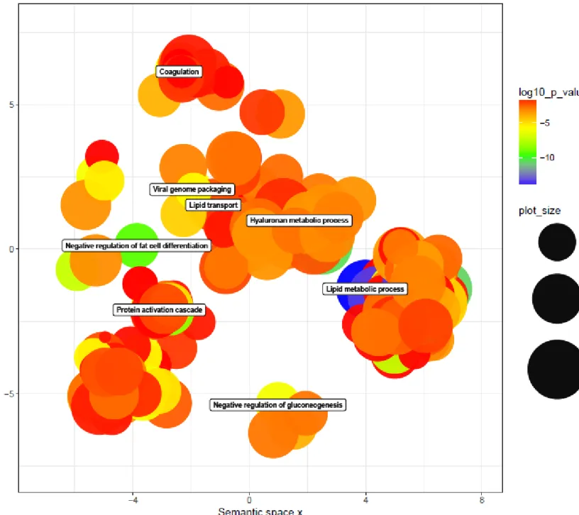
Table 3.10: List of the top most significant 10 annotated tissue-specific genes of each tissue with the gene ID from UniProtKB and the respective protein name and FDR. 28 Table 3.11: Summary of orthologues of the MFAP4 gene (Figure adapted from http://Oct2018.archive.ensembl.org/Bos_taurus/Gene/Compara_Ortholog?db=core;g=ENSBT AG00000006187;r=19:34685357-34687892;t=ENSBTAT00000008130). 33 Table 3.12: Top 10 gene ontologies according to their dispensability thoughout the studied tissues with their respective GO identifications, descpription and log10 p-values. 52 Table 6.1: Top 10 gene ontologies according to their dispensability thoughout the studied tissues with their respective GO identifications, descpription and log10 p-values. 79

X Figure 1.1: Strategies for reconstructing transcripts from RNA-Seq reads [1]. 5

Figure 1.2: Overview of Trinity [2]. 6

Figure 1.3: Sardine historical landings (line) and biomass (columns) [3]. 8 Figure 1.4: Main phylogenetic hypothesis of bony fish groups collapsed to depict higher-level

clades [4]. 10

Figure 2.1: Flowchart of the methodology. The original reads go through a quality control check, followed by the assembly with Trinity and another quality control step with Transrate and finnaly annotated with Trinotate that uses various search tools for protein and transcript

analyses in different databases. 13

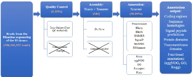
Figure 3.1: Methodology decision making flowchart and respective results. The original 593,341,322 reads went through a quality control check using Trim Galore and Trimmomatic which were compared with FastQC. The results from Trim Galore, with an average of 0.35% reads removed, proceded to the assembly with Trinity by de novo and genome guided. The results from the de novo assembly plus Transrate proceed to the annotation with Trinotate. N50 and SwissProt annotation results of the caudal fin de novo assembly were 540 and 38.01%, respectively. The results for all assemblies and respective annotations are described in tables

3.5, 3.6, 3.7 and 3.8. 18

Figure 3.2: Trinity Transcript Quantification. Filtered to show up to 100 TPM. Linear regression

between 10 TPM to 100 TPM in blue, 10 TPM in red. 27

Figure 3.3: MFAP4 gene gain/loss tree. This gene family has significant gene gain or loss events (p-value for the gene family is 0, as computed by CAFE). *Clupeocephala node. (Figure

adapted from

http://oct2018.archive.ensembl.org/Bos_taurus/Gene/SpeciesTree?db=core;g=ENSBTAG000 00006187;r=19:34685357-34687892;t=ENSBTAT00000008130). 34 Figure 3.4: MYH7 gene gain/loss tree. This gene family does not have any significant gene gain or loss events (p-value for the gene family is 0.692, as computed by CAFE). *Clupeocephala

node. (Figure adapted from

http://oct2018.archive.ensembl.org/Equus_caballus/Gene/SpeciesTree?db=core;g=ENSECAG

00000019844;r=1:161506573-161527244) 36

Figure 3.5: PPN gene gain/loss tree. This gene family does not have any significant gene gain or loss events (p-value for the gene family is 0.995, as computed by CAFE). *Clupeocephala

node. (Figure adapted from

http://oct2018.archive.ensembl.org/Mus_musculus/Gene/SpeciesTree?family=PTHR13723_S

XI Figure 3.6: Heatmap of the correlation of the different tissues. (Colour represents the value of similarity with purple representing the least similarity and yellow the most. Tissues were clustered according to their similarity and the white muscle tissue was the considered outlier. Abbreviations of the tissues are extended on the list of abbreviations) 38 Figure 3.7: Heatmap of tissue-specific genes predicted in different tissues. (Colour represents the value of expression on each tissue with purple representing the least expression and yellow the most. Tissues and genes were clustered according to their expression pattern similarities. Abbreviations of the tissues are extended on the list of abbreviations) 39 Figure 3.8: Gene ontology scatterplot generated with REVIGO for the gill plus branchial arch

tissue. 41

Figure 3.9: Gene ontology scatterplot generated with REVIGO for the liver tissue. 42 Figure 3.10: Gene ontology scatterplot generated with REVIGO for the spleen tissue. 43 Figure 3.11: Gene ontology scatterplot generated with REVIGO for the gonad tissue. 44 Figure 3.12: Gene ontology scatterplot generated with REVIGO for the midgut tissue. 45 Figure 3.13: Gene ontology scatterplot generated with REVIGO for the white muscle tissue.

46 Figure 3.14: Gene ontology scatterplot generated with REVIGO for the red muscle tissue. 47 Figure 3.15: Gene ontology scatterplot generated with REVIGO for the kidney tissue. 48 Figure 3.16: Gene ontology scatterplot generated with REVIGO for the head kidney tissue.

49 Figure 3.17: Gene ontology scatterplot generated with REVIGO for the brain plus pituitary

tissue. 50

Figure 3.18: Gene ontology scatterplot generated with REVIGO for the caudal fin tissue. 51 Figure 6.1: Per base sequence quality of gill plus branchial arch reads. 62 Figure 6.2: Per base sequence quality of liver reads. 62 Figure 6.3: Per base sequence quality of spleen reads. 63 Figure 6.4: Per base sequence quality of gonad arch reads. 63 Figure 6.5: Per base sequence quality of midgut reads. 64 Figure 6.6: Per base sequence quality of white muscle reads. 64 Figure 6.7: Per base sequence quality of red muscle reads. 65 Figure 6.8: Per base sequence quality of kidney reads. 65 Figure 6.9: Per base sequence quality of head kidney reads. 66 Figure 6.10: Per base sequence quality of brain plus pituitary reads. 66 Figure 6.11: Per base sequence quality of caudal fin reads. 67

XII Figure 6.12: Gene ontology scatterplot generated with REVIGO for the gill plus branchial arch

tissue. 68

Figure 6.13: Gene ontology scatterplot generated with REVIGO for the liver tissue. 69 Figure 6.14: Gene ontology scatterplot generated with REVIGO for the spleen tissue. 70 Figure 6.15: Gene ontology scatterplot generated with REVIGO for the gonad tissue. 71 Figure 6.16: Gene ontology scatterplot generated with REVIGO for the midgut tissue. 72 Figure 6.17: Gene ontology scatterplot generated with REVIGO for the white muscle tissue.

73 Figure 6.18: Gene ontology scatterplot generated with REVIGO for the red muscle tissue. 74 Figure 6.19: Gene ontology scatterplot generated with REVIGO for the kidney tissue. 75 Figure 6.20: Gene ontology scatterplot generated with REVIGO for the head kidney tissue.

76 Figure 6.21: Gene ontology scatterplot generated with REVIGO for the brain plus pituitary

tissue. 77

1

1 Introduction

Biotechnology is defined as the exploitation of biological systems, living organisms, or their derivatives in technological applications to make or modify products or processes generally for societal benefit [5]. To engage with the public and to have an easy to understand system, biotechnology can be divided into colour codes. White biotechnology is related to industrial processes, red biotechnology is related to medical processes, green biotechnology is related to agricultural processes and blue biotechnology is related to marine and aquatic processes. In this project, the organism in question is a fish therefore the present project fits within blue biotechnology, which includes marine aquaculture and ocean farming. The present project is focused on the assembly and annotation of the European sardine (Sardina pilchardus) or sardine transcriptome and the project will form the basis of future studies.

The transcriptome is derived from an organism’s DNA and contains the information necessary for all the proteins required to build and sustain an organism. Transcriptomics provides a wealth of information that can be used for a diversity of possible studies on a given organism. But in order to study the transcriptome the first thing that needs to be done is to sequence it. Recent development in sequencing, or Next Generation Sequencing (NGS) methods are leading to an unprecedented increase in available transcriptomes and underpins the remarkable big data results. To manage this big data, it is essential to have access to bioinformatic tools supported by high computing processes and much of this thesis will be based on the application of bioinformatics to assemble and analyse the transcriptomes generated from a number of sardine tissues.

The sardine is the target species because of it elevated economic and cultural importance for the Mediterranean and due to an unexplained and unexpected decline in the stock there are several species conservation concerns. Relatively few molecular resources are available for the sardine, which is a non-model organism and the factors underlying the population decline are unknown. The availability of molecular resources for the sardine is a priority as it will be a tool that will enable studies of biotic factors that may explain the population decline. The present project aims to assemble and annotate the transcriptome of the sardine and in this way, increase the molecular (both genomic and transcriptome) data for studies of this species.

2

1.1 Transcriptome

An organism’s entire biological information is coded in its genome, which consists of DNA that gains structure in the chromosomes through its interaction with histones and other molecules [6]. Through the process of transcription, DNA is copied into RNA with the help of RNA polymerases, helicases and transcription factors. RNA polymerase binds to a sequence of DNA located before what is going to be expressed called the promoter and starts building an RNA strand, complementary to the DNA, which will serve as the template for the other RNA strand, while helicase is responsible for breaking the hydrogen bonds of DNA, separating the two strands. In turn, the RNA gets translated into proteins that are frequently important in modulating or determining the phenotype of an organism [7]. The transcriptome is most simply defined for any specific stage of every physiological condition as every RNA molecule in a cell or tissue, and the quantity. Transcriptomics aims to catalogue all the transcripts, including mRNAs, non-coding RNAs and small RNAs, determine the transcriptional structure of genes and to quantify the expression levels of each transcript. To extract total RNA, it is necessary to take into consideration that RNA molecules are very labile and degrade rapidly over time so the quality of the RNA being used for transcriptomics needs to be checked. In most cases to analyse expression data, the RNA coding information is passed into a more stable molecule (cDNA) via reverse transcription. In the RNA-seq wet lab process the RNA coding information is passed into cDNA during the RNA-seq sequencing library construction [6].

1.2 Sequencing

There are a number of different types of biological sequences, but the present study is most directed at the nucleic acid and proteomic sequences. DNA nucleotide sequences differ from RNA since the base thymine is substituted by uracil and the sugar in the nucleotide in DNA is deoxyribose and in RNA is ribose. Sequencing provides information about the sequence of bases or amino acids in a nucleic acid or protein, respectively and thus yields the primary structure of the sequence (Mardis 2008).

Sequencing of nucleic acids started with the Sanger method. Sanger sequencing consists in running four reactions in parallel, one for each of the bases, and generating one long sequence at a time. The sequencing reaction ends with a radioactively or fluorescent labelled dideoxy nucleotide. Analysing the size of the fragments originated from the sequencing reaction allows the order of the bases in a sequence to be established. The advance of technology means that Sanger sequencing has been replaced by Next Generation Sequencing (NGS) [9]. NGS

3 techniques are based on massive parallel sequencing where millions of small fragments of DNA are simultaneously amplified. Most techniques emit some kind of signal that represents and indicates a base has been added. Different techniques vary in relation to the signal produced or the sequencing reaction itself [8]. The signal is captured by a computer that saves the information as RNA-seq data.

While NGS is the most recent method it is still sometimes preferable to use the Sanger method due to its cost effectiveness. The Sanger method is best used to sequence up to 100 fragments with a higher accuracy and lower cost than NGS. The actual NGS RNA-seq output comes in the format of FastQ files, structured in four text lines per read, the first consists of the name of the read, the second the read’s nucleotide base sequence and in the fourth their respective base qualities in Phred33 coding, a code in each character, there is a quality value assigned to it [10]. Handling these big files is a challenge and requires high throughput processing computers and bioinformatics knowhow in the Unix environment. The reason Unix is preferred is due to the powerful use of its tools that allow big file editing and the ability to connect to servers where the commands can be run.

1.3 Bioinformatics

The application of tools of computation and analyses to capture and interpret biological data is the core of Bioinformatics. This approach uses sophisticated software, pipelines and platforms connected through the internet or machines to build genomes and transcriptomes.

The advance of technologies in Genomics led to an era in the early 90’s of “Large Data

Acquisition” where biological data kept accumulating at a fast pace and there was a need to deal

with the high amounts. As more data is accumulated and stored we have now entered the “Big

Data era”. With the continuous evolution of high throughput methods the challenge is now how

to compute the data and efficiently store, transfer, secure and process the large amounts of data, while minimising the errors [11], [12].

Different types of data in bioinformatics can be defined, the main five are: gene expression (transcriptome study); DNA, RNA and protein sequence; protein-protein interaction; pathway; gene ontology [13]. For a transcriptome study identifying novel transcripts from annotated genes, splicing isoforms and gene-fusion transcripts is fundamental. Three major steps are required for transcriptome studies, these steps can be performed with different tools depending on factors like the sequencing technique used, the type of organism in study and the goal of the analyses but consist on the same general principles. Data pre-processing is required to remove

4 sequencing adaptors, insertions resulting from library preparation and near-identical reads to correct sequencing errors and improve the read quality. A transcriptome assembly strategy can be reference-based (using the genome sequence as the reference), de novo assembled or a combination of both [14]. Once assembled a range of tools are available to search for sequence similarities using various public databases, such as Swiss-Prot, Pfam, eggNOG (evolutionary genealogy of genes: Non-supervised Orthologous Groups), GO (Gene Ontology) and Kegg (Kyoto enciclopedia of genes and genomes), to analyse the contigs from the assembled transcriptome and annotate them.

The three main methodological steps in the present project were, 1) processing of the raw read quality, 2) the assembly of the sequence reads and 3) the annotation.

Quality control methodology

Quality control tools are required to assess and edit raw sequence read data, as adapter contaminations and low-quality bases can pose a real problem depending on the library preparation and downstream application. Two approaches will be tested in the thesis project to consistently apply quality and adapter trimming to FastQ files, first the Trim Galore software (www.bioinformatics.babraham.ac.uk/projects/trim_galore/), and secondly the Trimmomatic (github.com/timflutre/trimmomatic) plus FastQC. Trim Galore is a wrapper tool around Cutadapt and FastQC. Cutadapt (github.com/marcelm/cutadapt/) finds and removes adapter sequences, primers, poly-A tails and other types of unwanted sequence from high-throughput sequencing reads. FastQC (www.bioinformatics.babraham.ac.uk/projects/fastqc/) is a quality control tool for high throughput sequence data producing an overall report of the edited reads. FastQC is also used in the second approach to confirm the edited output of Trimmomatic. Trimmomatic is a fast, multithreaded command line tool that can be used to trim and crop Illumina (FASTQ) data as well as to remove adapters and is similar to the program Cutadapt.

Assembly methodology

Assembly tools process large volumes of RNA-seq reads, the assembly procedures may be different depending on the software and whether or not there is prior genomic reference data. If there is a reference genome available it can be genome-guided, where the reads are first aligned to the genome, if there isn’t a genome it must be a de novo assembly procedure and reads are assembled when they overlap each other, it is also possible to use a combination of the methods. Various software are freely available including Oases, Trinity, trans-ABySS and Cufflinks.

5

Figure 1.1: Strategies for reconstructing transcripts from RNA-Seq reads [1].

In the present thesis the software used for assembly was Trinity (github.com/trinityrnaseq/trinityrnaseq/wiki) (Grabherr, M. et all 2013), an efficient and robust

de novo reconstruction of transcriptomes from RNA-seq data and also more recently a genome

guided reconstruction. Trinity combines three independent software modules: Inchworm, Chrysalis, and Butterfly. Inchworm assembles the RNA-seq data into the unique potential sequence as contigs resulting from the kmers extensions combinations, Chrysalis clusters the Inchworm contigs into clusters when they overlap and constructs complete de Bruijn graphs for each cluster, and finally Butterfly then processes the individual graphs in parallel, tracing the paths that reads and pairs of reads taken within the graph, ultimately reporting full-length transcripts for alternatively spliced isoforms, and separating transcripts that corresponds to paralogous genes (Figure 1.2). Bowtie2 (bowtie-bio.sourceforge.net/bowtie2/index.shtml) is an ultrafast and memory-efficient tool for aligning sequencing reads to long reference sequences and is used in the present project to allow genome guided transcriptome assembly. Two approaches will be tested, Trinity de novo and Trinity genome guided assemblies. The metrics

6 of the assemblies generated will be compared to decide which output generated will be annotated. Before the annotation, a post-assembly quality control is implemented using Transrate (http://hibberdlab.com/transrate/) [16], a software for transcriptome assembly quality analysis.

7

Annotation methodology

Annotation is the next step after assembly and consists of identifying assembled transcripts by comparison with other transcripts in public databases and assigning their function based on the most similar transcripts found, whether it belongs to the same species or not, considering their primary structure, corresponding proteins and domains. This makes it possible to separate putative proteins based on their involvement in cellular components, biological processes and molecular functions.

Annotation tools identify coding sequences by similarity and composition searches in databases. There are many automated pipelines created for this purpose such as Annocript, Trinotate, Blast2GO and TRAPID that go through different databases. In the present study Trinotate (trinotate.github.io/) - comprehensive annotation suite designed for automatic functional annotation of transcriptomes, particularly de novo assembled transcriptomes, from model or non-model organisms was used. Trinotate makes use of a number of different well referenced methods for functional annotation including homology searches to known sequence data (BLAST+/SwissProt), protein domain identification (HMMER/PFAM), protein signal peptide and transmembrane domain prediction (signalP/tmHMM), and also leverages various annotation databases (eggNOG/GO/Kegg databases). All functional annotation data derived from the analysis of transcripts is integrated into a SQLite database which allows fast efficient searching for terms with specific qualities related to a desired scientific hypothesis or as a means to create a whole annotation report for a transcriptome.

1.4 Sardine

The sardine (Sardina pilhardus) is a subtropical small pelagic fish distributed along the north-eastern Atlantic Ocean and in the Mediterranean Sea belonging to the Clupeidae family. It is the most important fish in terms of catch biomass with the biggest fishery occurring in Morocco [17]. Catches of the sardine have been increasing over the past years, in 1960, 487 900 tons were captured and in 2010 the total capture for the sardine has risen to 1 245 956 tons 2010 (FAO 2017). Fish stock management studies indicate that the capture of sardine is no longer sustainable and to avoid the collapse of the stocks the European community has lowered the allowable catch and in Portugal the volume of landings for this fishery has rapidly decreased. This has led to considerable problems within the sector and has changed the sardine from a “poor mans” food as market prices have soared from 1-2 euros/kg to 8-10 euros/kg. As a consequence of this decline in the available sardine biomass in Portuguese waters there has

8 been a rise in interest in establishing why the stock has collapsed. Concern has been raised in relation to the conservation of the sardine. Some fishermen take this concern seriously while others think there is no danger to the population (H. O. Braga et al. 2017). Recent studies found that the biomass of the sardine is currently declining along with its harvest, however the reason for the decline in the population isn’t clearly known.

Figure 1.3: Sardine historical landings (line) and biomass (columns) [3].

Sardine biology and ecology

Sardines have grey subcylindrical bodies with a rounded belly and dark spots, the last 2 anal fin rays are enlarged and grow up to 25 cm. The sardine is a serial spawner and starts breeding at one year old throughout the year, mostly in the winter, near the shore and it has a maximum reported life span of 15 years, reaching maturity at 1 year old when it is around 8 cm and it swims in large schools. The sardine mostly eats planktonic crustaceous and occupy a basal position on the food chain, transferring energy from plankton and small organisms to larger fishes, sea birds and marine mammals with great influence over the health of the animals above the sardine in the food chain (Jawad 2015, FAO 2017). Females tend to be slightly larger, heavier and less abundant than males and sardines from offshore tend to be bigger than those that are inshore [21], [22]. They are also of interest due to some distinct biological characteristics they possess such as rapid growth and resistance to algal blooms.

9

Rationale for transcriptome characterization

The decrease in the sardine population is a recent debated concern and the difficulties in its conservation can possibly have a negative consequence in the ecosystem. To know what changes this may cause and maybe spread awareness there needs to be more studies. Since there isn’t much information available on this specific fish because it isn’t a model organism, one starting point is to characterize its transcriptome and then annotate the transcripts. The long-term final objective is to delong-termine the population structure and dynamics and separate them based on biological borders and not geopolitical.

On the NCBI website there are 57.196 entries on the nucleotide database of Expressed Sequence Tags and Genome Survey Sequences for all the clupeiformes and most of the reads (39,344) are for Clupea harengus (Atlantic herring) and only 566 are for Sardina pilchardus and the latter sequences are mainly cytochrome related (NCBI December 2017). During the current project, the sardine’s genome was assembled and reported in a manuscript entitled “A haplotype-resolved draft genome of the European sardine (Sardina pilchardus)” (http://bioinformatics.psb.ugent.be/orcae/overview/Spil, Genebank Bioproject PRJEB26757 ) [23]. The information generated in this project may contribute to studies trying to establish the unique characteristics of the sardine by comparing its transcriptome with other closely related vertebrate fishes and help better understand evolution since the sardine belongs to the clupeiformes order which is situated in an older position in the phylogenetic tree relative to other orders with more studied fishes that went through more recent speciation events (Figure 1.4).

10

Figure 1.4: Main phylogenetic hypothesis of bony fish groups collapsed to depict higher-level

11

1.5 Objective

This project intends to develop a representative transcriptome for the adult sardine with the help of bioinformatic tools to serve as a resource for future biological and genetics studies of the sardine, which is a non-model organism, that benefit from, or require looking at its transcriptome. This is achievable by using sequencing data for several tissues and executing a series of algorithms that go through important stages to get the most accurate transcriptome as possible and will be run in servers with high performance computing. Different bioinformatics methodologies will also be approached for the transcriptome analysis. The different stages will serve to:

• Trim the reads and exclude the small and poor-quality reads using 2 different tools. • Assemble the resulting reads into a mapped transcriptome using 2 different ways; • Annotate the possible genes by comparing them with transcripts of other species in data bases.

2 Material and Methods

The methodology of the bioinformatic workflow applied in this study is represented in figure 2.1.

2.1 Sampling

Eleven tissues were collected from a single female sardine, blood was also sampled for the purpose of genome sequencing. The female was fished off the shore from Olhão, on May 2016 and maintained in Pilot Station of Aquaculture in Olhão (EPPO) until it was sacrificed by an overdose of anaesthesia (1:250, 2-phenoxyethanol) followed by euthanasia by cervical section in September 2017. The tissues were then preserved in RNAlater® and stored at -20 ºC. In the context of the genome sequencing project in which the transcriptome is integrated, a bioproject (PRJEB27990) has been created in the European Nucleotide Archive (ENA) where the samples have the accession numbers listed in table 2.1.

12

Table 2.1: List of the tissues used as a source of RNArespective abbreviations and sample accession number in ENA archive.

Tissue Abbreviation Sample Accession

Gill + Branchial Arch Gi SAMEA4809353

Liver Lv SAMEA4809357

Spleen Sp SAMEA4809360

Gonad (female) Gn SAMEA4809354

Midgut Mg SAMEA4809358

White Muscle WM SAMEA4809350

Red Muscle RM SAMEA4809359

Kidney Kd SAMEA4809356

Head Kidney HKd SAMEA4809355

Brain + Pituitary Br SAMEA4809351

Caudal Fin (Skin + Cartilage + Bone) CF SAMEA4809352

2.2 Sequencing

The total RNA from the eleven tissues was extracted using a Maxwell® 16 Total RNA Purification Kit after they were mechanically disrupted. Total RNA was then double-treated using a DNA-free kit with DNase, quantified by NanoDrop 1000 Spectrophotometer and stored at -80 ºC as described in the genome manuscript “A haplotype-resolved draft genome of the European sardine (Sardina pilchardus)”[23].

The mRNA was isolated from the total RNA using a NEBNext® Poly(A) mRNA Magnetic Isolation Module kit and sequenced using Illumina – HiSeq4000 PE 150 bp Cycle with the NEBNext® Ultra™ Directional RNA Library Prep kit. The quality control of the mRNA was made with Qubit, Tapestation and the quality was above 8 RIN. This part was done by the Admera Health company and generated stranded paired-end reads. The adapters used for the sequencing and considered in the quality control procedures for the removal of these sequences from the resulting reads by the software were the following:

13

Table 2.2: Illumina sequencing adapters used in the sequencing. R1 and R2 are forward and

reverse reads, respectively of the paired-end reads. Sequence orientation 5’ to 3’.

Read Adapter Sequence Reverse complement

R1 AGATCGGAAGAGCACACGTCTGAACTCCAGTCA TGACTGGAGTTCAGACGTGTGCTCTTCCGATCT

R2 AGATCGGAAGAGCGTCGTGTAGGGAAAGAGTGT ACACTCTTTCCCTACACGACGCTCTTCCGATCT

2.3 Computational usage

Most algorithms ran on the “High Performance Computing” (HPC) of INCD (Infraestrutura Nacional de Computação Distribuída) servers located in Lisbon through the Unix environment. Processes that demanded high memory to run were queued with qsub that orderly runs batch job submissions in different parted machines (Examples of the codes and R scripts used in appendices 6.1).

Figure 2.1: Flowchart of the methodology. The original reads go through a quality control

check, followed by the assembly with Trinity and another quality control step with Transrate and finnaly annotated with Trinotate that uses various search tools for protein and transcript analyses in different databases.

14

2.4 Quality Control and Reads Editing

The quality control and reads trimming were performed with two alternative software pipelines: Trim Galore version 0.4.5 and Trimmomatic version 0.36 plus FastQC version 0.10.1, for methodological comparative purposes.

2.4.1 Trim Galore

With Trim Galore, a wrapper of Cutadapt and FastQC, the code used had parameters to trim quality ends from reads if the score was below 20 (default), indicate to use ASCII+33 quality scores as Phred scores, remove 1 bp from the 5’ end of read 1 and 2, a stringency of 3 bp overlapping with adapter sequence required to trim a sequence, allow a maximum error rate of 0.1 (default). After Cutadapt trimmed the reads, it discarded reads that became shorter than 30 bp and unpaired reads and the output was edited FastQ files compressed with gzip. Edited reads were then analysed by FastQC to generate the quality report with descriptive statistics represented in a graphical format for better decision making of subsequent procedures.

2.4.2 Trimmomatic plus FastQC

The Trimmomatic command used had parameters to specify the input type as paired-end reads, use 4 threads, trim reads if the average quality of a window across 4 bases was below 20, keep reads of a minimum of 30 bp, find and remove Illumina adapters specified in the “adapter.fa” file with a maximum of 2 mismatches and remove 1 base from the start of the read. Edited reads were also analysed by FastQC downstream to visualize the quality of the output the same way as with Trim Galore.

2.5 Assembly

The transcriptome assembly was achieved with Trinity version 2.5. A post assembly quality control step was made using Transrate version 1.0.3 by comparing the assemblies with the raw reads. Transrate ran only for the assemblies generated with the De Novo approach. Assemblies were generated for each tissue and an additional assembly containing the reads from all the tissues.

15

2.5.1 De Novo assembly

The Trinity command used for de novo assembly had parameters to indicate the reads were in FASTQ format, had a maximum memory usage of 184G of RAM, 8 CPU and the orientation of R1 and R2 were the reverse forward read, respectively. Additional parameters specified were minimum contig length of 200 bp (default) and run normalization separately for each pair of FASTQ files, then one final normalization that combined the individual normalized reads with a maximum read coverage of 50 (default). To obtain the metric statistics of the assemblies a script (TrinityStats.pl) provided by Trinity was run.

The code for Transrate had parameters to use 8 threads (default) and to indicate the left and right reads in FASTQ format in addition to the assembly input in FASTA format.

2.5.2 Genome Guided

Before the genome guided assembly could be run, an alignment of the RNA reads against the genome sequence was required, this alignment was made with Bowtie2 (version 2.3.4) which forms output in the form of a Sequence Alignment Map (SAM) file. This alignment procedure had two alternatives approaches, one that makes local alignments and the other that performs end-to-end alignments, so both were tested. The parameters of Bowtie2 specified in the command were that the reads were in FASTQ format, the orientation of R1 was Reverse and the orientation of R2 was Forward, and to use 14 CPU. The parameters specified for the input data were all RNA FastQ files from the present study and the preliminary draft genome assembly of the sardine. After the alignment, a pipeline of Samtools (version 1.1) utilities converted the SAM files to Binary Alignment Map (BAM) files with the command view and then sorted them with the command sort.

The trinity genome guided command uses solely the sorted BAM to retrieve sequence information for the assembly, the specified parameters to indicate a maximum intron length of 10,000 bp (for the end-to-end alignment based) and 25,000 bp (for the local alignment based), a maximum memory of 114G of RAM and to use 14 CPU were used.

To get the metric statistics of the assemblies generated a script “TrinityStats.pl” provided by Trinity was ran on both assemblies FASTA files.

16

2.6 Functional Annotation

The functional annotation of the transcriptome assemblies obtained was done using the Trinotate version 3.1.1 annotation pipeline, and the REVIGO (revigo.irb.hr/) [24], a web server that summarizes long, unintelligible lists of GO terms by finding a representative subset of the terms using a simple clustering algorithm that relies on semantic similarity measures. Software’s required for the Trinotate pipeline included TransDecoder (5.0.2), SQLite (3.6.20), NCBI BLAST+ (2.7.1), HMMER (3.1 and 2.3 for the RNAMER), tmHMM (2.0), SignalP (1.05, with Perl (5.8.8)) and RNAMMER (1.2).

2.6.1 Trinotate

The obtained deduced proteins FASTA file “transdecoder.pep” was used as input for several annotation programs that belong to the Trinotate pipeline; the “SignalP” to predict signal peptides, the “tmHMM” to predict transmembrane regions, the “HMMER” (hmmscan) to identify protein domains of the PFAM v30.0 database (“Pfam-A.hmm”, 15th _{Feb 2018)}

Blastp to identify protein homologies of Swissprot/Uniprot database (accessed 14th Feb 2018). The transcriptome nucleotide FASTA file “good.trinity.fasta” was used as input for ribosomal RNA using RNAMER program and query the same Swissprot/Uniprot database but using blastx.

All output of the several annotation analysis was then integrated into single SQLlite database already populated with GO, eggNOG, and KEGG pathways via the Trinotate utility.

This procedure as done to all transcriptomes curated by Transrate, for comparison purposes two Transrate non-curated transcriptomes (Caudal Fin and all tissues) were also annotated following the same procedure.

2.6.2 Transcript Quantification

To count the overall transcripts being expressed, several Trinity scripts were used with the assembly of the reads from all the tissues after going through Transrate. Firstly, the “align and estimate abundances.pt” script aligned and estimated abundances and had parameters to indicate the input as a FASTA file, paired-end, the use of the RSEM method and the use of the bowtie2 alignment method. Secondly, the “abundance_estimates_to_matrix.pl” script used the estimates to create matrices of counts and of normalized expression values and had parameters

to the use of the RSEM method. Thirdly, the

“count_matrix_features_given_MIN_TPM_threshold.pl” script counted the expression numbers on the matrices. Finally, using R language, a linear regression was calculated and

17 plotted, within the range of 10-100 TPM to obtain the intersect representing the total count of genes being expressed. an Rplot was edited to provide the graphs for total gene and transcript expression.

2.6.3 Tissue-specific genes

For the prediction of the specific genes from each tissue with a threshold of 95% of total expression, normalised counts matrix of each tissue vs the all the others were created with a Trinity Differential Expression script “run_DE_analysis.pl” specifying the parameters of 0.4 dispersion and the use of RSEM method. A heatmap for the predicted tissue-specific genes was generated using the Trinity Differential Expression scripts “analyse_diff_expr.pl” using the Transrate non-curated all tissues assembly.

2.6.4 REVIGO

GO enrichment analysis were performed with GOseq scripts, the first from Trinotate toolkit and the others from Trinity. “extract_GO_assignment_from_Trinotate_xls.pl” created a file with the GO annotations, “fasta_seq_lenght-pl” created a file with the transcript lengths with the use of the transcript lengths, “TPM_weighted_gene_lenght.py” created a file with the gene lengths, and finally, “run_GOseq.pl” created files with enriched and depleted categories. The resulting list of GO terms with their associated over representative p-values was used for REVIGO analysis with an allowed similarity of 0.9, 0.7 and 0.5 for biological process and molecular function. The scatterplot based on REVIGO semantic similarity results were plotted using R language. This procedure was done for all assemblies.

18

3 Results and Discussion

The results of each section of the project determined which method was adopted before moving onto the next pipeline step as detailed in figure 3.1.

Figure 3.1: Methodology decision making flowchart and respective results. The original

593,341,322 reads went through a quality control check using Trim Galore and Trimmomatic which were compared with FastQC. The results from Trim Galore, with an average of 0.35% reads removed, proceded to the assembly with Trinity by de novo and genome guided. The results from the de novo assembly plus Transrate proceed to the annotation with Trinotate. N50 and SwissProt annotation results of the caudal fin de novo assembly were 540 and 38.01%, respectively. The results for all assemblies and respective annotations are described in tables 3.5, 3.6, 3.7 and 3.8.

3.1 Quality Control and Reads Editing

The sequencing of the 11 tissues generated in total about 600 million (593,341,322) paired-end reads that were submitted to the ENA archive under the accession run numbers from ERR2720641 to ERR2720651, that had to be trimmed for better quality.

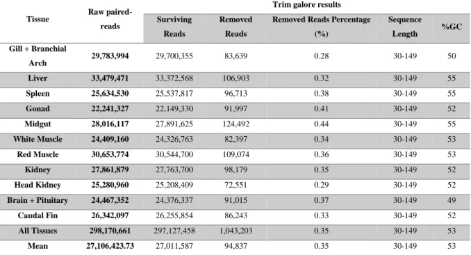
Two approaches were compared for the quality control and reads editing. The parameters used for both the Trim Galore and the Trimmomatic were as similar as possible to better compare them without different variables. The indication of Illumina adapters wasn’t needed for Trim Galore as it recognized them automatically. Reads and the respective pair were discarded if they were less than 30 bp in length. Quality editing of the reads is essential for the assembly procedures, as adapter contaminations and low-quality reads lead to poor assembly’s outcomes with many artefacts that can prevent the assembler software from being able to deal with data. Results from the Trim Galore gave reads above 28 quality score (Figures in appendices 6.2) from 30 to 149 bp, GC percentages from 49 to 55 % in line with coding sequences/GC richer relationship and removed from 0.28 to 0.44 % of the original reads sequences.

19

Table 3.1: Trim Galore edited results of the raw paired-reads from the 11 sequenced sardine

tissue libraries.

Results from the Trimmomatic granted reads above 32 quality score from 1 to 149 bp and GC percentages from 49 to 55 % and removed from 5.77 to 8.08 % of the original sequences.

Table 3.2: Trimmomatic edited results of the raw paired-reads from the 11 sequenced sardine

tissue libraries.

Tissue Raw paired-reads Trimmomatic results Surviving Reads Removed Reads

Removed Reads Percentage (%) Sequence Length %GC Gill + Branchial Arch 29,783,994 28,065,613 1,718,381 5.77 1-149 50 Liver 33,479,471 31,305,340 2,174,131 6.49 1-149 55 Spleen 25,634,530 23,690,270 1,944,260 7.58 1-149 55 Gonad 22,241,327 20,482,936 1,758,391 7.91 2-149 52 Midgut 28,016,117 25,757,615 2,258,502 8.06 2-149 55 White Muscle 24,409,160 22,446,925 1,962,235 8.04 3-149 53 Red Muscle 30,653,774 28,176,295 2,477,479 8.08 2-149 53 Kidney 27,861,879 25,767,818 2,094,061 7.52 4-149 52 Head Kidney 25,280,960 23,522,879 1,758,081 6.95 2-149 52 Brain + Pituitary 24,467,352 22,734,872 1,732,480 7.08 1-149 49 Caudal Fin 26,342,097 24,648,080 1,694,017 6.43 1-149 52 All Tissues 298,170,661 276,598,643 21,572,018 7.23 1-149 53 Mean 27,106,423 25,145,331 1,961,092 7.23 2-149 53

Tissue Raw paired-reads

Trim galore results Surviving

Reads

Removed Reads

Removed Reads Percentage (%) Sequence Length %GC Gill + Branchial Arch 29,783,994 29,700,355 83,639 0.28 30-149 50 Liver 33,479,471 33,372,568 106,903 0.32 30-149 55 Spleen 25,634,530 25,537,817 96,713 0.38 30-149 55 Gonad 22,241,327 22,149,330 91,997 0.41 30-149 52 Midgut 28,016,117 27,891,625 124,492 0.44 30-149 55 White Muscle 24,409,160 24,326,763 82,397 0.34 30-149 53 Red Muscle 30,653,774 30,544,700 109,074 0.36 30-149 53 Kidney 27,861,879 27,763,700 98,179 0.35 30-149 52 Head Kidney 25,280,960 25,208,409 72,551 0.29 30-149 52 Brain + Pituitary 24,467,352 24,376,337 91,015 0.37 30-149 49 Caudal Fin 26,342,097 26,255,854 86,243 0.33 30-149 52 All Tissues 298,170,661 297,127,458 1,043,203 0.35 30-149 53 Mean 27,106,423.73 27,011,587 94,837 0.35 30-149 53

20 Trimmomatic results revealed that it removed more sequences than CutAdapt from Trim Galore, a difference of overall 6.88 % as it considered more reads to be of low quality, and yielded reads smaller than 30 bp in discordance with the size threshold defined in the Trimmomatic command. The GC percentage of the surviving reads were the same for both assembly approaches, around 53 %, which seems to be appropriated to gene expression products (Tables 3.1 and 3.2).

Results from Trimmomatic granted a per base sequence quality slightly higher than Trim Galore (Figures in appendices 6.2). Every other aspect of the assemblies remained very similar or equal. Ordering the tissues by their removed reads percentages yielded similar lists and the gill plus branchial arch tissue was always the tissue with the lower removed reads percentages in both approaches.

To proceed to the assembly, the output of the Trim Galore was chosen because of the unpredicted behaviour of Trimmomatic with regards to retaining reads smaller than 30 bp, and the higher than expected ratio of low quality reads removal, even though Trimmomatic showed slightly better quality scores.

3.2 Assembly

Two approaches were compared for the assembly. The Trinity de novo and Trinity genome guided assemblies that could be done with either local or end-to-end alignments. Besides assembling the reads from each tissue, a reference assembly was made using the reads from the 11 tissues for a global analysis. Of the many statistics obtained, the ones considered more relevant were the GC-content, mean length of sequence, number of contigs assembled and N50. A higher N50 and mean length values meant there was a higher chance of the assembly being less fragmentated and more likely to cover the genes full coding region in an ideal scenario. However N50 might not be completely accurate as artefacts such as contigs concatemerizations might and wrongly generated longer contigs lead to biased inflated N50´s values, due to very similar genomic regions of duplicated genes. Since the teleosts have gone through 3 whole genome duplication events there is high probability of existing very similar sequence regions, for example from paralogous genes and DNA copy number variations, that could be assembled in the same contig [25], [26]. These artefact contigs lead to a higher N50 that does not necessary mean that it belongs to a better assembly.

The assembly from the reads of all the tissues after Transrate was used in modelling the gene predictions for the genome annotation project, improving the detection of genomic features such as untranslated regions and organism specific genes[27]. The RNA-seq assembly,

21 repetitive elements and protein homology and ad initio gene prediction were used as inputs for the software’s MAKER and SNAP (Semi-HMM-based Nucleic Acid Parser) to generate the gene models. For validation and assessment of genome completeness, the RNA-seq reads should have a high alignment rate with the genome as this indicates a good quality assembly, in these study all raw reads aligned with 90 % of the sardine draft genome (data not shown) indicating a good genomic assembly.

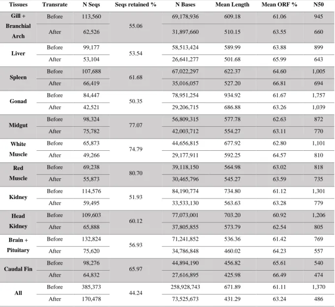
After Transrate assembly curation, 44 to 80 % contigs were retained from the initial Trinity de

novo assembly, with a mean length varying from 425.98 to 686.88 bp and N50 from 474 to

1,039 (Table 3.3). According to the definition of the transcriptome, gene expression captured in sampling is dependent of tissue specificity, organismal developmental stage and physiological state in response to environmental stimulus.

Table 3.3: Statistic results from the Trinity De Novo and Transrate.

Tissues Transrate N Seqs Seqs retained % N Bases Mean Length Mean ORF % N50 Gill + Branchial Arch Before 113,560 55.06 69,178,936 609.18 61.06 945 After 62,526 31,897,660 510.15 63.55 660 Liver Before 99,177 53.54 58,513,424 589.99 63.88 899 After 53,104 26,641,277 501.68 65.99 643 Spleen Before 107,688 61.68 67,022,297 622.37 64.60 1,005 After 66,419 35,016,057 527.20 66.81 694 Gonad Before 84,447 50.35 78,951,254 934.92 61.67 1,757 After 42,521 29,206,715 686.88 63.26 1,039 Midgut Before 98,324 77.07 56,809,315 577.78 62.63 872 After 75,782 42,003,712 554.27 63.11 770 White Muscle Before 65,873 74.79 44,656,815 677.92 62.80 1,101 After 49,266 29,177,911 592.25 64.57 810 Red Muscle Before 69,238 80.70 39,118,150 564.98 63.02 818 After 55,873 30,465,796 545.27 63.59 735 Kidney Before 114,576 51.93 84,190,774 734.80 61.12 1,301 After 59,495 33,533,130 563.63 63.28 779 Head Kidney Before 109,603 60.12 77,073,001 703.20 60.92 1,206 After 65,888 37,805,855 573.79 62.54 805 Brain + Pituitary Before 132,824 56.93 71,241,852 536.36 61.42 769 After 75,620 34,786,848 460.02 64.23 557 Caudal Fin Before 98,276 65.97 44,894,190 456.82 65.61 540 After 64,832 27,616,895 425.98 66.49 474 All Before 385,373 44.24 258,928,743 671.89 61.11 1,370 After 170,478 73,525,673 431.29 63.24 486

22 Mean Before 123,246.58 61.03 79,214,895.92 640.02 62.49 1,048.58 After 70,150.33 35,973,127.42 531.03 64.22 704.33

Transrate overall lowered every metric of statistic except for the mean ORF percentage, which was unexpected. Even though the contig N50 values obtained were lower after the Transrate filtration, the deflation of contig counts to values more similar to the expected value of genes being expressed in a given tissue, time and condition, was the main reason that the decision was taken to proceed to the annotation step with Transrate curated assemblies. All the assemblies prior to Transrate were kept for comparison of the annotation results.

Assemblies that got a higher number of contigs, like the midgut tissue assembly, have the chances to contain better assembled transcripts, but also more non-real contigs, while a lower number of contigs, like the gonad tissue assembly, might have less noise, but worse assembled transcripts.

The assembly containing reads from all the tissues could have more non-real contigs than the other assemblies, but a higher number of contigs would be expected as it represents more than one tissue, furthermore the sum of contigs from each tissue assembly yields a value bigger than the number of contigs the assembly from all the tissues got meaning the same contig may be represented across different tissue assemblies.

For methodological comparison purposes the caudal fin tissue reads were assembled with Trinity genome guided. Results from the genome guided assembly on that first tested tissue granted noticeable differences from the Trinity De Novo and in the different alignment methods, so no more other tissue went through all the approaches, neither did Transrate filtered the genome guided results. In the overall granted descriptive statistics, it indicated a lower quality assembly, with the exception of a higher median contig length than the obtained with the de

novo approach, with the one from the end-to-end alignment being the highest. Every other

metric of statistic was lower, with the ones from end-to-end alignment being the lowest (Table 3.4).

23

Table 3.4: Statistic Trinity results for the caudal fin tissue from the De Novo and genome

guided based on local (GG local) and end-to-end (GG end) alignment approaches.

Caudal Fin Total trinity genes

Total trinity transcripts

Stats based on ALL transcript contigs

N bases Mean length Contig N50 Median contig length

De Novo 78,584 98,276 44,894,190 456.82 540 287

GG local 72,485 79,561 33,866,744 425.67 464 292

GG end 62,761 67,338 28,106,139 417.39 444 302

Based on the comparison of the assembly results, one of a specific tissue (caudal fin) indicating the genome guided approaches was yielding lower quality assemblies based mainly on the assessment of N50 values, the decision to move forward with the de novo assembly strategy for all the remaining tissues transcriptomes assemblies was taken. The genome sequence used as a reference for the guided assemblies was still an initial preliminary draft, highly fragmented, this probably hindered on the effectiveness to obtain a better quality assembly in comparison with the de novo strategy. (Table 3.4). Several fine tunings of the local alignment based genome guided assembly parameters were tested, such as a bigger maximum intron length leading to some improvement of the assembly but not enough to surpass the de novo approach.

3.3 Functional Annotation

The transcriptome assembled is a valuable genomic resource for future biological studies such as physiological experimental studies via differential expression analyses, or evolutionary studies among others. For that it is required that a transcriptome is annotated in order that biologically meaningful information can be retrieved from the usage of the transcriptome in such studies.

3.3.1 Trinotate

Results from the Trinotate granted plenty of information and reports in the form of tables which were analysed for better representation of the biological value.

24

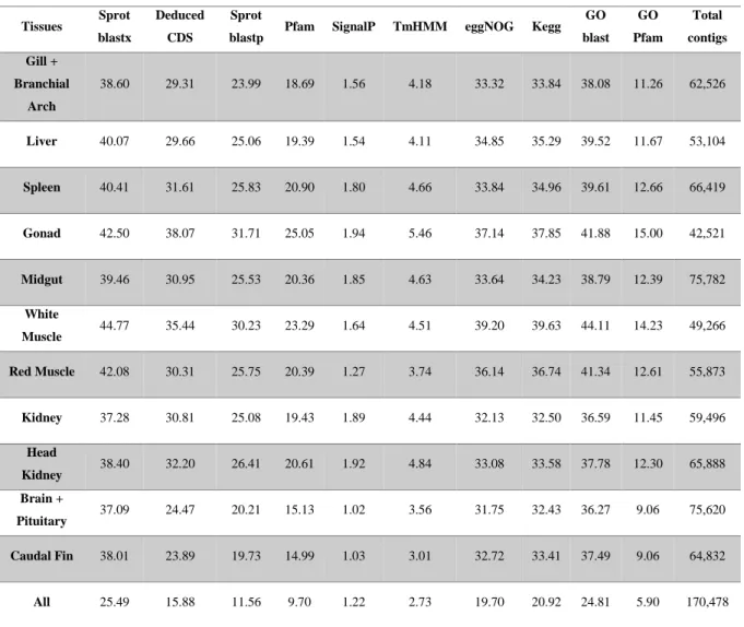
Table 3.5: Percentages of annotated transcripts per tissue.

Tissues Sprot blastx

Deduced CDS

Sprot

blastp Pfam SignalP TmHMM eggNOG Kegg GO blast GO Pfam Total contigs Gill + Branchial Arch 38.60 29.31 23.99 18.69 1.56 4.18 33.32 33.84 38.08 11.26 62,526 Liver 40.07 29.66 25.06 19.39 1.54 4.11 34.85 35.29 39.52 11.67 53,104 Spleen 40.41 31.61 25.83 20.90 1.80 4.66 33.84 34.96 39.61 12.66 66,419 Gonad 42.50 38.07 31.71 25.05 1.94 5.46 37.14 37.85 41.88 15.00 42,521 Midgut 39.46 30.95 25.53 20.36 1.85 4.63 33.64 34.23 38.79 12.39 75,782 White Muscle 44.77 35.44 30.23 23.29 1.64 4.51 39.20 39.63 44.11 14.23 49,266 Red Muscle 42.08 30.31 25.75 20.39 1.27 3.74 36.14 36.74 41.34 12.61 55,873 Kidney 37.28 30.81 25.08 19.43 1.89 4.44 32.13 32.50 36.59 11.45 59,496 Head Kidney 38.40 32.20 26.41 20.61 1.92 4.84 33.08 33.58 37.78 12.30 65,888 Brain + Pituitary 37.09 24.47 20.21 15.13 1.02 3.56 31.75 32.43 36.27 9.06 75,620 Caudal Fin 38.01 23.89 19.73 14.99 1.03 3.01 32.72 33.41 37.49 9.06 64,832 All 25.49 15.88 11.56 9.70 1.22 2.73 19.70 20.92 24.81 5.90 170,478

Table 3.6: Percentages of annotated transcripts before and after Transrate filtration on the

caudal fin tissue.

Caudal Fin Sprot blastx

Deduced CDS

Sprot

blastp Pfam SignalP TmHMM eggNOG Kegg GO blast GO Pfam Total contigs Before Transrate 37.29 24.17 19.34 15.16 1.37 3.30 31.48 32.31 36.67 9.24 64,832 After Transrate 38.01 23.89 19.73 14.99 1.03 3.01 32.72 33.41 37.49 9.06 98,276

Table 3.7: Percentages of annotated transcripts contigs before and after Transrate filtration on

the assembly containing reads from all the tissues.

All Tissues Sprot blastx

Deduced CDS

Sprot

blastp Pfam SignalP TmHMM eggNOG Kegg GO blast GO Pfam Total contigs Before Transrate 33.89 26.95 21.11 18.46 2.42 5.14 27.37 28.32 32.98 11.49 385,373 After Transrate 25.49 15.88 11.56 9.70 1.22 2.73 19.70 20.92 24.81 5.90 170,478