Intelligent support system for CVA diagnosis by cerebral computerized tomography

(1)

ELMIRA HAJIMANI

INTELLIGENT SUPPORT SYSTEM FOR CVA

DIAGNOSIS BY CEREBRAL COMPUTERIZED

TOMOGRAPHY

UNIVERSIDADE DO ALGARVE

Faculdade de Cîencias e Tecnologia

2016

(2)

(3)

ELMIRA HAJIMANI

INTELLIGENT SUPPORT SYSTEM FOR CVA

DIAGNOSIS BY CEREBRAL COMPUTERIZED

TOMOGRAPHY

Doutoramento em Engenheira Informática

(Especialidade em Inteligência Artificial)

Trabalho efeuado sob a orientação de:

António Eduardo de Barros Ruano e Maria da Graça Ruano

UNIVERSIDADE DO ALGARVE

Faculdade de Cîencias e Tecnologia

2016

(4)

(5)

INTELLIGENT SUPPORT SYSTEM FOR CVA DIAGNOSIS BY CEREBRAL COMPUTERIZED TOMOGRAPHY

Declaração de autoria de trabalho

Declaro ser a autora deste trabalho, que é original e inédito. Autores e trabalhos consultados estão devidamente citados no texto e constam da listagem de referências incluída.

_________________________________________________ Elmira Hajimani

Copyright: Elmira Hajimani

A Universidade do Algarve reserva para si o direito, em conformidade com o disposto no Código do Direito de Autor e dos Direitos Conexos, de arquivar, reproduzir e publicar a obra, independentemente do meio utilizado, bem como de a divulgar através de repositórios científicos e de admitir a sua cópia e distribuição para fins meramente educacionais ou de investigação e não comerciais, conquanto seja dado o devido crédito ao autor e editor respetivos.

(6)

(7)

To my love, Hamid

To my parents, Zari and Majid

To my sister, Armita

(8)

(9)

Acknowledgement

First and foremost, I would like to express my deepest thanks and appreciation to my supervisors, Prof. António Ruano and Prof. Graça Ruano, for having provided me with their expertise, valuable advice, direction and suggestions during the past four years. Without their inspiration, support and encouragement, this dissertation would have been impossible.

I would particularly like to acknowledge the Erasmus Mundus EMIIY scholarship program for its financial support of this thesis. I also would like to express my gratitude to Prof. Hamid Shahbazkia as the coordinator of EMIIY scholarship program for all his kind supports.

I wish to acknowledge Dr. Luis Cerqueira, from Centro Hospitalar de Lisboa Central, Portugal, for marking the CT exams, Mr. Sergio Silva, in CSI Laboratory, for his precious help in solving implementation issues and Dr. Carina Ruano for her helpful suggestions while we were designing our web based tool for marking CVA lesions in CT images. I am also grateful to the staff of mobility office at the University of Algarve for all their supports.

My sincere appreciation goes to my dear friend, Dr. Eslam Nazemi, for his continuous encouragement and support during the past 10 years of my academic life. Dr. Nazemi brought me to the world of academic research and supervised my B.Sc. and M.Sc. dissertations.

I would like to express my deepest gratitude to my beloved husband and my great colleague, soon to be Dr. Hamid Reza Khosravani, for his endless love, unconditional support, for all the joyful moments we built together and for long hours of scientific discussions.

Last but not least, my special thanks goes to my beloved parents and my sister who taught me how to think and how to love.

(10)

(11)

i

Abstract

The Cerebral Vascular Accident (CVA) is one of the major causes of death in USA and developed countries, immediately following cardiac diseases and tumors. The increasing number of CVA’s and the requirement of short time diagnosis to minimize morbidity and mortality encourages the development of computer aided diagnosis systems. Early stages of CVA are often undetected by human eye observation of Computer Tomographic (CT) images, thus incorporation of intelligent based techniques on such systems is expected to highly improve their performance.

This thesis presents a Radial Basis Functions Neural Network (RBFNN) based diagnosis system for automatic identification of CVA through analysis of CT images. The research hereby reported included construction of a database composed of annotated CT images, supported by a web-based tool for Neuroradiologist registration of his/her normal or abnormal interpretation of each CT image; in case of an abnormal identification the medical doctor was indicted by the software application to designate the lesion type and to identify the abnormal region on each CT’s slice image.

Once provided the annotated database each CT image processing considered a pre-processing stage for artefact removal and tilted images’ realignment followed by a feature extraction stage.

A large number of features was considered, comprising first and second order pixel intensity statistics as well as symmetry/asymmetry information with respect to the ideal mid-sagittal line of each image.

The policy conducted during the intelligent-driven image processing system development included the design of a neural network classifier. The architecture was determined by a Multi Objective Genetic Algorithm (MOGA) where the classifier structure, parameters and image features (input features) were chosen based on the use of different (often conflicting) objectives, ensuring maximization of the classification precision and a good generalization of its performance for unseen data

Several scenarios of choosing proper MOGA’s data sets were conducted. The best result was obtained from the scenario where all boundary data points of an enlarged dataset were included in the MOGA training set.

(12)

ii

Confronted with the NeuroRadiologist annotations, specificity values of 98.01% and sensitivity values of 98.22% were obtained by the computer aided system, at pixel level. These values were achieved when an ensemble of non-dominated models generated by MOGA in the best scenario, was applied to a set of 150 CT slices (1,867,602 pixels).

Present results show that the MOGA designed RBFNN classifier achieved better classification results than Support Vector Machines (SVM), despite the huge difference in complexity of the two classifiers. The proposed approach compares also favorably with other similar published solutions, both at lesion level specificity and at the degree of coincidence of marked lesions.

Keywords: Neural Networks; Symmetry features; Multi-Objective Genetic Algorithm; Intelligent

(13)

iii

Resumo

Os Acidentes Vasculares Cerebrais (AVC) são uma das maiores causas de morte nos EUA e em países desenvolvidos, imediatamente a seguir a condições cardícas e a tumores. O aumento do número de AVCs e o requisito de um diagnóstico rápido, necessário para minimizar a morbilidade e a mortalidade, encoraja o desenvolvimento de sistemas de ajuda ao diagnóstico. Os CVAs, num estado inicial não conseguem muitas vezes serem detetados pelo observação humana de imagens de Tomografia Computorizada (TC); a incorporação de técnicas baseadas em inteligência computacional poderá contribuir para melhorar a performance desses sistemas.

Esta tese apresenta um sistema de diagnóstico baseado em Redes Neuronais de Função de Base Radial (RNFBR) para a identificação automática de AVCs através da análise de imagens de TC. A investigação reportada nesta Tese incluiu a construção de uma base de dados de imagens de TC anotadas, suportadas por uma ferramenta baseada na Web que permite que os Neuroradiologistas registem as lesões por si identificadas, bem como o tipo de lesão e a região do cérebro onde a mesma se localiza.

Após criação da base de dados anotada, as imagens de TC são submetidas a um passo de pré-processamento, incluindo remoção de artefactos e realinhamento das imagens inclinadas,de modo a poder-se posteriormente proceder à extração de características.

Um grande número de características de entrada são considerados nesta abordagem, compreendendo estatísticas de primeira e segunda ordem dos pixéis da imagem, , bem como informações de simetria ou assimetria em relação à linha média sagital ideal.

Para a conceção de um classificador da rede neuronal, é utilizada uma abordagem baseada num Algoritmo Genético Multi-Objectivo (MOGA) para determinar a arquitetura do classificador, os seus parâmetros, bem como as características de entrada utilizadas, utilizando para tal diferentes objetivos, muitas vezes conflituosos entre si, aumentando a precisão de classificação sem no entanto comprometer a sua generalização para dados não consierados no projeto da rede.

Foram realizados vários cenários em MOGA. O melhor resultado foi obtido do cenário no qual no conjunto de treino de MOGA foram incorporados os vértices do fecho convexo de um conjunto alargado de pixéis.

(14)

iv

Confrontando com as anotações do Neuroradiologista, foi sistema obteve valores de especificidade de 98,01% e sensibilidade de 98,22%, ao nível do pixel. Estes resultados foram obtidos por um conjunto de modelos não-dominados gerados pelo MOGA no melhor cenário, num conjunto de 150 imagens TC (1,867,602 pixels).

Esta abordagem compara-se muito favoravelmente com outras soluções semelhantes publicadas, tanto em especificidade ao nível da lesão, como no grau de coincidência de lesões marcadas. Comparando os resultados da classificação neuronal com Máquinas de Vetor de Suporte (SVM), é evidente que, apesar da enorme complexidade do modelo SVM, a precisão do modelo neuronal é superior à do modelo SVM.

Palavras-chave: Redes Neuronais; Algoritmo Genético Multi-Objectivo; Acidentes Vasculares

(15)

v

List of Tables

Table 3.1 Properties of brain imaging modalities ... 46

Table 3.2 Properties of four medical image formats [60] ... 47

Table 3.3 Hounsfield Units of brain tissues in CT images [62] ... 49

Table 4.1 Different types of brain lesions are marked by different colours in each CT image ... 83

Table 4.2 Components of neighbourhood lookup arrays in K3M algorithm ... 87

Table 5.1 Our primary feature space ... 98

Table 5.2 DS(1) specification ... 103

Table 5.3 Top 5% models of scenario 1 in terms of number of FN in BIG_DS ... 103

Table 5.4 Top 5% models of scenario 1 in terms of number of FP in BIG_DS ... 104

Table 5.6 Models of scenario 2 whose number of FPs and FNs is less than or equal to 6% in 𝑩𝑰𝑮_𝑫𝑺 ... 106

Table 5.8 Models of scenario 3 whose number of FPs and FNs is less than 7% in 𝑩𝑰𝑮_𝑫𝑺 ... 109

Table 5.9 𝑫𝑺(𝟒𝒂) specification ... 110

Table 5.10 Models of scenario 4 whose number of FPs and FNs is less than 7% in 𝑩𝑰𝑮_𝑫𝑺 .... 111

Table 5.11 𝑫𝑺(𝟒𝒃) specification ... 112

Table 5.12 Models of scenario 4-second round whose number of FPs and FNs is less than 8% in 𝑩𝑰𝑮_𝑫𝑺 ... 113

Table 5.13 𝑫𝑺(𝟓𝒂) specification ... 114

Table 5.14 Models of scenario 5-first round whose number of FPs and FNs is less than 8% in 𝑩𝑰𝑮_𝑫𝑺 ... 115

(20)

x

Table 5.16 Models of scenario 5-second round whose number of FPs and FNs is less than 11% in

𝑩𝑰𝑮_𝑫𝑺 ... 117

Table 5.17 𝑫𝑺(𝟔) specification ... 118

Table 5.18 Top 1% models of scenario 6 in terms of FN rate in BIG_DS ... 119

Table 5.19 Top 1% models of scenario 6 in terms of FP rate in BIG_DS ... 119

Table 5.20 𝑫𝑺(𝟔𝒂) specification ... 120

Table 5.21 Models of scenario 6-first round of active learning whose number of FPs and FNs is less than 10% in 𝑩𝑰𝑮_𝑫𝑺 ... 121

Table 5.22 𝑫𝑺(𝟔𝒃) specification ... 122

Table 5.23 Models of scenario 6-second round of active learning whose FP and FN rates are less than 6% in 𝑩𝑰𝑮_𝑫𝑺 ... 122

Table 5.24 𝑫𝑺(𝟔𝒄) specification ... 124

Table 5.25 Models of scenario 6-third round of active learning whose of FP rate is less than 5% in 𝑩𝑰𝑮_𝑫𝑺 ... 125

Table 5.26 𝑫𝑺(𝟔𝒅) specification ... 125

Table 5.27 Top 1% models of scenario 6 - 4th_{round of active learning in terms of FN rate in} 𝑩𝑰𝑮_𝑫𝑺 ... 126

Table 5.28 Top 1% models of scenario 6 -4th_{round of active learning in terms of FP rate in} 𝑩𝑰𝑮_𝑫𝑺 ... 127

Table 5.29 Models of scenario 6-4th_{round of active learning with restricted MOGA objectives} whose of FP and FN rates over 𝑩𝑰𝑮_𝑫𝑺 are less than 5.5% ... 128

Table 5.30 𝑫𝑺(𝟕) specification ... 129

Table 5.31Min, Avg. and Max false positive and false negative rates as well as model complexity of 406 non-dominated models of scenario 7. ... 129

Table 5.32 Models of scenario 7 whose of FP and FN rates over 𝑩𝑰𝑮_𝑫𝑺 are less than 3% ... 130

(21)

xi

Table 5.34. Min, Avg. and Max false positive and false negative rates as well as model

complexity of 69 models in preferable set of 𝒔𝒄𝒆𝒏𝒂𝒓𝒊𝒐 𝟕𝒃. ... 131 Table 5.35 Models of 𝒔𝒄𝒆𝒏𝒂𝒓𝒊𝒐 𝟕𝒃 whose FP and FN rates over 𝑩𝑰𝑮_𝑫𝑺 are less than 2.6% 131 Table 5.36 Comparing best models of all scenarios ... 133 Table 5.37 The result of applying ensemble of preferable models of 𝒔𝒄𝒆𝒏𝒂𝒓𝒊𝒐 𝟕𝒃 on 𝑴𝑶𝑮𝑨_𝑫𝑺 and 𝑩𝑰𝑮_𝑫𝑺 ... 134 Table 5.38 FP and FN rates using SVM... 135 Table 5.39. Colour code used for marking pixels based on the percentage of preferable models with a positive output ... 137

(22)

(23)

xiii

List of Figures

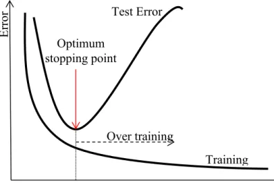
Fig. 2.1 A taxonomy of neural network architectures [11] ... 6 Fig. 2.2 Multi-layer Perceptron with two hidden layers. ... 8 Fig. 2.3 Radial Basis Functions Neural Network with one hidden layer. ... 9 Fig. 2.4 A taxonomy of learning algorithms from three different points of view [11] ... 11 Fig. 2.5 The dependency of gradient descent on the initial parameters’ value ... 12 Fig. 2.6 Example of one step of Newton’s method ... 15 Fig. 2.7 An example of overfitted models and models with good generalization ... 22 Fig. 2.8 Early stopping approach stops the training process at the optimum point to have a

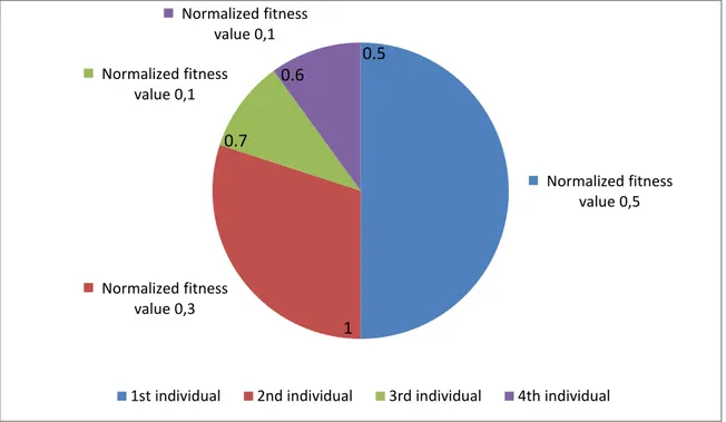
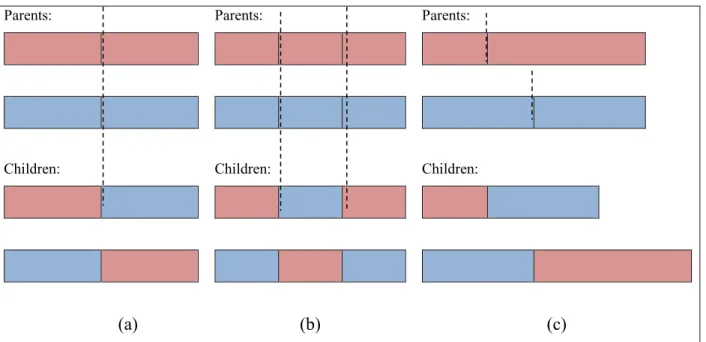
generalized model. ... 22 Fig. 2.9 An example of a separable problem in a 2 dimensional space. The support vectors, marked with red circles, define the margin of largest separation between the two classes [26]. ... 23 Fig. 2.10 Roulette wheel of 4 individuals. The accumulated normalized value of each individual is written inside the corresponding portion. ... 26 Fig. 2.11 Three different methods of crossover; (a) One-point crossover; (b) Two-point

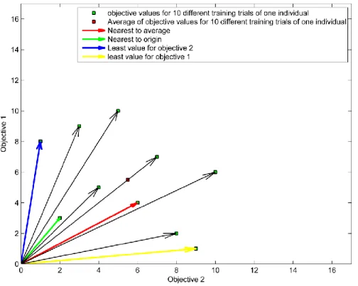
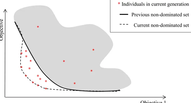
crossover; (c) Cut and splice crossover. ... 27 Fig. 2.12 Pareto ranking [34, 35] ... 29 Fig. 2.13 Pareto ranking in the case that both objectives have equal priorities. Both objectives should meet the defined goals [32, 36]. ... 30 Fig. 2.14 Pareto ranking in the case that objective 2 has higher priority than objective 1. Both objectives should meet the defined goals [32, 36]. ... 30 Fig. 2.15 The topology of the chromosome ... 32 Fig. 2.16 Four different strategies for identifying the best training trial within α times training. . 33 Fig. 2.17 The update of non-dominated set on arrival of new points ... 34 Fig. 2.18 Active learning vs. Passive learning [38] ... 35 Fig. 2.19 (a) represents a convex set; (b) represents a non-convex set. ... 36

(24)

xiv

Fig. 2.20 Vertices and facets of convex hull in (a) two dimensional space and (b) three

dimensional space. ... 37 Fig. 3.1 Brain CT slice with (a) Ischemic stroke [51]. (b) Haemorrhagic stroke [52]. ... 44 Fig. 3.2 Raw CT slices from one patient’s head CT ... 52 Fig. 3.3 Artifact removal process proposed in [67]. (a) The original image. (b) The largest

connected component is selected as the skull after applying the threshold. (c) Small holes are filled. (d) The centre of mass of the skull is found (blue point). (e) The cranial part is filtered based on the centre of mass location. ... 53 Fig. 3.4 Applying Algorithm 3.1 on raw CT images of Fig. 3.2 ... 54 Fig. 3.5 Applying Algorithm 3.2 on raw CT images of Fig. 3.2. The yellow line is the ideal midsagittal line after rotating CT slices. The red point is the mass centre of the skull. ... 57 Fig. 3.6 (a) and (b) are two different images with same first order statistics features [97] ... 63 Fig 3.7 (a) Magnified part of brain image (yellow square); (b) represents corresponding intensity values in range [0 255]; (c) intensity values are scaled into range [1 8]. ... 66 Fig. 3.8 Visualizing different values of 𝜽 for constructing GLCM ... 67 Fig. 3.9 GLCM calculation in different directions for image matrix shown in Fig. 3.7-c ... 68 Fig. 3.10: (a) Original brain CT image; (b) After skull removal and realignment, ideal midline is drawn in yellow color. The green point shows the mass centre (centroid) of skull. A window of size 31x31 is considered around pixel located at (365,279) and shown in red color; its

contralateral part with respect to the midline is shown in blue color. ... 74 Fig. 4.1 General diagram of the Web-based tool for registering and identification of pathological areas in CT images ... 76 Fig. 4.2 Diagram of possible activities of the user Administrator ... 77 Fig. 4.3 Administrator interface for uploading new CT images. ... 78 Fig. 4.4 (a) left side shows the structure of zip file containing Neuradiologists’ opinions; right side shows the content of text file which determines the coordinate and type of lesion pixels including the ones that are already marked in (b). ... 79

(25)

xv

Fig. 4.5 (a) Administrator interface where the last link is for downloading Neuroradiologists’ opinions; (b) Administrator interface for creating new users. ... 80 Fig. 4.6 User interface for displaying list of CT exams to Neuroradiologist ... 81 Fig. 4.7 User Interface for registering pathological areas ... 82 Fig. 4.8(a), (d) Green pixels shows the drawn contours; the first one is open and the second one is closed. (b), (e) the transparent layers of the processed contours. (c), (f) the transparent layers are super imposed on the original image. ... 83 Fig. 4.9 Diagram of possible activities of other users, namely Neuroradiologists ... 84 Fig. 4.10 Global diagram of the database of the web-based tool ... 86 Fig. 4.11 K3M algorithm simplified flowchart ... 88 Fig. 4.12 Flowchart of phase 0 (marking border) of K3M algorithm. ... 89 Fig. 4.13 Flowchart of Phase 𝒊 = 𝟏, 𝟐, 𝟑, 𝟒, 𝟓, 𝟔 deleting pixels. ... 90 Fig. 4.14 User hand Drawn contour on CT image in green color (a); Applying K3M algorithm to make the drawn contour one pixel width (b). Blue pixels will not be considered as part of the contour anymore. ... 91 Fig. 5.1 𝑬𝒙𝒂𝒎𝒔(𝒊) structure containing the information about one CT exam. ... 97 Fig. 5.2 The result of applying the ensemble of preferable models of 𝒔𝒄𝒆𝒏𝒂𝒓𝒊𝒐 𝟕𝒃 on 11 CT images. The left column shows the original images. In the middle column the lesions marked by the Neuroradialogist are shown. In the right column the pixels are marked by the classifier. .... 141 Fig. 5.3 Normalized frequency of each feature in preferable models of 𝒔𝒄𝒆𝒏𝒂𝒓𝒊𝒐 𝟕𝒃. ... 142 Fig. 5.4 𝑫𝑨𝑫𝑯𝒔 values for 51 features in our feature space. ... 143 Fig. A.1 Definition of the boxplot features [126] ... A-5 Fig. A.2: (a) bi-histogram of Feature 1; (b) box plot of Feature 1. ... A-7 Fig. A.3 Mean values of each feature for normal and abnormal sub-groups of pixels ... A-8 Fig. A.4: (a) bi-histogram of Feature 2; (b) box plot of Feature 2. ... A-9 Fig. A.5: (a) bi-histogram of Feature 3; (b) box plot of Feature 3. ... A-11 Fig. A.6: (a) bi-histogram of Feature 4; (b) box plot of Feature 4. ... A-13

(26)

xvi

Fig. A.7: (a) bi-histogram of Feature 5; (b) box plot of Feature 5. ... A-14 Fig. A.8: (a) bi-histogram of Feature 6; (b) box plot of Feature 6. ... A-16 Fig. A.9: (a) bi-histogram of Feature 7; (b) box plot of Feature 7. ... A-17 Fig. A.10: (a) bi-histogram of features 8; (b) box plot of features 8. ... A-19 Fig. A.11: (a) bi-histogram of features 9; (b) box plot of features 9. ... A-20 Fig. A.12: (a) bi-histogram of features 10; (b) box plot of features 10. ... A-22 Fig. A.13: (a) bi-histogram of features 11; (b) box plot of features 11. ... A-23 Fig. A.14: (a) bi-histogram of features 12; (b) box plot of features 12. ... A-25 Fig. A.15: (a) bi-histogram of features 13; (b) box plot of features 13. ... A-27 Fig. A.16: (a) bi-histogram of features 14; (b) box plot of features 14. ... A-28 Fig. A.17: (a) bi-histogram of features 15; (b) box plot of features 15. ... A-30 Fig. A.18: (a) bi-histogram of features 16; (b) box plot of features 16. ... A-31 Fig. A.19: (a) bi-histogram of features 17; (b) box plot of features 17. ... A-33 Fig. A.20: (a) bi-histogram of features 18; (b) box plot of features 18. ... A-34 Fig. A.21: (a) bi-histogram of features 19; (b) box plot of features 19. ... A-36 Fig. A.22: (a) bi-histogram of features 20; (b) box plot of features 20. ... A-37 Fig. A.23: (a) bi-histogram of features 21; (b) box plot of features 21. ... A-39 Fig. A.24: (a) bi-histogram of features 22; (b) box plot of features 22. ... A-41 Fig. A.25 Visualizing inverse relationship between energy and dissimilarity features ... A-41 Fig. A.26 Visualizing inverse relationship between energy and entropy features ... A-43 Fig. A.27: (a) bi-histogram of features 23; (b) box plot of features 23. ... A-43 Fig. A.28: (a) bi-histogram of features 24; (b) box plot of features 24. ... A-45 Fig. A.29: (a) bi-histogram of features 25; (b) box plot of features 25. ... A-46 Fig. A.30: (a) bi-histogram of features 26; (b) box plot of features 26. ... A-47 Fig. A.31: (a) bi-histogram of features 27; (b) box plot of features 27. ... A-49

(27)

xvii

Fig. A.32: (a) bi-histogram of features 28; (b) box plot of features 28. ... A-50 Fig. A.33: (a) bi-histogram of features 29; (b) box plot of features 29. ... A-51 Fig. A.34: (a) bi-histogram of features 30; (b) box plot of features 30. ... A-53 Fig. A.35: (a) bi-histogram of features 31; (b) box plot of features 31. ... A-54 Fig. A.36: (a) bi-histogram of features 32; (b) box plot of features 32. ... A-55 Fig. A.37: (a) bi-histogram of features 33; (b) box plot of features 33. ... A-57 Fig. A.38: (a) bi-histogram of features 34; (b) box plot of features 34. ... A-58 Fig. A.39: (a) bi-histogram of features 35; (b) box plot of features 35. ... A-59 Fig. A.40: (a) bi-histogram of features 36; (b) box plot of features 36. ... A-60 Fig. A.41: (a) bi-histogram of features 37; (b) box plot of features 37. ... A-62 Fig. A.42: bi-histograms and box plots of features 38 (𝑭𝟏), 39 (𝑭𝟐), 40 (𝑭𝟑) and 41 (𝑭𝟒). ... A-64 Fig. A.43: bi-histograms and box plots of PCC feature with different window sizes 𝟑𝟏 × 𝟑𝟏 (Feature 42), 𝟐𝟏 × 𝟐𝟏 (Feature 46) and 𝟏𝟏 × 𝟏𝟏 (Feature 49). ... A-66 Fig. A.44: (a) bi-histogram of features 43; (b) box plot of features 43. ... A-67 Fig. A.45: bi-histograms and box plots of 𝑳𝟏 feature with different window sizes 𝟑𝟏 × 𝟑𝟏 (Feature 44), 𝟐𝟏 × 𝟐𝟏 (Feature 47) and 𝟏𝟏 × 𝟏𝟏 (Feature 50). ... A-69 Fig. A.46: bi-histograms and box plots of 𝐋𝟐𝟐 feature with different window sizes 𝟑𝟏 × 𝟑𝟏 (Feature 45), 𝟐𝟏 × 𝟐𝟏 (Feature 48) and 𝟏𝟏 × 𝟏𝟏 (Feature 51). ... A-71

(28)

(29)

xix

List of Algorithms

Algorithm 2.1 Using k-means clustering to find RBFNN centers [21] ... 20 Algorithm 3.1 Artifact removal algorithm in brain CT images [67] ... 50 Algorithm 3.2 Ideal midline detection of the brain CT images [67, 73] ... 56 Algorithm 4.1 Detecting the discontinuity of the drawn contour around lesion ... 91 Algorithm 5.1 Obtaining the coordinate of normal pixels ... 96

(30)

(31)

xxi

List of Acronyms

ABR Area of Bleeding Region

ADH Amplitude Distribution Histograms AER Area of Edema Region

AMM Adaptive Mixtures Method ANNs Artificial Neural Networks

BP Back Propagation

CAD Computer Aided Diagnosis

CAROI Circular Adaptive Region of Interest CLBP Completed Local Binary Pattern

CLBP_C Completed Local Binary Pattern - Center CLBP_M Completed Local Binary Pattern - Magnitude CLBP_S Completed Local Binary Pattern -Sign CRLBP Completed Robust Local Binary Pattern CSF Cerebrospinal Fluid

CT Computerized Tomography

CVA Cerebral Vascular Accident DFP Davidson–Fletcher–Powell DOT Diffuse Optical Tomography EDA Exploratory Data Analysis EM Expectation Maximization

(32)

xxii ESMF Edge-based Selective Median Filter FCM Fuzzy C-Means

fMRI functional Magnetic Resonance Imaging

FN False Negative

FP False Positive

GA Genetic Algorithm

GLCM Gray Level Co-occurrence Matrix

GM Gray Matter

HU Hounsfield Units

IDM Inverse Difference Moment k-NN k-Nearest Neighbors

LBP Local Binary Pattern

LM Levenberg-Marquardt

LTP Local Ternary Pattern

LRHGE Long Run High Gray Level Emphasis LRLGE Long Run Low Gray Level Emphasis MLP Multi-Layer Perceptron

MOGA Multi Objective Genetic Algorithm

MR Magnetic Resonance

MRI Magnetic Resonance Imaging

(33)

xxiii PCC Pearson Correlation Coefficient PET Positron Emission Tomography PSM Power Spectrum Method

RBFNN Radial Basis Functions Neural Network SMOTE Synthetic Minority Over-sampling Technique

SMOTE-N Synthetic Minority Over-sampling Technique Nominal

SMOTE-NC Synthetic Minority Over-sampling Technique Nominal Continuous SR1 Symmetric Rank one

SRHGE Short Run High Gray Level Emphasis SRLGE Short Run Low Gray Level Emphasis SUS Stochastic Universal Sampling SVM Support Vector Machine WM White Matter

(34)

(35)

1

1. Introduction

The Cerebral Vascular Accident is the third cause of death in USA, immediately following cardiac diseases and tumors. In the USA, from the 700.000 CVA cases, 600.000 are ischemic and 100.000 hemorrhagic. 175.000 CVAs are fatal, and the rest reduces patients’ morbidity, involving additional expenses for the National Health Systems [1]. In Portugal the CVA is the first cause of death, and several studies point out a prognosis of more than 80 CVA occurrences per day for the next 10 years.

Computerised Tomography (CT) is one of the imaging equipments for diagnosis which benefited more from technological improvements. Because of that, and due to the quality of the diagnosis produced, it is one of the most used equipments in clinical applications. For CVA diagnosis, CT is the elected imaging equipment, as the majority of hospitals have CTs, but no Magnetic Resonance (MR) equipment. In those where MR is available, it is typically used only at 1/3 of the day, due to the need for specialized personnel, which is lacking. However, within the first few hours after symptom onset, the interpretation of CT images can be difficult due to the inconspicuousness of the lesions. Quick diagnosis becomes even more difficult when the CT technician is not familiar with image post-processing protocols.

These facts constitute the motivation to create an intelligent application capable of assisting the CT technician on triggering a pathologic occurrence and enabling a better performance of CVA detection.

1.1 Objectives

This PhD aimed to construct a prototype of an automatic support system for CVA diagnosis in CTs, by:

1. Providing a platform to enlarge the existing “storage” of diagnosed CT scans, and implementing a proper database.

2. To account for the variability found in CT scans, carefully reviewing the features used for classification.

(36)

2

3. Using the available multi-objective evolutionary methodology for designing neural classifiers to select the most relevant features [2]. The referred system allows, besides designing the classifier topology and determining its parameters, to perform feature selection, according to different objectives and priorities. In contrast with the existing approaches found in the literature, where features are taken solely from one specific category (i.e., first order or second order statistics), our system will pick up the most important features from the union of these sets as well as incorporating some symmetry features.

4. Performing medical validation of the prototype system.

1.2 Major contributions

A web-based tool was developed [3] in order to be able to register the opinion of Neuroradiologists for each CT image. Using this tool, a database of CT images was created for Neuroradiologists to remotely analyze and mark the images either as normal or abnormal. For the abnormal ones, the doctor is able to identify the lesion type and the abnormal region on each CT’s slice image. A thorough review has been done on the features used by other works (i.e., Please refer to section 3.7). Table 5.1 provide a list of features that are used in this work. These features can be grouped into three main categories:

a) First order statistics which estimate properties of individual pixel values, ignoring the spatial interaction between image pixels.

b) Second order statistics which estimate properties of two pixel values occurring at specific locations relative to each other.

c) Features related with differences in symmetry across the ideal midsagittal plane.

To our knowledge, none of existing classifiers learn about the asymmetry caused by lesions in intracranial area. In this work, a group of symmetry features that were proposed in [4], are going to be used along with other statistical features to add the ability of detecting asymmetries (with respect to ideal mid-sagittal line ) to the designed classifier.

Several experiments were conducted in MOGA and the corresponding obtained models were evaluated using a set of 1,867,602 pixels. In some experiments, active learning approach is applied

(37)

3

to design the subsequent experiment. To construct the dataset of the conducted experiments, Approxhull [5, 6] is used to incorporate convex points in the training set. This will help MOGA to see the whole range of the data where the classifier is going to be used.

The best result is obtained from an ensemble of preferable models of the experiment whose training set contained all convex points of the 1,867,602 pixels together with some random normal and abnormal pixels. Values of specificity of 98.01% (i.e., 1.99 % False Positive) and sensitivity of 98.22% (i.e., 1.78% False Negative) were obtained at pixel level, in a set of 150 CT slices (1,867,602 pixels).

Comparing the classification results with SVM, shows that, despite the huge complexity of SVM model, the accuracy of the ensemble of preferable models is superior to that of SVM model. The present approach compares favorably with other similar (although with not the same specifications) published approaches [7, 8], achieving, on the one hand, improved sensitivity at lesion level, and, on the other hand, superior average difference and degree of coincidence between lesions marked by the doctor and marked by the automatic system.

As a result of the research work developed under this PhD thesis the following publications were produced:

• E. Hajimani, M. G. Ruano, and A. E. Ruano, "An Intelligent Support System for Automatic Diagnosis of Cerebral Vascular Accidents from Brain CT Images," submitted to Computer Methods and Programs in Biomedicine (May 2016)

• M. G. Ruano, E. Hajimani, and A. E. Ruano, "A Radial Basis Function Classifier for the Automatic Diagnosis of Cerebral Vascular Accidents," presented at the Global Medical Engineering Physics Exchanges/Pan American Health Care Exchanges (GMEPE / PAHCE), Madrid, Spain, 2016.

• E. Hajimani, M. G. Ruano, and A. E. Ruano, "MOGA design for neural networks based system for automatic diagnosis of Cerebral Vascular Accidents," in 9th IEEE International Symposium on Intelligent Signal Processing (WISP), 2015, pp. 1-6.

(38)

4

• E. Hajimani, A. Ruano, and G. Ruano, "The Effect of Symmetry Features on Cerebral Vascular Accident Detection Accuracy," presented at the RecPad 2015, the 21th edition of the Portuguese Conference on Pattern Recognition, Faro, Portugal, 2015.

• E. Hajimani, C. A. Ruano, M. G. Ruano, and A. E. Ruano, "A software tool for intelligent CVA diagnosis by cerebral computerized tomography," in 8th IEEE International Symposium on Intelligent Signal Processing (WISP), 2013, pp. 103-108.

1.3 Thesis structure

This thesis is organized in 6 chapters. Chapter 2 gives a brief overview on the theoretical background that is needed to develop this work. This includes a review on artificial neural networks and learning algorithms, Support Vector Machines, Multi-Objective Genetic Algorithm, active learning, Approxhull and existing solutions for dealing with the challenge of classifying imbalanced datasets.

Chapter 3 gives the necessary background information about Cerebral Vascular Accident, medical imaging techniques and the state of the art for automatic segmentation of lesions from brain tissues in medical images. A review on textural feature extraction methods is also presented in this chapter. To train, test and validate the neural network models for classifying pathologic areas within brain CT images, it is necessary to acquire the opinion of Neuroradiologists, and use it as the gold standard. Chapter 4 presents our developed web-based tool to collect this information in an accurate and convenient way. Having used our developed web-based tool to obtain the opinion of the Neuroradiologist about existing CT images, we are now able to construct our dataset.

Chapter 5 starts with describing how we produced our datasets from the CT images previously marked by Neuroradiologist. To obtain the best possible RBFNN classifier, several scenarios were conducted in MOGA which are explained in chapter 5. This chapter also shows the results obtained, including visualization of the estimated abnormal regions in CT images, and compares the proposed approach with support vector machines and two other Computer Aided Diagnosis (CAD) systems. Finally, a discussion on the discrimination power of the most frequent features in preferable models of the best scenario is performed.

(39)

5

2. Intelligent systems background

This chapter aims to review the basic concepts of intelligent data driven modeling techniques that are used for developing the presented intelligent support system for automatic diagnosis of Cerebral Vascular Accident from brain Computed Tomography images. Intelligent data driven modeling can be thought as the use of a collection of approaches, mainly artificial neural networks, fuzzy rule-based systems and evolutionary algorithms to build models, calibrate them and optimize their structures. For building models, data driven approaches use available data to develop relationships between the input and output variables involved in the actual process. The presented work uses a combination of neural networks and genetic algorithms methods to build the proposed system. The chapter is organized as follows: Section 2.1 gives a brief overview on Artificial Neural Networks. In this section, after providing a taxonomy of existing neural network topologies, a more detailed discussion is done on Multi-Layered Perceptron and Radial Basis Functions Neural Networks. An overview on different learning algorithms with the focus on supervised algorithms is done afterwards. Section 2.1 continues with the presentation of three learning strategies for Radial Basis Functions Neural Networks. Termination criteria for the training process are discussed in the last part of section 2.1. A brief description of Support Vector Machines is presented in section 2.2 since we have compared our work with this method in later chapters. Multi-Objective Genetic Algorithm, as a framework to determine the architecture of the classifier, its corresponding parameters and input features according to the multiple objectives imposed and their corresponding restrictions and priorities, is discussed in section 2.3. Section 2.4 discusses active learning as a way of choosing the most informative data samples from a pool of data. Approxhull, as a data selection approach for selecting the most suitable data to be incorporated in the training set, is presented in section 2.5. Section 2.6 overviews potential solutions for dealing with the challenge of classifying imbalanced datasets.

2.1 Artificial Neural Networks

Artificial Neural Networks were initially developed as an attempt to mimic the behavior of human brain. As we know, human brain can be divided into regions, each of which specialized in different functions. But the interesting point is that one region of the brain has the capacity to process information of a modality normally associated with another region [9, 10]. This fact came from the

(40)

6

experiments in which neuroscientists rerouted retinal signals to a part of the brain which is responsible to process the auditory signals and concluded that the auditory cortex was learning how to process the visual signals. In another similar experiment, the retinal signals were rerouted, this time, to the somatosensory cortex which is responsible to process the sense of touch. The result was the same; after a while the somatosensory neurons were learning how to process new types of signals. Artificial Neural Networks are also providing the capability of designing algorithms that are applicable to many different areas just by tuning some parameters based on the corresponding context. These algorithms can be used for statistical analysis and data modeling in many different areas such as medical diagnosis, financial market prediction, energy consumption, face, speech and text recognition and many more. Fig. 2.1 provides a taxonomy of neural network architectures [11].

Fig. 2.1 A taxonomy of neural network architectures [11]

In the following subsections we are focusing on Multi-Layer Perceptron and Radial Basis Function Networks. N eur al N et w or ks Feed-forward networks Single-layer perceptron Multi-Layer Perceptron Radial Basis Function Networks

B-Spline

Cerebellar Model Articulation Controller

Recurrent/feedback networks

Boltzmann Brain-State-in-a-Box Bidirectional Associative Memories

Hopfield network ART models

(41)

7

2.1.1 Multi-Layer Perceptron

Multi-Layer Perceptron (MLP) is one of the most well-known models that can be used for solving classification, pattern recognition and forecasting problems. As it can be seen in Fig. 2.2, a set of sensory units constitute the input layer. Input features are then passed to neurons belonging to one or more hidden layers. These hidden neurons with smooth (i.e., differentiable everywhere), nonlinear activation functions help the network to learn meaningful relations from the input vector to the output vector. Bounded functions like sigmoid or hyperbolic tangent are used as the activation function of the neurons in hidden layers. Eq. 2.1 shows one example (a sigmoidal function) of activation functions that can be used for the neurons in hidden layers.

𝜑_𝑖𝑙(𝐰𝑙_{, 𝐱) =} 1

1+𝑒−(𝑏𝑖𝑙+∑ 𝑤𝑖,𝑗𝑙 𝜑𝑗𝑙−1(𝐰𝑙−1,𝐱)

𝑛𝑙−1

𝑗=1 )

(2.1)

Where 𝜑_𝑖𝑙_{is the output of the i}th_{neuron at hidden layer l (containing 𝑛}

𝑙 hidden neurons), and 𝑏𝑖𝑙 is

its bias. If 𝑙 = 1 (the first hidden layer) then 𝜑_𝑗𝑙−1_{= 𝑥}

𝑗 , i.e., it is the jth input. 𝑤𝑖,𝑗𝑙 denotes the

weight connecting the jth_{neuron in layer l-1 with the i}th_{neuron in layer l.}

The bias can be seen as another weight connecting the ith_{neuron with a fixed value of 1. In this}

case, the last equation can be expressed as:

𝜑_𝑖𝑙(𝑤𝑙_{, 𝐱) =} 1 1+𝑒−(𝑤𝑖,𝑛𝑙+1 𝑙 _+∑ 𝑤𝑖,𝑗𝑙 𝜑𝑗𝑙−1(𝐰𝑙−1, 𝐱) 𝑛𝑙−1 𝑗=1 ) (2.2)

The output of the network is a linear combination of activation functions of the last hidden layer: 𝑦_𝑜= 𝑏_𝑜𝐿_{+ ∑} _𝑤

𝑜,𝑘𝐿 𝜑𝑘𝐿 𝑛𝐿

𝑘=1 (2.3)

In the last equation 𝑦_𝑜 represents the oth_{output, and L is the number of hidden layers.}

Using the same reasoning as above, equation (2.3) can be represented as: 𝑦𝑜= 𝑤𝑜,𝑛𝐿+1

𝐿 _{+ ∑} _𝑤 𝑜,𝑘𝐿 𝜑𝑘𝐿 𝑛𝐿

𝑘=1 (2.4)

MLP has a fully connected structure [12] which means each neuron in any layer is connected to all neurons of the previous layer by a weighted link. The number of hidden layers and neurons in

(42)

8

those layers should be selected in a way that helps the training algorithm to converge to its optimum, while avoiding overmodelling due to a larger number of neurons than needed [13].

Fig. 2.2 Multi-layer Perceptron with two hidden layers.

2.1.2 Radial Basis Functions Network

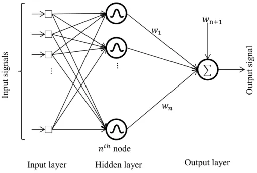
Radial Basis Functions Neural Network is another type of feed forward networks which can be used for pattern discrimination and classification, interpolation, prediction and time series problems [14]. It has the advantages of fast learning, high accuracy and strong self-adapting ability [15]. As it can be seen from Fig. 2.3, the structure of RBFNN involves three layers. The first layer is composed of input features. Each feature in the first layer is directly connected to all neurons of the hidden layer without any weight. Each neuron in the hidden layer implements one radial basis function and provides a nonlinear transformation for the input space. The Gaussian function is the most used activation function and is shown in eq. (2.5).

𝜑𝑖(𝐱, 𝐜𝑖, 𝜎𝑖) = 𝑒 −‖𝐱−𝐜𝑖‖ 2 2𝜎𝑖2 _(2.5) ... ... _... ...

Input signals _{Output s}

ignals

Hidden layer 1 Hidden layer 2 Output layer

∑ ∑ ∑ weight 𝑤_𝑖𝑗1 𝑤_𝑘𝑖2 𝑤_𝑜𝑘3 𝑖𝑡ℎ_node _𝑘𝑡ℎ_node 𝑜𝑡ℎ node +1 +1 +1

(43)

9

Where the activation of the radial basis function 𝜑_𝑖 is localized around center 𝐜_𝑖 and its localization degree is limited by 𝜎𝑖 [16], and 𝐱 is the input data sample. A localized representation of

information that is done by hidden-layer neurons helps the training process not only to reduce the output error for the current data sample 𝒙, but also to minimize disturbance to those already learned [17].

The output of the network is a linear combination of outputs from the hidden-layer nodes which is shown in eq. (2.6).

𝑦(𝐱) = 𝑤_n+1+ ∑𝑛_𝑖=1𝑤_𝑖𝜑_𝑖(𝐱) (2.6) Where 𝑛 is the number of neurons in hidden layer, 𝑤n+1 is the bias term and 𝑤𝑖 are weights for

the output linear combiner.

Fig. 2.3 Radial Basis Functions Neural Network with one hidden layer.

2.1.3 Learning Algorithms

As described in [11], there are three different points of view that can be used in categorizing learning algorithms. The first one is the mechanism that is used for learning which can be supervised, unsupervised, a combination of supervised and unsupervised and reinforcement type of learning. In supervised learning, each data sample that is fed to the learning algorithm is

... ... ∑

Input signals Output s

ignal

𝑛𝑡ℎ_node

𝑤𝑛

Hidden layer Output layer Input layer

𝑤₁

(44)

10

previously labeled by a supervisor so the learning algorithm can compare its response with the actual label. In unsupervised type of learning, the data samples are not labeled by a supervisor so the learning algorithm has to look for the similarities within the data samples and determine which of them can form a group together. There is also a possibility to combine supervised and unsupervised methods to learn the parameters of a model. An example of this approach is discussed in section 2.1.3.3 for learning the parameters of an RBFNN model. Reinforcement learning is a kind of trial and error way of learning in which the learning algorithm interacts with the environment and learns from the consequences of its previous action. The algorithm is assigned a numerical value describing the amount of its success after doing each action. In fact, the algorithm learns how to select the action which maximizes its accumulated reward points.

The second point of view classifies learning algorithms based on the time that the parameters of the system are updated. If the parameter update occurs after seeing all the data samples, the learning algorithm acts in an offline manner. On the contrary, if parameter updates happens on arrival of each new data sample, we will have an online learning.

The third aspect categorizes learning algorithms based on whether parameter updates is done in a deterministic or stochastic way. Boltzmann learning rule is an example of stochastic learning approach. Fig. 2.4 provides a schematic diagram of the taxonomy of learning algorithms from the three different points of view.

(45)

11

Fig. 2.4 A taxonomy of learning algorithms from three different points of view [11]

2.1.3.1 Supervised Learning

In supervised algorithms we need to provide both the input patterns and their corresponding desired outputs to the algorithm during the training process. The aim of the training is to infer a mapping function from the input space to the desired output space by minimizing the output error. A possible approach to minimize the output error is using the method below described.

Lear ni ng A lg or it hm s Supervised learning

Gradient descent learning Forced Hebbian/Correlative learning

Unsupervised learning

Hebbian learning Competitive learning A combination of supervised / unsupervised

learning Reinforcement learning Lear ni ng A lg or it hm Online learning Offline learning Lear ni ng A lg or it hm Deterministic learning Stochastic learning

(46)

12

2.1.3.1.1 Steepest Descent

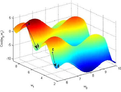
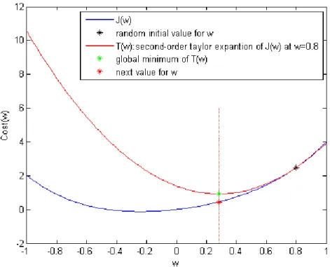
Steepest descent is a gradient descent based method. This method is one of the simplest and the most fundamental minimization methods for unconstrained optimization. Given a cost function Ω(𝑤₀, 𝑤₁, … , 𝑤_𝑛), the steepest descent method will start by initializing 𝑤₀, 𝑤₁, … , 𝑤_𝑛 to some random values and tries to minimize the cost function by updating parameters’ values through 𝑡 = 1,2, … , 𝑇 iterations. The update of parameter 𝑤_𝑘 is done by subtracting its current value from the gradient of cost function with respect to 𝑤_𝑘 as stated in eq. (2.7).

𝑤_𝑘(𝑡+1) = 𝑤_𝑘(𝑡) − 𝛼 𝜕

𝜕𝑤_𝑘(𝑡)Ω(𝑤0 (𝑡)

, 𝑤₁(𝑡), … , 𝑤_𝑛(𝑡)), 𝑘 = 0,1,2, … , 𝑛 (2.7) Where 𝛼 is the learning rate and defines the step size the algorithm is taking towards the local minima of the cost function., Gradient descent cannot guarantee finding the global minimum and the result is strongly dependent on the initial values of the parameters as can be seen in Fig. 2.5.

.

Fig. 2.5 The dependency of gradient descent on the initial parameters’ value

2.1.3.1.1.1 Back Propagation technique

For training the MLP neural network, one can use the Back Propagation (BP) technique. BP uses the steepest descent method for training process. The aim is to find linear weights 𝐰 which minimize the cost function stated in eq. (2.8).

(47)

13 Ω(𝐰) = 1 2𝑚× ∑ (y(𝐱𝑖, 𝐰) − 𝑡𝑖) 2 𝑚 𝑖=1 (2.8)

Where 𝑚 is the number of training data samples, y(𝐱𝑖, 𝐰) is the output of MLP neural network for

input data sample 𝐱_𝑖, parameterized by the weights and 𝑡_𝑖 is the target value for 𝑖𝑡ℎ_{training data}

sample. BP algorithm first initializes 𝐖 parameters with random values and continue to update these parameters until the performance of the network is satisfactory. To update the weight 𝑤_𝑎𝑏𝑙 (𝑗) (i.e., which connects neuron 𝑎 in layer 𝑙 to neuron 𝑏 in layer −1 ) in 𝑗𝑡ℎ_{iteration eq. 2.9 will be}

used.

𝑤_𝑎𝑏𝑙 (𝑗)= 𝑤_𝑎𝑏𝑙 (𝑗−1)− 𝛼 𝜕

𝜕𝑤_𝑎𝑏𝑙 (𝑗−1) Ω(𝐰) (2.9)

Where 𝛼 is the learning rate and 𝜕

𝜕𝑤_𝑎𝑏𝑙 (𝑗−1) Ω(𝐰) is the gradient of cost function with respect to 𝑤𝑎𝑏 𝑙

in (𝑗 − 1)𝑡ℎ_{iteration. The gradient value for all weights will be calculated using the following}

procedure:

Given a training example(𝐱_𝑖, 𝑡_𝑖), a “forward pass” will be run to compute all the activations throughout the network, including the output value y(𝐱_𝑖, 𝐰). Then, for each neuron in layer 𝑙, it is measured how much this neuron is responsible for any errors at the output in iteration (𝑗 − 1). It is done by calculating the error term 𝛅𝑙 (𝑗−1) _{. 𝛅}𝐿+1 (𝑗−1)_{(please remember that L is the number of}

hidden layers) which can be directly obtained by calculating the difference between the network's activation and the true target value. For the hidden units, 𝛅𝑙 (𝑗−1)_{will be computed based on a}

weighted average of the error terms of the nodes in layer 𝑙 + 1 as stated in eq. (2.10).

𝛅𝑙 (𝑗−1) = (𝐰𝑙 (𝑗−1))𝑇𝛅𝑙+1 (𝑗−1) .∗ 𝑔′(𝐳𝑙 (𝑗−1)) , 2 ≤ 𝑙 ≤ L (2.10) Where 𝐰𝑙 (𝑗−1)_{is a vector of linear weights in iteration (𝑗 − 1) which connects layer 𝑙 to layer 𝑙 −}

1; 𝑔′ is the derivative of sigmoid function 𝑔 shown in eq. 2.11 and 𝐳𝑙 (𝑗−1)_{can be calculated from}

eq. 2.12 𝑔′(𝑧) = 𝑔(𝑧)(1 − 𝑔(𝑧)) where 𝑔(𝑧) = 1 1+𝑒−𝑧 (2.11) 𝐳𝑙 (𝑗−1) = { 𝐰 1 (𝑗−1)_𝐱 𝑖 , 𝑙 = 2 𝐰𝑙−1 (𝑗−1)_𝑔(𝐳𝑙−1 (𝑗−1)_{), 3 ≤ 𝑙 ≤ L} (2.12)

(48)

14

This procedure is repeated for all data samples. The gradient of cost function with respect to each weight 𝑤_𝑎𝑏𝑙 _{in iteration (𝑗 − 1) will be obtained as stated in eq. (2.13).}

𝜕 𝜕𝑤_𝑎𝑏𝑙 (𝑗−1)Ω(𝐰) = 1 𝑚× ∑ 𝜑𝑏 𝑙 (𝑗−1) (𝐱𝑖)𝛿𝑎 𝑙+1 (𝑗−1) (𝐱𝑖) 𝑚 𝑖=1 (2.13)

Where 𝜑_𝑏𝑙 (𝑗−1)(𝐱_𝑖) is the output of neuron 𝑏 in layer 𝑙 for input pattern 𝐱_𝑖 in iteration (𝑗 − 1). 2.1.3.1.2 Newton’s Method

Steepest descent method may take a large number of iterations to converge. Newton’s method gives a much faster solution to find the parameter values for which the cost function Ω(𝐰) is minimum. Newton’s method starts by initializing 𝐰 to some random values where 𝐰 is a 𝑛 × 1 vector of parameters. It then approximates the cost function by a quadratic function in the current location using the second-order Taylor expansion. The next step is to minimize this model and obtain the next parameter values. Fig. 2.6 shows one step of Newton’s method. Eq. (2.14) states the quadratic estimation of cost function Ω(𝐰) around point 𝐰(𝑡)_{= (𝑤}

0 (𝑡) , 𝑤₁(𝑡), … , 𝑤_𝑛(𝑡)). Ω(𝐰) ≈ Ω(𝐰(𝑡)_{) + ∇} 𝐰(𝑡)× (𝐰 − 𝐰(𝑡))𝑇+ 1 2× (𝐰 − 𝐰 (𝑡)₎𝑇_𝐇(𝑡)_{(𝐰 − 𝐰}(𝑡)₎ _(2.14)

Where ∇_𝐰(𝑡) and 𝐇(𝑡) are the gradient and the second partial derivative of the cost function at point

𝐰(𝑡)_{, respectively. The second partial derivative of cost function, 𝐇}(𝑡)_{, is also called the Hessian}

matrix. The estimated function depicted in (2.14) will be minimized when eq. (2.15) is satisfied.

∇_𝐰(𝑡)+ 𝐇(𝑡)(𝐰 − 𝐰(𝑡)) = 0 (2.15)

Solving eq. (2.15) will give us the Newton’s method parameter update which can be seen in eq. (2.16).

𝐰 = 𝐰(𝑡)− (𝐇(𝑡))−1∇_𝐰(𝑡) (2.16)

For Newton's method to work, the Hessian 𝐇(𝑡)_{has to be a positive definite matrix for all 𝑡 which}

in general cannot be guaranteed [12]. Moreover, within each iteration of Newton’s method we need to calculate the inverse of Hessian matrix which is of order 𝑂(𝑛3_{), being 𝑛 the number of}

parameters. These limitations stimulated the development of alternatives to Newton’s method, the Quasi-Newton methods. These methods are general unconstrained optimization methods, and

(49)

15

therefore do not make use of the special structure of nonlinear least square problems [11]. Two other methods that exploit this structure but assume that the problem is of type non-linear least square are the Gauss-Newton and the Levenberg-Marquardt methods, which will be presented in sections Section 2.1.3.1.4 and Section 2.1.3.1.5 respectively.

Fig. 2.6 Example of one step of Newton’s method

2.1.3.1.3 Quasi -Newton methods

In quasi-Newton methods the Hessian matrix does not need to be computed. Instead, the Hessian matrix is updated by calculating the change of gradient between the current and previous iteration. There are different methods for updating Hessian matrix such as Davidson–Fletcher–Powell formula (DFP), SR1 formula (Symmetric Rank one), the BHHH method, the BFGS method and its low-memory extension, L-BFGS [18]. It is stated in [11] that BFGS update rule, shown in eq. (2.17), is the most effective for a general unconstrained method.

𝐇_{𝐵𝐹𝐺𝑆}(𝑡+1) = 𝐇(𝑡)+ (1 +(𝐪(𝑡))𝑇𝐇(𝑡)𝐪(𝑡) (𝐬(𝑡)₎𝑇_𝐪(𝑡) ) 𝐬(𝑡)(𝐬(𝑡))𝑇 (𝐬(𝑡)₎𝑇_𝐪(𝑡)− ( 𝐬(𝑡)(𝐪(𝑡))𝑇𝐇(𝑡)+𝐇(𝑡)𝐪(𝑡)(𝐬(𝑡))𝑇 (𝐬(𝑡)₎𝑇_𝐪(𝑡) ) (2.17) Where 𝐬(𝑡) _{= 𝐰}(𝑡+1)_{− 𝐰}(𝑡)_{and 𝐪}(𝑡) _{= 𝛻} 𝐰(𝑡+1) − 𝛻𝐰(𝑡).

(50)

16

2.1.3.1.4 Gauss-Newton method

Since the calculation of Hessian Matrix and its inverse can be problematic and expensive, Gauss-Newton method uses another estimation of Hessian matrix in Gauss-Newton’s update rule formula, eq. (2.16). To estimate the Hessian matrix, Gauss-Newton method assumes that the problem is a non-linear least square problem. The cost function of such problems is stated in eq. (2.18).

Ω(𝐰) =1

2∑ 𝐞𝑖 2_(𝐰) 𝑚

𝑖=1 , 𝐰 = (𝑤0, 𝑤1, … , 𝑤𝑛) (2.18)

Where 𝑚 is the number of data samples and 𝒆_𝑖(𝐰) is the error of the network parameterized by 𝐰 while feeding 𝑖𝑡ℎ _{input pattern. The elements of first-order partial derivative of Ω(𝐰) is computed}

as depicted in eq. (2.19). ∇𝑤𝑗= ∑ 𝐞𝑖 𝜕𝐞𝑖 𝜕𝒘𝑗 𝑚 𝑖=1 = ∑𝑚𝑖=1𝐞𝑖𝐉𝑖𝑗 , 𝑗 = 0,1, … , 𝑛 (2.19)

Eq. (2.20) shows the matrix notation of eq. (2.19) in 𝑡𝑡ℎ_iteration

∇_𝐰(𝑡)= (𝐉(𝑡))𝑇𝐞(𝑡) (2.20)

Where 𝐉𝑖𝑗s are the elements of Jacobean matrix 𝐉. The elements of Hessian matrix can also be

computed by eq. (2.21). 𝐇_𝑗𝑘 = ∑ (𝜕𝐞𝑖 𝜕𝐰𝑗 𝜕𝐞𝑖 𝜕𝐰𝑘+ 𝐞𝑖 𝜕2𝐞𝑖 𝜕𝐰𝑗𝜕𝐰𝑘) 𝑚 𝑖=1 , 𝑗, 𝑘 = 0,1, … , 𝑛 (2.21)

Gauss-Newton method ignores the second term in eq. (2.21) and approximate the elements of Hessian matrix as stated in eq. (2.22)

𝐇_𝑗𝑘 ≈ ∑ (𝜕𝐞𝑖 𝜕𝐰𝑗 𝜕𝐞𝑖 𝜕𝐰𝑘) = ∑ 𝐉𝑖𝑗𝐉𝑖𝑘 𝑚 𝑖=1 𝑚 𝑖=1 , 𝑗, 𝑘 = 0,1, … , 𝑛 (2.22)

Eq. (2.23) shows the matrix notation of eq. (2.22) in 𝑡𝑡ℎ_iteration.

𝐇(𝑡) _{= (𝐉}(𝑡)₎𝑇_𝐉(𝑡) _(2.23)

By replacing eqs (2.20) and (2.23) in eq. (2.16), the Gauss-Newton update rule will be obtained as depicted in eq. (2.24).

(51)

17

𝐰 = 𝐰(𝑡)_{− ((𝐉}(𝑡)₎𝑇_𝐉(𝑡)₎−1_(𝐉(𝑡)₎𝑇_𝐞(𝑡) _(2.24)

2.1.3.1.5 Levenberg-Marquardt

As previously stated, Gauss-Newton method is faster than the steepest descent but one of the problems associated with Gauss-Newton method [19] is that there is no guarantee for (𝐉(𝑡)₎𝑇_𝐉(𝑡)_to

be invertible as we need to calculate the inverse of (𝐉(𝑡)₎𝑇_𝐉(𝑡)_{in each iteration 𝑡. In order to}

guarantee that (𝐉(𝑡)₎𝑇_𝐉(𝑡)_{is invertible, it must be a nonsingular matrix. A nonsingular matrix is a}

square matrix whose determinant is nonzero. To guarantee the nonsingularity of (𝐉(𝑡)₎𝑇_𝐉(𝑡)_,

Jacobean matrix 𝐉 must have row rank 𝑛; that means the 𝑛 rows of matrix 𝐉 should be linearly independent.

Levenberg-Marquardt algorithm blends Gauss-Newton and steepest descent methods to take the advantage of Gauss-Newton speed while handling the situations at which the divergence happens. To blend the two methods, Levenberg-Marquardt introduces the update rule as shown in eq. (2.25). 𝐰 = 𝐰(𝑡)− ((𝐉(𝑡))𝑇𝐉(𝑡)+ 𝛿𝐈)−1(𝐉(𝑡))𝑇𝐞(𝑡) (2.25) Where 𝐈 is an identity matrix and 𝛿 is a scalar value. Please note that by adding diagonal matrix 𝛿𝐈 to term (𝐉(𝑡)₎𝑇_𝐉(𝑡)_{, Levenberg-Marquardt algorithm avoids rank deficiency of 𝐉 in iteration 𝑡 and}

guarantees the inevitability of term (𝐉(𝑡)₎𝑇_𝐉(𝑡)_{+ 𝛿𝐈 .}

Levenberg-Marquardt changes the value of 𝛿 based on the current situation. Considering eq. (2.25), if we set the value of 𝛿 quite small and near to zero, the effect of second-derivative elements increases and the algorithm behaves as the Gauss-Newton approach does. On the other hand, if we increase the value of 𝛿, the effect of second-derivative elements can be neglected and the algorithm follows the steepest descent approach. In this situation, Levenberg-Marquardt starts with rapid Gauss-Newton approach by assigning a small value to 𝛿.

If the error goes down following an update, it means that the quadratic assumption on Ω(𝐰) (i.e., the cost function) is valid; so we accept the new values for the parameters and continue with Gauss-Newton approach for the next iteration. The algorithm even makes 𝛿 smaller usually by a factor of 10 for the next iteration [20].

(52)

18

On the contrary, if the error goes up following an update (i.e., divergence happened maybe because of taking a very big step while we were near the minimum location so we simply jumped over the minimum), Levenberg-Marquardt resets parameters to their previous values and increases the value of 𝛿 (i.e., usually by a factor of 10 [20]) to enhance the influence of steepest descent part.

2.1.3.2 Improving the performance of the training algorithms for nonlinear least square problems by separating linear and nonlinear parameters

As stated in [21], considering a nonlinear least square problem, in order to improve the performance of the training algorithms, one can exploit the separability of the model parameters into linear and nonlinear. Suppose that 𝐮 and 𝛖 are vectors of linear and nonlinear parameters, respectively. The output of the models can be represented as eq. (2.26).

𝐲 = 𝛟(𝛖)𝐮 (2.26)

Where 𝛟 represents the output matrix of the last nonlinear hidden layer (possibly with a column of ones to consider the model output bias). When eq. (2.26) is replaced in eq. (2.18), we have:

Ω(𝐮, 𝛖) =1 2∑ 𝐞𝑖 2_{(𝐮, 𝛖)} 𝑚 𝑖=1 = ‖𝐭−𝛟(𝛖)𝐮‖22 2 (2.27)

Where 𝐭 is a vector of target values. For any value of 𝛖, the minimum of cost function Ω with respect to 𝐮 can be obtained using the least squares solutions, here determined with application of pseudo-inverse:

𝐮

̂(𝛖) = 𝛟(𝛖)+𝐭 (2.28)

By replacing eq. (2.28) in eq. (2.27) a new criterion is obtained, as shown in eq. (2.29), which only depends on the nonlinear parameters.

𝜓(𝛖) =‖𝐭−𝛟(𝛖)𝛟(𝛖)

+_𝐭‖ 2 2

2 (2.29)

To minimize eq. (2.29), its gradient with respect to 𝛖 must be computed. It can be proved [22] that the gradient of 𝜓 can be determined, computing first the optimal value of the linear parameters, using eq. (2.28), replacing this in the model, and subsequently performing the usual calculation of the gradient (only for the partition related with the nonlinear parametrs). Using the criterion stated

(53)

19

in eq. (2.29) presents some advantages, comparing with the use of the criterion depicted in eq. (2.27) [21]:

 It lowers the dimensionality of the problem;

 When the Levenberg-Marquardt is used, each iteration is computationally cheaper;

 Usually a smaller number of iterations is needed for convergence to a local minimum, since: 1. The initial value of (2.29) is much lower than the one obtained with (2.27);

2. Eq. (2.29) usually achieves a faster rate of convergence than (2.27).

2.1.3.3 Three learning strategies for training RBFNN

There are three different learning strategies to determine the parameters of a RBF neural network, depending on the approach that is considered for determining the centers and spreads of the radial-basis functions of the network [12, 23, 24].

In one approach, the centers can be selected from the training data set in a random manner. The spreads can then be calculated using eq. (2.30) [25].

𝜎 = 𝑑𝑚𝑎𝑥

√2𝑛 (2.30)

Where 𝑑_𝑚𝑎𝑥 is the maximum Euclidean distance between centers and 𝑛 is the number of centers. If the training data are distributed in a representative manner for the problem at hand, this could be a wise approach. The linear parameters 𝐮 = [𝑢₁, 𝑢₂, ⋯ , 𝑢_𝑛, 𝛼₀] are then found using eq. (2.31).

𝐮 = ∅+𝐭 (2.31)

Where 𝐭 is a vector of target values and ∅+_{is the pseudo-inverse of the hidden neurons’ output}

matrix.

Another approach is a combination of supervised and unsupervised methods which is also called self-organized selection of centers. In this approach, the locations of the centers are found by a clustering technique like k-means clustering (please see Algorithm 2.1).