Fiscal reform and government debt in Japan: a neoclassical perspective

.

...

Fiscal Reform and Government Debt in

Japan: A Neoclassical Perspective

Gary Hansen (UCLA) and Selo ˙Imrohoro˘glu (USC)

Table of Contents

Basic Issue

Two significant challenges faced by Japan

High debt to output ratio (close to 150%).

Projected increase in government expenditures due to aging population.

Spending to output projected to rise by 7% due to increases in pension and health spending.

We explore size and consequences of fiscal responses to this problem.

High Debt

Aging Population

Implications of Aging Population

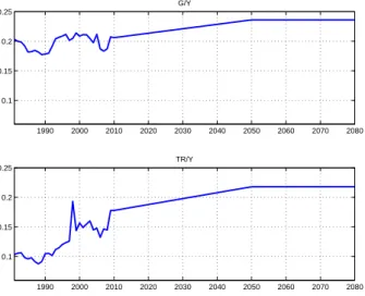
Fukawa and Sato (2009)

1990 2000 2010 2020 2030 2040 2050 2060 2070 2080 0.1 0.15 0.2 0.25 G/Y 1990 2000 2010 2020 2030 2040 2050 2060 2070 2080 0.1 0.15 0.2 0.25 TR/Y

What We Do

Formulate and calibrate neoclassical growth model of Japan.

Calculate effects of alternative fiscal policies designed to achieve fiscal balance.

How large must tax rates on labor and/or consumption be to achieve this goal?

First consider reducing transfers (lump taxes) and then consider distorting taxes.

What We Do

Hayashi and Prescott (2002) and Chen, ˙Imrohoro˘glu and ˙Imrohoro˘glu (2006).

Economic agents have perfect foresight.

Characterize how model performs from 1981-2010.

Take as exogenous TFP, tax rates, government consumption, transfers and population.

Use observed values 1981-2010.

Use model to forecast from 2011 and beyond.

Government projections for population to 2050. Forecasts of Fukawa and Sato (2009) of G/Y and

Features of Model

Government debt is introduced with bond price (interest rate) endogenous.

Government bonds enter utility function⇒ rate of return dominance.

Endogenous labor choice⇒ consumption and labor income taxes are distorting.

“Fiscal Sustainability Rule” insures that intertemporal government budget constraint is satisfied.

Related Literature

˙Imrohoro˘glu and Sudo, “Productivity and Fiscal Policy in Japan: Short Term Forecasts from the Standard Growth Model”

Experiment with policies to eliminate budget deficit in near future by increasing consumption tax.

˙Imrohoro˘glu and Sudo, “Will a Growth Miracle Reduce Debt in Japan”

Assess possibility that high TFP growth could eliminate government debt.

Model: Government Budget

Gt +TRt∗+Bt = ηtqtBt+1+τc,tCt+τh,tWtht

+τk,t(rt −δ)Kt +τb,t(1−qt−1)Bt.

ιt =

{

1 if Bs/Ys ≥bmax for some s ≤t,

0 otherwise

Dt =κιt(Bt −Bt),

Model: Household’s Problem

∑

Model: Firm’s Problem

NtYt = At(NtKt)θ(Ntht)1−θ

Nt+1Kt+1 = (1−δ)NtKt +NtXt

Stationary Equilibrium Conditions

Given a per capita variable Zt we obtain its detrended

counterpart

zt =

Zt

A1/_t (1−θ) .

First order conditions and market clearing conditions combine to give 10 equations in 10 unknowns

{ct, xt, ht, yt, kt+1, bt+1, dt, qt, wt, rt} for each period t.

Computation Objective: Find value for k1 such that

Population and Labor Input

Nt =working age population between the ages of 20 and

69

Use actual values for 1981-2010 Use official projections for 2011-2050 Population constant after 2050

ht is employment per working age population multiplied

by average weekly hours worked divided by 98 (discretionary hours available per week).

National Accounts: Hayashi and Prescott (2002)

Table : Adjustments to National Account Measurements

C = Private Consumption Expenditures I = Private Gross Investment

+ Change in Inventories + Net Exports

+ Net Factor Payments from Abroad G = Government Final Consumption Expenditures

+ General Government Gross Capital Formation + Government Net Land Purchases

−Book Value Depreciation of Government Capital Y = C +I +G

Government Accounts

Public health expenditures in Japan are included in Gt.

TRt, includes social benefits (other than those in kind,

which are in Gt,) that are mostly public pensions, plus

other current net transfers minus net indirect taxes. 8.1% of output is added to TRt since modeling of flat tax

Tax Rates

τh,t, are average marginal labor income tax rates

estimated by Gunji and Miyazaki (2011).

Last value is 0.324 for 2007 and we assume that this remains constant thereafter.

τk,t, is constructed following methodology in Hayashi and

Prescott (2002).

Last value is 0.3557 for 2010 and we assume that this remains constant thereafter.

Tax Rates, continued

Tax Rate on Consumption, τc,t

0% 1981-1988 3% 1989-1996 5% 1997-2013 8% 2014

10% 2015 and beyond.

Tax Rates, continued

Consumption Tax Rate Labor Income Tax Rate Capital Income Tax Rate

Technology Parameters

At =Yt/(Ktθh1t−θ).

θ =0.378, which is the average value from 1981-2010. γt =At+1/At, comes from the actual data between

1981 and 2010.

γt =1.0151−θ. for 2011 and beyond.

Preference Parameters

Five preference parameters, β, α, ψ, ϕ, and µ. µ =µt/A1/t (1−θ) =1.1.

ψ=0.5, the Frisch elasticity of labor supply estimated by Chetty et al (2012).

Preference Parameters, continued

For β, α, and ϕ, use equilibrium conditions to obtain a value for each year, and then average over the sample:

βt = (1+τc,t+1)γ1/ (1−θ) t ct+1 (1+τc,t)ct [ 1+ (1−τk,t+1) ( θyt+1 kt+1 −δ )] αt = h_t−1/ψ(1−τ_h,t)(1−θ)yt (1+τc,t)ctht ϕt =ηt(µ+bt+1) [ qtγ 1/(1−θ) t (1+τ )c − βt[1− (1−qt)τb,t+1] (1+τ )c ] .

Bond Price

Need empirical counterpart to qt :

qt =

Bt+1/Ft

(Bt+1+Pt+1)/Ft+1

.

Bt is beginning of period debt.

Pt is interest payments made in period t.

Bond Price, continued

Bond Price, continued

Before Tax Rate of Return on Bonds Before Tax Rate of Return on Capital

1980 1985 1990 1995 2000 2005 2010 0.02

0.04 0.06 0.08

After Tax Rate of Return on Bonds After Tax Rate of Return on Capital

Structural Parameters

Table : Calibration of Structural Parameters

Parameter Value θ 0.3783 Data Average δ 0.0842 Data Average β 0.9677 FOC, 1981-2010 α 22.6331 FOC, 1981-2010 ψ 0.5 Chetty et al (2012) ϕ 0.063 FOC, 1981-2010 µ 1.1 fit qt for 1981-2010

Fiscal Sustainability

dt =κιt(bt −b y),

ιt =

{

1 if Bs/Ys ≥bmax for some s ≤t,

0 otherwise

b=0.6

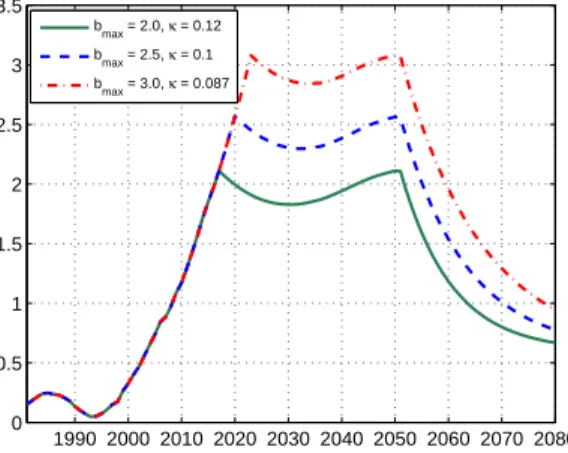
Consider bmax = 200%, 250% and 300%.

Japan already near 150%.

Fiscal Sustainability

1990 2000 2010 2020 2030 2040 2050 2060 2070 2080 0

2 4

Debt to GNP Ratio, b_max = 2.5

1990 2000 2010 2020 2030 2040 2050 2060 2070 2080 0

0.2 0.4 0.6

Consumption Tax Equivalent Revenue Requirement, b max = 2.5 κ = 0.05

κ = 0.1 κ = 0.15

Fiscal Sustainability

Figure : Bond to Output Ratio for Alternative Maximum Debt to GNP Ratios

Fiscal Sustainability

Comparison of Benchmark with Data

Comparison of Benchmark with Data

Comparison of Benchmark with Data

Government Finance in Steady State

consumption tax rate

G + TR divided by benchmark output Revenue

divided by benchmark output

Government Finance in Steady State

labor income tax rate Revenue divided by benchmark output G + TR divided by benchmark output

Tax Wedge

From first order condition for labor, can define

1−τt ≡ 1₁−₊τ_τh,t_c,t

⇒τt = τc,t

+τh,t 1+τc,t

Government Finance in Steady State

labor income tax rate

consumption tax rate

Effective tax rate

Implementation of Tax Increases

τx ,t =

  

τx ,last if Bs/Ys ≤bmax for all s ≤t

τx +π if Bs/Ys >bmax for some s ≤t and Bt/Yt >b

τx if Bt/Yt ≤b.

where x =c or h and t ≥2015.

π is chosen as the smallest increment that leads to the activation of the second trigger (convergence to steady state).

Increase Consumption Tax Only

Consumption Tax Experiment 1

labor income tax rate consumption tax rate

Increase Both Consumption and Labor Tax

Use Consumption Tax to Retire Debt, Increase Labor Tax to 45%.

19800 2000 2020 2040 2060 2080 2100 0.1 0.2 0.3 0.4 0.5 0.6 0.7

Consumption Tax Experiment 2

consumption tax rate

Increase Both Consumption and Labor Tax

Use Labor Tax to Retire Debt, Increase Consumption Tax to 40%.

19800 2000 2020 2040 2060 2080 2100 0.1 0.2 0.3 0.4 0.5 0.6 0.7

Labor Income Tax Rate Experiment

labor income tax rate

consumption tax rate

Transition Paths for Various Experiments

Transition Paths for Various Experiments

Transition Paths for Various Experiments

Effective Tax Distortion

Conclusion

Soaring debt to GNP ratio implies fiscal “day of reckoning” is soon–around 2020.

Costs of aging population require large nearly permanent increases in tax rates:

Consumption tax: permanent increase to 48% with additional 12% during transition.

Both consumption and labor tax: permanent increase to 40%, smaller additional increase during transition.

Conclusion

Other options to explore:

Broaden tax base: 8.1% of GNP potential. Social security and health insurance reform. Increase fertility and/or allow immigration. Encourage female labor force participation. Reduce spending.