António Afonso, Raquel Balhote
Interactions between Monetary Policy
and Fiscal Policy
WP13/2014/DE/UECE _________________________________________________________
De pa rtme nt o f Ec o no mic s
W
ORKINGP
APERS1
Interactions between Monetary Policy
and Fiscal Policy
*
António Afonso
$, Raquel Balhote
#September 2014
Abstract
Using a panel data set of 14 EU countries from 1970 to 2012, we study the type of monetary and fiscal policies of both authorities, and assess how they are influenced by certain economic variables and events (the Maastricht Treaty, the Stability and Growth Pact, the Euro and crises). Results show that inflation has a significant impact on monetary policy, and that governments raise their primary balances when facing increases in debt. Another goal is to characterise the type of interactions established between central banks and national governments, i.e. if their policies complement one another, or whether there is a more dominant one. Still, our results point to the lack of
evidence concerning central banks’ response to fiscal policy.
JEL: E52, E62, E63, H62.
Keywords: interactions, monetary policy, fiscal policy, reaction functions.
*
The authors are grateful to Luís Martins for valuable comments. The opinions expressed herein are those of the authors and do not necessarily reflect those of their employers.
$
ISEG/ULisbon – University of Lisbon, Department of Economics; UECE – Research Unit on Complexity and Economics, R. Miguel Lupi 20, 1249-078, Lisbon, Portugal, email: aafonso@iseg.utl.pt. UECE is supported by the Fundação para a Ciência e a Tecnologia (The Portuguese Foundation for Science and Technology) through the Pest-OE/EGE/UI0436/2011 project. European Central Bank, Directorate General Economics, Kaiserstraße 29, D-60311Frankfurt am Main, Germany.
#
ISEG/ULisbon – University of Lisbon, R. Miguel Lupi 20, 1249-078 Lisbon, Portugal. email:
2 1. Introduction
On the 7th of February 1992, the Maastricht Treaty was signed, which was the first step towards a common currency among the member states of the European Union (EU). This treaty was established following convergence criteria which each member state was obliged to comply with, based on rules on budget deficit and debt levels, low inflation and interest rates close to the EU average. Thus, it contributed towards achieving price stability and fiscal sustainability.
However, these Maastricht provisions did not seem to be sufficient enough to deal with excessive deficits, which led to the formation of other procedures to complement the creation of the Economic and Monetary Union (EMU). In 1997, members from the EU agreed to the Stability and Growth Pact (SGP), a set of fiscal rules for maintaining and reinforcing low budget deficits, whereby annual government budget deficit and government debt may not exceed 3% and 60% of GDP, respectively. Finally, the third stage of the EMU took place on the 1st of January 1999, with the launch of a common single currency, the Euro, which was to be used as the monetary unit for all transactions by January 2002.
Despite all the advantages that these three economic milestones brought about, they restricted the use of fiscal policy, especially when countries joined the Euro area, lost their individual monetary policy, and became aligned to a common monetary policy. This leads us to need to think about the relationship created between a country’s fiscal and monetary policies.
The interactions between fiscal policy and monetary policy are a complex topic to study, as the role of each authority has a different impact on the economy, which could be the reason why equilibrium under these two policies is similarly difficult to determine. Thus, the type of relationship established by both authorities is important in determining how their policies will influence the levels of inflation, debt and economic growth, in other words, all the aspects that are related to the economic performance of a country.
3
Maastricht Treaty, the SGP, the Euro and crises have influenced monetary and fiscal policies.
For a sample of 14 European countries during the period of 1970-2012, we performed a panel data analysis, which took into account the impact that these policies have on all of the countries, on average. Our results show that inflation is quite relevant for monetary policy, and that primary balance reacts positively to increases in government debt. Moreover, our results point to the lack of evidence concerning central
banks’ response to fiscal policy.
Furthermore, in relation to these events, the estimation results are all statistically significant for monetary and fiscal policies, but the dummy for the Maastricht Treaty shows that it has the biggest impact on monetary policy, probably due to the convergence criteria. On the other hand, the introduction of the Euro has a greater
negative effect on fiscal policy, together with that of a rise in countries’ budget deficits.
As we expected, crises influence monetary and fiscal policies negatively, but this effect is smoothed out if countries belong to the Euro area. In addition, we also made individual analyses for each country.
The paper is structured as follows: Section 2 provides a brief theoretical and empirical analysis of the background literature, emphasising the different policies and the degree of economic coordination; Section 3 explains the empirical specifications, namely the data and variables used in the model, as well as the econometric approaches chosen; Section 4 details the regressions that were estimated, as well as the empirical results; Section 5 summarises the conclusions.
2. Literature and Theoretical Background
2.1. Different Policies and Economic Coordination
Since the beginning of the 1980s, discussion regarding the roles of central banks and governments, as well as the relationship between monetary and fiscal authorities, started to gain more relevance. Although there is a separation of responsibilities – central banks are focused on inflation, whereas governments are concerned with cyclical conditions and the level of government indebtedness – both inflation and cyclical conditions depend on policy coordination, which means that monetary and fiscal policies depend on each other (Wyplosz, 1999).
4
Wallace (1981) argued that both authorities could be relevant in a “dominant” way.
When monetary policy dominates fiscal policy, the monetary authority can permanently control inflation, as it is free to set the level for base money. However, if fiscal policy dominates monetary policy then the monetary authority loses some of its influence in controlling inflation, and since budget deficits cannot only be financed by the issue of new bonds, then the monetary authority has to print money and address the additional problem of inflation.
Aiyagari and Gertler (1985) introduced the distinction between Ricardian and Ricardian regimes, which characterises the behaviour of a government. In a non-Ricardian regime, primary budget balances are freely set by the government and prices
are endogenously determined from the government’s budget constraints. Hence, the
fiscal authority does not commit to completely financing debt through future taxes, thus leading to monetary financing. In a Ricardian regime, the monetary authority determines the stock of money and the price level, and the government has to achieve a certain degree of primary budget surplus in order for the budget constraint to be consistent with the repayment of the initial stock of debt and to ensure fiscal solvency.
According to Leeper (1991), fiscal policy could be “active” or “passive”,
depending on the effect it will have when facing a government debt shock. An active authority discards the state of government debt and independently establishes a decision rule that depends on past, current and future variables. On the other hand, a passive
authority’s decision rule depends on the current state of government debt once it has
been constrained by the active authority’s actions and by the private optimisation.
Taylor (1993) further addressed the estimation of policy reaction function by initially proposing a monetary policy rule to control inflation for the U.S. in the early 1990s:
*) (
*) (
* y y
r
r . (1)
5
GDP, its aim is to allow central banks to be successful in stabilising inflation and output gap. Later on, after the establishment of the EMU, many authors concluded that the Taylor rule is a useful tool for conducting monetary policy in the Union and that it provides a similar level of macroeconomic stabilisation, when compared with the optimal rule (Gerlach and Schnabel, 2000).
On the other hand, when dealing with fiscal issues, the key player is the government. Based on its intertemporal budget constraint and assuming the necessary and sufficient transversality condition, the government must determine a sustainable fiscal rule in the medium and long term:1
1
1
bt dt rtbt , (2)
where bt is the public debt in year t, rt is the real interest rate in t, rtbt1 are the interest payments at the beginning of fiscal year t-1, and dt1 gt1t1st1 is the ratio of the
government primary balance to GDP generated during t-1, in which g is the government expenditure net of interest, are the tax revenues net of transfers and s denotes the real revenues from seigniorage, assumed to be constant. In equation (2), and knowing that the primary balance can be a deficit or a surplus, the change in the public debt-to-GDP ratio must cover not only the primary balance to GDP ratio but also interest payments.
2.2. Previous Empirical Evidence
The reading of the available empirical literature shows that, several authors focussed either on the monetary or on the fiscal side, on the interactions between them,
or on their impact on a country’s economy.
Concerning the study of fiscal policy and its sustainability, the studies looked essentially at two main indicators: debt and primary balance. In Bohn (1998), the U.S. primary budget surplus turned out to be an increasing function and it responded positively to the debt-to-GDP ratio, which shows that U.S. fiscal policy satisfies an intertemporal budget constraint, in a Ricardian fashion. Galí and Perotti (2003) study how the Maastricht Treaty and the SGP changed the fiscal policy in EMU countries by
1
6
making them more procyclical, and they also detect a decrease in cyclically primary deficits when facing an increase in debt. On the other hand, Afonso (2005) uses causality tests between the primary balance and government debt ratios. The results of the various tests show that for all the sub-periods (pre- and post-Maastricht Treaty and SGP periods) between 1970 and 2003, the 15 EU governments raised the primary budget surpluses as a result of increases in the outstanding stock of government debt, and they appears to use primary budget surpluses to reduce the debt-to-GDP ratio. Therefore, we can acknowledge an evidence of Ricardian fiscal regime in these papers.
Moving to monetary policy, it can be observed that reaction functions are usually based on interest rates. Altavilla (2003) estimates several reaction functions2 in order to assess how the European Central Bank (ECB) should control interest rates when facing a change in real output, inflation or the exchange rate. The conclusions are that: 1) central bank behaviour is better explained by adding a lagged interest rate and also future inflation movements; 2) the ECB should focus on simple monetary rules, as this increases the transparency and the credibility of the institution itself. Ruth (2007) develops a panel reaction function based on the Taylor rule for analysing the European
monetary policy, namely, interest rate setting since 1999. Regarding the good’s interest
rate path, in the short-term, the author only finds deviation by the ECB in cases of area-wide inflation. Clausen and Hayo (2002) also find asymmetric monetary policy effects over the short- and medium-term for Germany, Italy and France.
Furthermore, besides just measuring an interest rate reaction function for 8 major EMU countries between 1980 and 1998, Huchet’s (2003) main goal is to determine whether common monetary policy shocks induce asymmetric reactions on the
real economic activity of each country. His conclusion is that “(...) a common change
of monetary policy in all countries can lead to asymmetric reactions because these
countries still have different national structures”.
To study the interactions between monetary and fiscal policies, Leeper and Davig (2009) estimate Markov-switching policy rules for the United States. The paper’s results highlight that the impacts of a fiscal stimulus cannot be understood without studying monetary and fiscal policies jointly, since they fluctuate between active and passive behaviour. A similar approach is provided by Afonso and Toffano (2013) who report for the UK “active” and “passive” fiscal regimes in a clearer cut way, while in
2
7
Germany fiscal regimes have been overall less active, supporting more fiscal sustainability. For Italy, a more passive fiscal behaviour is uncovered in the run-up to EMU.
3. Empirical Specifications
3.1. Data and Variables
For the time period between 1970 and 2012 (43 years of annual observations), our dataset is based on 14 EU countries, where 11 belong to the Euro area3 – Austria (AT), Belgium (BE), Finland (FI), France (FR), Germany (DE), Greece (GR), Ireland (IE), Italy (IT), the Netherlands (NL), Portugal (PT) and Spain (ES) – and the other 3 are not part of the Euro area – Denmark (DK), Sweden (SE) and the United Kingdom (UK).
The variables used in the analysis are from several sources. From the European Commission AMECO database we gathered data regarding cyclically adjusted primary balance (capb), debt-to-GDP ratio (debt), nominal short-term interest rate (interest) and output gap between actual and potential gross domestic product (output gap); from the World Development Indicators (WDI) we obtained inflation (inflation); from the Financial Development and Structure dataset of the World Bank we collected M3 data, also referred to as liquid liabilities (m3). Table 1 presents the descriptive statistics for the full sample.
Table 1
Descriptive Statistics (full sample): 1970 - 2012
Mean Std. Dev. Minimum Maximum Observations capb
(% of GDP) 0.963 3.354
-25.033
(IE, 2010)
10.457
(DK, 1986) 447
debt
(% of GDP) 58.451 29.162
6.147
(FI, 1974)
170.306
(GR, 2011) 565
interest rate
(%) 7.515 4.996
0.570
(PT, 2012)
24.560
(GR, 1994) 572
output gap
(% of potential GDP) 0.089 2.350
-11.915
(GR, 2012)
7.709
(PT, 1972) 581
inflation
(annual %) 5.813 5.583
-4.480
(IE, 2009)
28.783
(PT, 1984) 561
m3
(% of GDP) 69.512 26.540
6.865
(IE, 1981)
180.332
(UK,2009) 543
3
8
To assess the impact of certain events on authorities’ policies, we have created
several dummy variables and included them in the regressions:
dmt: dummy for the Maastricht Treaty, assuming a value of 1 in the years of and after the approval of the Treaty4, and 0 otherwise;
dsgp: dummy for the adoption of the SGP framework, taking the value 1 for 1997 and subsequent years, and 0 elsewhere;
dez: dummy for countries in the Euro area, being 1 for the year of and after they became Euro area countries5, and 0 for Denmark, Sweden and the United Kingdom, since they have not adopted the Euro.
Although we do not consider this as a dummy variable, we also want to study the effect a crisis can have on monetary and fiscal policies. Therefore, from the database6 of Reinhart and Rogoff (2009), we collected data regarding the total number of crises a country had in each year (crisis). In this dataset, the types of crises are banking, currency, inflation and stock market crises, which assume the character of a dummy variable in further tests (e.g. 1, if in year t country i had a banking crisis, and 0 otherwise).
3.2. Econometric Approach
We use a panel data approach, as it notably provides the possibility of obtaining a larger sample. The general linear model is the foundation of linear panel model estimation, which is why we can estimate the parameters using the Ordinary Least Squares (OLS) method. This method is associated with three basic assumptions: exogenous covariates, uncorrelated and homoscedastic errors. However, if they do not hold, OLS estimates are biased and/or inefficient. Plus, OLS bias could also be due to endogeneity whenever there are, for instance, omitted variables or measurement errors in the covariates. To address this problem we use two conventional regression based strategies: the fixed effects model and the two stage least squares (2SLS).
According to Wooldridge (2009), the fixed effects method allows for not only the estimation of panel data models with unobserved effects, as it is efficient when
4
The dates of the Maastricht referendum approval are different for each country: 1992 for Belgium, France, Greece, Ireland, Italy, the Netherlands, Portugal and Spain; 1993 for Denmark, Germany and the United Kingdom; 1994 for Austria, Finland and Sweden.
5
The date of entry is different among countries: 1999 for Austria, Belgium, Finland, France, Germany, Ireland, Italy, the Netherlands, Portugal and Spain; 2001 for Greece.
6
9
idiosyncratic errors are uncorrelated and homoscedastic, but also for the estimation of unbalanced panels, i.e., when the sample is missing years for some cross-sectional units.
Additionally, although the random effects method is more efficient when the unobserved effect is uncorrelated with all the explanatory variables, fixed effects is more useful to estimate ceteris paribus effects. However, it is possible to perform the Hausman test to verify which of both methods is the most appropriate, with random effects being the null-hypothesis. Therefore, rejecting the null-hypothesis proves evidence in favour of fixed effects. For our work, this same test indicates the use of random-effects for monetary policy, as well as for the reaction function of central banks, and the use of fixed-effects for fiscal policy and the reaction function of national governments.
The third method we use is the 2SLS, to allow for instrumental variable estimations. By enabling the use of instrumental variables – exogenous variables, totally uncorrelated with the error term and partially correlated with the explanatory variables – besides the existing explanatory variables, this method also estimates ceteris paribus effects. Therefore, it solves the endogeneity problem and leads to a consistent estimator when there are omitted variables. The advantage is that, if those instrumental variables are not poor, then they may very well satisfy the two properties mentioned above; 2SLS clearly becomes a more suitable method than OLS. In our 2SLS estimations, we generally used the lagged values of explanatory variables as instrumental variables.
OLS, OLS-Fixed Effects (OLS-FE) and 2SLS are the three panel data methods considered in the estimation of our regressions, and in all of them, we apply the White diagonal covariance matrix in order to assume residual heteroscedasticity.
10 4. Empirical Analysis
4.1. Policies of the Authorities
4.1.1. Monetary Policy
In our study, as well as in the majority of the literature who follows the Taylor rule, the instrument of monetary policy used is the interest rate. Regarding the explanatory variables, for instance, Huchet (2003) uses the lagged short-term interest rate, the inflation gap and the M3 growth gap compared to its 2% target and a 4.5% reference value, respectively, and also the output gap. Altavilla (2003) creates instrument rules which vary between inflation, output gap and interest rate, and their lagged values and an autoregressive term.
Therefore, we have set up our monetary policy regression for country i (i=1,..., N) at time t (t=1,..., T) in the following form:
it it it
it it
i
it interest inflation outputgap m3 u
interest 1 1 1 1 , (3)
where interestit and interestit1are the nominal short-term interest rate at times t and t-1, inflationit1 represents inflation in period t-1, outputgapit1 is the gap in t-1, m3it1 is
the monetary aggregate M3 at time t-1,i represents the estimated individual effects for each country and uit are the independent disturbances across countries
In Table 2 we present the estimated results for regression (3) and, as expected, the short-term interest rate is sensitive to inflation (0), to the output gap ( 0) and to M3 ( 0). The estimation is conducted based on three methods, OLS, OLS-FE and 2SLS.7 The results display statistically significance in all variables, with the correct signs.
Apart from the larger impact of the lagged short-term interest rate, which softens interest rate fluctuations, inflation is the next most important variable in terms of influence on the instrument of monetary policy. The results show that a 1% increase in inflation leads to a raise of 0.165% in the nominal short-term interest rate, in order to reduce money supply, which will eventually lead to a decrease in inflation. Thus the stabilisation of the price level is in place. Clearly, sustainable economic growth is in the background, which is represented by the low positive effect that output gap has on
7
11
interest rates. This also stresses the adversarial relationship mentioned earlier between sustainable economic growth and a stable level of prices. Looking at the results in more detail, a negative relation between interest rate and M3 is clear. Perhaps this could mean that if central banks want to increase M3, they should reduce interest rates in order to
not jeopardise M3’s reference value.
Table 2
Estimation of monetary policy with interestit as dependent variable: 1970-2012
Method OLS OLS-FE 2SLS
c 1.190*** (0.343) 1.315*** (0.416) 1.226*** (0.384)
1
it
interest 0.789***
(0.029)
0.784*** (0.029)
0.790*** (0.034)
1
it
inflation 0.162***
(0.027)
0.165*** (0.029)
0.165*** (0.031)
1
it
outputgap 0.093**
(0.037)
0.090** (0.037)
0.098*** (0.038)
1
it
m3 -0.010***
(0.003)
-0.012*** (0.004)
-0.011*** (0.004)
Obs 513 513 497
2
R 0.879 0.880 0.879
Adj. 2
R 0.878 0.876 0.878
D-W stat 2.055 2.057 2.067
Hausman prob 0.9232 - 0.9567
Notes: *, ** and *** represent statistical significance at 10%, 5% and 1% levels, respectively. The robust standard errors are in brackets. Obs represents the total number of observations. D-W stat is the Durbin-Watson statistic. Hausman prob refers to the probability reached in the Hausman test.
Applying the SUR model in regression (3), formed by a system of 14 equations related to each country individually, we were able to estimate their monetary policies and thus carry out a more careful analysis through the results displayed in Table 3.
Denmark, Finland, France, Spain and Sweden are the only countries that follow the usual pattern: inflation is statistically significant and there are expected signs for all coefficients. Some other countries either do not display the expected sign or inflation seems to be less of a priority goal. For instance, whenever inflation is not significant, cyclical conditions or M3 levels assume a more relevant role: in Austria and in the United Kingdom, the major responses being to the levels of output (if they approach the potential level) and to the values established for M3, since both significantly influence short-term interest rates. On the other hand, in Ireland and in the Netherlands interest rates are only affected by M3 and output gap levels, respectively.
12 Table 3
SUR estimation of monetary policy with interestit as dependent variable: 1970-2012 Countries c interestit1 inflationit1 outputgapit1 m3it1 Obs R2
Austria 4.988***
(1.518) 0.582*** (0.078) -0.083 (0.107) 0.248** (0.109) -0.033***
(0.016) 40 0.674
Belgium 2.989*** (1.146) 0.600*** (0.078) (0.074) 0.116 -5.71E-05 (0.106) (0.011) -0.016 40 0.756
Denmark 2.163
(2.070) 0.689*** (0.083) 0.188** (0.091) 0.117 (0.106) -0.016
(0.030) 42 0.827
Finland 4.280*** (1.577) 0.684*** (0.056) (0.062) 0.118* (0.059) 0.083 -0.052* (0.027) 42 0.865
France 3.216***
(1.060) 0.570*** (0.071) 0.175*** (0.064) 0.071 (0.082) -0.020
(0.015) 42 0.766
Germany (1.608) 2.582 0.723*** (0.253) (0.316) -0.356 (0.147) 0.124 (0.012) -0.012 20 0.683
Greece -2.899
(2.728) 0.818*** (0.089) 0.245*** (0.071) 0.177 (0.151) 0.029
(0.029) 32 0.930
Ireland 4.869*** (1.039) 0.598*** (0.076) (0.051) 0.011 (0.075) 0.080 -0.035*** (0.010) 41 0.852
Italy 3.482***
(1.240) 0.575*** (0.068) 0.268*** (0.067) -0.061 (0.137) -0.026
(0.019) 42 0.841
Netherlands 3.398*** (0.773) 0.462*** (0.073) (0.069) 0.004 0.205** (0.084) (0.007) -0.011 42 0.598
Portugal 0.366
(1.092) 0.764*** (0.047) 0.164*** (0.035) 0.001 (0.063) 0.001
(0.012) 42 0.943
Spain (1.525) 2.983* 0.616*** (0.090) 0.271*** (0.075) (0.122) 0.034 (0.012) -0.018 35 0.896
Sweden (1.500) 2.116 0.650*** (0.112) (0.143) 0.273* (0.135) 0.072 (0.025) -0.015 30 0.851
United Kingdom 5.214*** (1.239) 0.421*** (0.144) 0.265 (0.219) 0.391*** (0.391) -0.024***
(0.008) 23 0.861 Notes: *, ** and *** represent statistical significance at 10%, 5% and 1% levels, respectively. The robust standard errors are in brackets. Obs represents the total number of observations. SUR linear estimation after one-step weighting matrix; total system with 513 observations.
4.1.2. Fiscal Policy
13
The fiscal policy regression we follow is notably presented by Afonso (2005), and is a simple linear dynamic model:
it it it
i
it capb debt u
capb 1 1 , (4)
where the cyclically-adjusted primary balance of country i at year t (capbit) depends on its previous observation (capbit1) and on the debt-to-GDP ratio of year t-1 (debtit1).
Bearing this in mind, the hypothesis we want to test is 0, meaning that the expected result is a positive reaction of the primary balance to changes in government debt. Table 4 reports the outcomes for fiscal policy reaction function (4), and as the estimated coefficient for debt is statistically significant we cannot reject this hypothesis.
Table 4
Estimation of fiscal policy with capbit as dependent variable: 1970-2012
Method OLS OLS-FE 2SLS
c -0.491***
(0.226)
-1.448*** (0.312)
-1.636*** (0.354)
1
it
capb 0.822***
(0.074)
0.741*** (0.089)
0.729*** (0.072)
1
it
debt 0.011***
(0.003)
0.027*** (0.005)
0.030*** (0.005)
Obs 428 428 414
2
R 0.678 0.703 0.701
Adj. 2
R 0.677 0.693 0.690
D-W stat 2.036 2.012 2.028
Hausman prob 0.0000 - 0.000
Notes: *, ** and *** represent statistical significance at 10%, 5% and 1% levels, respectively. The robust standard errors are in brackets. Obs represents the total number of observations. D-W stat is the Durbin-Watson statistic. Hausman prob refers to the probability reached in the Hausman test.
14
Subsequently, we have estimated the fiscal policy reaction functions in each country separately, using the SUR model. Table 5 shows the results.
Table 5
SUR estimation of fiscal policy with capbit as dependent variable: 1970-2012
Countries c capbit1 debtit1 Obs R2
Austria -1.604**
(0.753)
0.228* (0.136)
0.033**
(0.013) 36 0.314
Belgium -2.893*** (0.861) 0.716*** (0.077) 0.034*** (0.009) 42 0.827
Denmark -0.367
(0.464)
0.774*** (0.076)
0.025***
(0.009) 41 0.760
Finland (0.857) 1.440* 0.715*** (0.105) (0.016) -0.009 35 0.610
France 0.098
(0.346)
0.572*** (0.125)
-0.008
(0.008) 34 0.507
Germany -4,155** (1.758) (0.156) 0.053 0.074** (0.029) 21 0.170
Greece -2.744
(1.867)
0.671*** (0.108)
0.027
(0.018) 24 0.588
Ireland (1.769) -2.488 0.624*** (0.114) (0.023) 0.040* 27 0.550
Italy -5.683***
(1.716)
0.636*** (0.103)
0.059***
(0.017) 32 0.865
Netherlands (0.779) -0.786 0.619*** (0.097) (0.013) 0.021 37 0.540
Portugal -2.446**
(0.998)
0.510*** (0.119)
0.035**
(0.017) 35 0.294
Spain -4.173** (1.877) 0.994*** (0.119) 0.075** (0.034) 17 0.766
Sweden -0.369
(1.118)
0.572*** (0.100)
0.030*
(0.018) 19 0.586
United Kingdom -2.764*** (0.975) 0.934*** (0.084) 0.059*** (0.021) 26 0.742
Notes: *, ** and *** represent statistical significance at 10%, 5% and 1% levels, respectively. The robust standard errors are in brackets. Obs represents the total number of observations. SUR linear estimation after one-step weighting matrix; total system with 428 observations.
Austria, Belgium, Denmark, Germany, Ireland, Italy, Portugal, Spain, Sweden and the United Kingdom have governments that follow Ricardian fiscal regimes: debt is statistically significant and whenever it increases, primary budget surplus is raised in order to stabilise the financial situation. This pattern is also pursued by Greece and the Netherlands, although debt does not show up as being significant.
15
4.2. Interactions between Monetary and Fiscal Authorities
Besides estimating the policies of each authority, we have also decided to include fiscal (monetary) variables in the monetary (fiscal) regression, to highlight, in a different way, the real concerns of national governments and central banks, along the lines of Wyplosz (1999). Hence we will be able to identify the interactions between monetary policy and fiscal policy – which is one of the goals of our study.
4.2.1. Reaction Function of the Central Banks
Wyplosz (1999) presents a reaction function for central banks, based on several explanatory variables: interest rate lagged, inflation lagged, output gap lagged, money growth lagged, relative unit labour costs, US interest rate, primary surplus lagged (% of GDP), change in primary surplus lagged (% of GDP) and current account (% of GDP).
Our regression is simpler, adding only to equation (3) the most important fiscal variable, which is the change in cyclically-adjusted primary balance of country i at time t-1 (capbit1):
it it it
it it
it i
it interest inflation outputgap m3 capb u
interest 1 1 1 1 1 . (5)
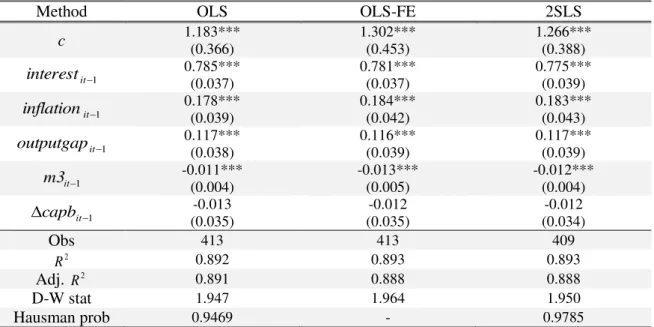
The estimation for central banks’ reaction function is presented in Table 6.
Whilst estimating regression (5), the expected results are ,0 and , 0, and as the three methods meet these hypotheses, we continue to focus on the 2SLS estimation.8
The two main conclusions from this estimation are: 1) central banks are concerned with price stability and economic growth, and with an intermediate goal regarding monetary aggregates; and, on the other hand, 2) central banks do not appear to
react much to a country’s fiscal stance.
Nevertheless, the results exhibit statistical significance for the estimated coefficients of inflation, output gap and M3: whenever there is a 1% increase in the
previous year’s rate of inflation or output gap, central banks raise the short-term interest rate by 0.183% and 0.117%, respectively; and an increase of 1% of M3 implies a decrease of 0.012% of interest rate to meet the goal. Also, the estimated coefficient for the change in the primary balance is not significant, which means central banks do not respond in this way to fiscal policy.
8
16 Table 6
Estimation of central banks’ reaction function with interestit as dependent variable: 1970-2012
Method OLS OLS-FE 2SLS
c 1.183***
(0.366)
1.302*** (0.453)
1.266*** (0.388)
1
it
interest 0.785***
(0.037)
0.781*** (0.037)
0.775*** (0.039)
1
it
inflation 0.178***
(0.039)
0.184*** (0.042)
0.183*** (0.043)
1
it
outputgap 0.117***
(0.038)
0.116*** (0.039)
0.117*** (0.039)
1
it
m3 -0.011***
(0.004)
-0.013*** (0.005)
-0.012*** (0.004)
1
capbit -0.013
(0.035)
-0.012 (0.035)
-0.012 (0.034)
Obs 413 413 409
2
R 0.892 0.893 0.893
Adj. 2
R 0.891 0.888 0.888
D-W stat 1.947 1.964 1.950
Hausman prob 0.9469 - 0.9785
Notes: *, ** and *** represent statistical significance at 10%, 5% and 1% levels, respectively. The robust standard errors are in brackets. Obs represents the total number of observations. D-W stat is the Durbin-Watson statistic. Hausman prob refers to the probability reached in the Hausman test.
Table 7 displays the results for a SUR estimation regarding to the central bank’s
reaction function of each country. According to Wyplosz (1999), a positive sign for the estimated primary balance coefficient implies a complementary relation between both authorities. However, in all countries, apart from Belgium and Spain, the cyclically-adjusted primary balance is not statistically significant, which is what we already expected, given the panel results: based on the lack of evidence concerning central
banks’ response to fiscal policy.
Comparing these results to the benchmark SUR estimation of monetary policy, in most of these countries, their respective interest rates are influenced by the same, or additional factors, such as Austria, Finland, Greece, Italy, Portugal and the United Kingdom.
17 Table 7
SUR estimation of central banks’ reaction function with interestit as dependent variable: 1970-2012
Countries c interestit1 inflationit1 outputgapit1 m3it1 capbit1 Obs R2
Austria 5.860*** (2.130) 0.633*** (0.110) -0.104 (0.176) 0.308** (0.132) -0.045** (0.022) 0.118
(0.113) 33 0.744
Belgium 3.454*** (1.275) 0.646*** (0.087) 0.122 (0.079) -0.030 (0.115) -0.027** (0.012) -0.276***
(0.093) 39 0.815
Denmark 2.509 (2.493) 0.785*** (0.094) 0.110 (0.120) 0.181 (0.124) -0.028 (0.036) -0.047
(0.164) 41 0.785
Finland 6.236*** (1.802) 0.739*** (0.064) 0.046 (0.086) 0.141** (0.063) -0.091*** (0.031) -0.166
(0.104) 37 0.664
France 2.896*** (1.107) 0.617*** (0.076) 0.004*** (0.075) (0.092) 0.152* -0.028* (0.015) (0.150) 0.081 34 0.546
Germany (1.309) 1.844 0.824*** (0.199) -0.541** (0.253) (0.118) 0.117 (0.010) -0.005 (0.049) 0.034 20 0.286
Greece (2.350) 0.430 0.605*** (0.095) 0.615*** (0.106) (0.145) -0.073 (0.026) -0.018 (0.126) -0.186 24 0.698
Ireland (1.904) 2.366 0.705*** (0.122) (0.137) 0.041 (0.092) 0.121 (0.017) -0.015 (0.042) -0.023 27 0.615
Italy (1.322) 1.302 0.729*** (0.072) 0.225** (0.286) (0.116) 0.158 (0.019) -0.011 (0.108) -0.134 32 0.894
Netherlands 3.175*** (1.048) 0.532*** (0.090) (0.088) 0.050 (0.117) 0.186 (0.009) -0.013 (0.118) 0.182 37 0.606
Portugal (1.629) 1.445 0.619*** (0.064) 0.300*** (0.050) 0.348*** (0.092) (0.016) -0.008 (0.081) 0.060 35 0.382
Spain (0.833) 0.681 0.740*** (0.102) -0.507*** (0.161) 0.356*** (0.079) 0.013** (0.006) 0.374*** (0.082) 17 0.776
Sweden (1.567) -0.236 0.908*** (0.200) (0.322) -0.331 (0.157) 0.161 (0.023) 0.020 (0.171) -0.103 19 0.662
United Kingdom 4.694*** (1.321) 0.478*** (0.164) 0.180 (0.235) 0.371** (0.161) -0.021** (0.009) 0.023
(0.113) 23 0.712 Notes: *, ** and *** represent statistical significance at 10%, 5% and 1% levels, respectively. The robust standard errors are in brackets. Obs represents the total number of observations. SUR linear estimation after one-step weighting matrix; total system with 413 observations.
4.2.2. Reaction Function of the National Governments
For the fiscal reaction function, we follow the same approach as Wyplosz (1999), with regards to the choice of explanatory variables, but without relative unit labour costs. Still, we have decided to introduce the first-differences of the short-term interest rate, in order to attain most of the expected results. Hence, the regression is presented as follow:
. (6)
The estimated results are summarised in Table 8. Naturally, primary balance stills reacts positively to government debt ( 0), and its impact is larger than when we consider the simple fiscal policy reaction function (4). Output gap is also statistically
it it it it it it i
18
significant and the result is the expected one ( 0). In fact, governments are concerned with cyclically conditions: whenever the output gap deteriorates by 1%, the primary balance improves by 0.245%.
Table 8
Estimation of national governments’ reaction function with capbit as dependent
variable: 1970-2012
Method OLS OLS-FE 2SLS
c (0.393) -0.624 -3.236*** (0.708) -3.280*** (0.606)
1
it
capb 0.819***
(0.078)
0.707*** (0.084)
0.702*** (0.068)
1
interestit -0.012
(0.053)
-0.029 (0.051)
-0.143 (0.143)
1
it
inflation 0.014
(0.035)
0.123*** (0.046)
0.134*** (0.039)
1
it
outputgap 0.062
(0.050)
0.199*** (0.060)
0.245** (0.123)
1
it
debt 0.012***
(0.003)
0.047*** (0.008)
0.047*** (0.007)
Obs 423 423 410
2
R 0.680 0.725 0.723
Adj. 2
R 0.676 0.713 0.711
D-W stat 2.029 2.064 2.149
Hausman prob 0.000 - 0.000
Notes: *, ** and *** represent statistical significance at 10%, 5% and 1% levels, respectively. The robust standard errors are in brackets. D-W stat is the Durbin-Watson statistic. Hausman prob refers to the probability reached in the Hausman test.
The significance of inflation is also interesting. Therefore, the fiscal authority must achieve the necessary levels of primary budgetary surpluses, to ensure that its budget constraint is consistent with the price level determined by the monetary authority. The results precisely show a reduction of 0.134% in the cyclically adjusted budget deficit after a 1% increase in inflation. This is the basic process that occurs in a Ricardian fiscal regime.
In all of the methods used to estimate the regression, the interest rate variation is the only variable that is not statistically significant. Yet, the displayed signal is the expected one ( 0), indicating again that there is a substitution relationship between both authorities: whereby increases in interest rate lead to a more relaxed fiscal policy, as mentioned by Wyplosz (1999).
19
measure of fiscal stance. Excluding France and Spain, Table 9 shows that result for all countries, which shows that their governments follow a Ricardian fiscal regime.
Table 9
SUR estimation of national governments’ reaction function with capbit as dependent variable: 1970-2012
Countries c capbit1 Δinterestit1 inflationit1 outputgapit1 debtit1 Obs R2
Austria -2.987** (1.227)
0.101 (0.119)
0.169* (0.092)
0.040 (0.120)
0.430*** (0.115)
0.056***
(0.017) 36 0.504
Belgium -3.368*** (1.244)
0.663*** (0.094)
-0.116 (0.128)
0.023 (0.092)
0.203 (0.174)
0.039***
(0.011) 41 0.828
Denmark -0.909 (0.732)
0.736*** (0.081)
-0.089 (0.094)
0.029 (0.058)
0.172* (0.090)
0.035***
(0.011) 41 0.785
Finland (1.224) -1.822 0.667*** (0.105) (0.150) -0.037 0.313*** (0.088) (0.094) 0.180* 0.054** (0.023) 37 0.664
France (0.719) -0.412 0.652*** (0.127) (0.104) -0.036 (0.057) 0.045 (0.090) -0.096 (0.0113) -0.001 34 0.546
Germany -5.945* (3.327) (0.153) -0.078 (0.400) 0.574 (0.370) 0.415 (0.325) -0.102 0.094** (0.046) 20 0.286
Greece -13.606*** (4.013) 0.667*** (0.094) -0.371** (0.145) 0.319*** (0.089) (0.250) 0.320 0.107*** (0.034) 24 0.698
Ireland -7.022*** (2.495) 0.421*** (0.131) (0.541) 0.102 1.133*** (0.417) (0.390) 0.246 0.061** (0.029) 27 0.615
Italy -16.433*** (3.776) 0.454*** (0.105) (0.144) -0.044 0.286*** (0.099) (0.158) 0.104 0.151*** (0.032) 32 0.894
Netherlands -2.855** (1.133) 0.691*** (0.096) 0.270** (0.118) 0.238** (0.097) -0.251** (0.126) 0.043*** (0.016) 37 0.606
Portugal -5.943*** (1.798) 0.473*** (0.111) (0.156) -0.223 0.126** (0.055) 0.370*** (0.126) 0.073*** (0.024) 35 0.382
Spain -4.187* (2.458) 0.984*** (0.203) (0.402) -0.399 (0.488) 0.399 (0.265) -0.116 (0.039) 0.050 17 0.776
Sweden (1.314) 0.251 0.330** (0.136) (0.199) 0.173 -0.452** (0.210) (0.164) 0.168 0.047** (0.019) 19 0.662
United Kingdom
-5.270*** (1.467)
0.810*** (0.098)
-0.289 (0.237)
-0.002 (0.146)
0.446* (0.253)
0.103***
(0.028) 23 0.712 Notes: *, ** and *** represent statistical significance at 10%, 5% and 1% levels, respectively. The robust standard errors are in brackets. Obs represents the total number of observations. SUR linear estimation after one-step weighting matrix; total system with 423 observations.
20
Comparing this test to the SUR estimation of central banks’ reaction function,
the results lead us to conclude that the relationship between a national government and its central bank does not change in both estimations when the interest rate is statistically significant. For example, the short-term interest rates from Austria and the Netherlands positively influence primary balance, which suggests a complementary relationship;
whilst the negative sign for Greece’s interest rate suggests a substitution relationship. However, if interest rate is not significant, then the relationship between both authorities
could change in the SUR estimations of central banks and national governments’
reaction functions. In the cases of Belgium, Denmark, Finland, Germany and Italy, the relationship does not alter, which is contrary to France, Ireland, Portugal, Spain, Sweden and the United Kingdom.
4.3. Institutional Variables
In this section we once again estimate regressions (3) and (4) with the goal of studying the effects that three institutional events – the Maastricht Treaty, the SGP and the introduction of the Euro – had on the monetary and fiscal policies of our country sample. All of these three variables are included in the previous regressions as dummy variables. Another event is the combination of banking, currency, inflation crises and even stock market crashes,9 which represent the total number of crises each country faced through time.
Table 10 and Table 11 report the estimation results of the effects of these events on monetary policy and fiscal policy, respectively, using the 2SLS method10, with random and fixed effects for the estimations of monetary and fiscal policies, respectively, as induced by the Hausman test.
Regarding monetary policy, the Maastricht Treaty, besides the similar, but smaller effect of the SGP and of the introduction of the Euro, is related to a sharp decline in short-term interest rate of 1.563%. This probably occurred because it was the initial step towards creating a more united Europe, and thus represented the so-called convergence process between all the EU members. Within these three events, the goals of central banks remain statistically significant, being namely the impact that inflation has on monetary policy increased along time. Nevertheless, M3 turned out to gain more
9
The regression of the effect each crisis has individually on both policies is estimated through OLS, OLS-FE and 2SLS methods, and it is present in the Appendix – Additional Estimation Results, Table 16. 10
21
relevance with the introduction of the Euro, as concerns with monetary aggregates reference values became secondary goals for central banks.
Table 10
2SLS estimation of institutional variables’ effect on monetary policy with interestit as dependent variable: 1970-2012
Test (1) (2) (3) (4) (5)
c 2.130*** (0.460) 2.016*** (0.473) 1.430*** (0.403) 1.161*** (0.389) 1.309*** (0.408)
1 it interest 0.758*** (0.035) 0.703*** (0.045) 0.752*** (0.040) 0.791*** (0.033) 0.762*** (0.039) 1 it inflation 0.108*** (0.031) 0.170*** (0.031) 0.175*** (0.032) 0.185*** (0.032) 0.192*** (0.032) 1 it outputgap 0.112*** (0.038) 0.132*** (0.040) 0.115*** (0.039) 0.101*** (0.038) 0.114*** (0.040) 1 it m3 -0.003 (0.004) -0.005 (0.004) -0.008** (0.004) -0.007* (0.004) -0.004 (0.004) it dmt -1.563***
(0.290) - - - -
it
dsgp - -1.306***
(0.310) - - -
it
dez - - -0.645***
(0.222) -
-0.483** (0.222)
1
it
crisis - - - -0.619***
(0.152)
-0.589*** (0.153)
Obs 497 497 497 483 483
2
R 0.887 0.886 0.882 0.880 0.882
Adj. 2
R 0.886 0.881 0.881 0.879 0.880
D-W stat 2.117 1.992 2.046 2.008 1.989
Hausman prob 0.1719 0.4592 0.9548 0.9366 0.8827 Notes: *, ** and *** represent statistical significance at 10%, 5% and 1% levels, respectively. The robust standard errors are in brackets. Obs represents the total number of observations. D-W stat is the Durbin-Watson statistic. Hausman prob refers to the probability reached in the Hausman test.
22
than necessary to achieve a higher primary balance to meet this increase in outstanding government debt. These results are in line with Baskaran (2009), who finds that the
Maastricht treaty’s provisions did not have the expected positive effect on economic growth and fiscal outcomes, especially after the introduction of the Euro. Galí and Perotti (2003) also mention that fiscal policy did not became less countercyclical after the Maastricht treaty.
Table 11
2SLS estimation of institutional variables’ effect on fiscal policy with capbit as dependent variable: 1970-2012
Test (1) (2) (3) (4) (5)
c -1.609*** (0.346) -1.563*** (0.346) -1.585*** (0.347) -1.422*** (0.361) -1.391*** (0.365)
1
it
capb 0.744***
(0.075)
0.744*** (0.075)
0.740*** (0.074)
0.718*** (0.089)
0.737*** (0.093)
1
it
debt 0.036***
(0.006)
0.035*** (0.005)
0.034*** (0.005)
0.030*** (0.006)
0.033*** (0.006)
it
dmt -0.610**
(0.237) - - - -
it
dsgp - -0.681***
(0.223) - - -
it
dez - - -0.817***
(0.237) -
-0.757*** (0.241)
1
it
crisis - - - -0.321**
(0.153)
-0.262* (0.144)
Obs 414 414 414 400 400
2
R 0.704 0.705 0.709 0.704 0.711
Adj. 2
R 0.692 0.694 0.697 0.691 0.698
D-W stat. 2.075 2.077 2.105 1.968 2.048
Hausman prob 0.000 0.000 0.000 0.000 0.000 Notes: *, ** and *** represent statistical significance at 10%, 5% and 1% levels, respectively. The robust standard errors are in brackets. Obs represents the total number of observations. D-W stat is the Durbin-Watson statistic. Hausman prob refers to the probability reached in the Hausman test.
While introducing crisisit1 as a variable, the estimated results exhibit that the
total crises of each country had a negative impact along the period of time considered for both policies. Furthermore, when we carried out the tests to determine which crises influenced most these policies, we concluded that banking, inflation and stock market crises affect fiscal policy, whilst only the latter two affect monetary policy.
23
to be negotiated by the governments of each country, and, without any type of support, some countries from the Euro area could become insolvent. Likewise, the ECB is able to establish stability within the monetary union, as well as being able to respect its foundations.
5. Conclusions
Over the last decades the study of the interactions between monetary policy and fiscal policy has gained more relevance, especially after the creation of the EMU, which led to a more distant, less cooperative, relationship. Thus, our study focused on 14 EU countries, and on the well-known major goals of both policies, which are dependent on certain economic variables, as well as trying to determine what type of interactions have been established.
With regards to monetary policy, inflation is the variable which has influenced most the monetary instrument, in addition to output gap and M3, which is no surprise, as price stability is the primary goal of central banks, as proved by the results from their reaction function regression. In fiscal terms, primary balance followed the expected behaviour, by reacting positively to increases in government debt, and the reaction function for national governments evidenced a major concern for levels of public debt, and it did the same, although less so, for the levels of inflation and output gap. All of these conclusions can be related to Ricardian fiscal regimes.
Certain institutional events that affected the EU, namely the Maastricht Treaty, the SGP and the implementation of the Euro, all have a significant effect on the policies followed by policy makers. However, the impact that they have on each policy differs. The Maastricht Treaty was the most significant event for monetary policy, as it was the first step towards a more united Europe; the introduction of the Euro had the greatest effect on fiscal policy, which was a negative one, leading to a decrease in primary balances. In addition, when faced by various crises over the entire period, these events all had a negative impact on both policies.
24
In the country individual analysis, although the majority of the countries belong to the EMU, i.e. monetary policy is the same, fiscal policy is completely different, which thus leads to a variety of interactions across countries, as well as some other results.
References
Afonso, A. (2003). Fiscal Sustainability: the Unpleasant European Case. FinanzArchiv, 61(1), 19-44.
Afonso, A. (2005). Ricardian Fiscal Regimes in the European Union. Empirica, 35(3), 313-334.
Afonso, A. and Toffano, P. (2013). Fiscal Regimes in the EU. European Central Bank Working Paper No. 1529.
Afxentiou, P. (2000). Convergence, the Maastricht Criteria, and their Benefits. The Brown Journal of World Affairs, 7(1), 245-254.
Aiyagari, S. and Gertler, M. (1985). The Backing of Government Bonds and Monetarism. Journal of Monetary Economics, 16(1), 19-44.
Altavilla, C. (2003). Assessing Monetary Rules Performance across EMU Countries. International Journal of Finance and Economics, 8(2), 131-151.
Baskaran, T. (2009). Did the Maastricht treaty matter for macroeconomic performance? A difference-in-difference investigation. Kyklos by Wiley Blackwell, 62(3), 331-358. Bohn, H. (1998). The behaviour of US public debt and deficits. Quarterly Journal of
Economics, 113(3), 949-963.
Clausen, V. and Hayo, B. (2002). Monetary Policy in the Euro Area – Lessons from the First Years. ZEI, Working Paper No. B09-2002, May.
Cukierman, A. (2013). Monetary Policy and Institutions Before, During and After the Global Financial Crisis. Journal of Financial Stability, 9(3), 373-384.
Favero, C. (2002). How do Monetary and Fiscal Authorities Behave? CEPR,Discussion Paper No. 3426, June.
Galí, J. and Perotti, R. (2003). Fiscal Policy and Monetary Integration in Europe. Economic Policy, 18(37), 533-572.
Gerlach, S. and Schnabel, G. (2000). The Taylor Rule and Interest Rates in the EMU Area. Economics Letters, 67, 165-171.
25
Huchet, M. (2003). Does Single Monetary Policy Have Asymmetric Real Effects in EMU? Journal of Policy Modeling, 25(2), 151-178.
Landolfo, L. (2008). Assessing the Sustainability of Fiscal Policies: Empirical Evidence from the Euro Area and the United States. Journal of Applied Economics, 11(2), 305-326.
Leeper, E. (1991). Equilibria under ‘Active’ and ‘Passive’ Monetary and Fiscal Policies.
Journal of Monetary Economics, 27 (1), 129-147.
Leeper, E. and Davig, T. (2009). Monetary-Fiscal Policy Interactions and Fiscal Stimulus. NBER Working Papers No. 15133, November.
Reinhart, C. and Rogoff, K. (2009). This Time Is Different: Eight Centuries of Financial Folly. Princeton, NJ: Princeton University Press.
Ruth, K. (2007). Interest Rate Reaction Functions for the Euro Area: Evidence from Panel Data Analysis. Empirical Economics, 33(3), 541-569.
Sargent, T. and Wallace, N. (1981). Some Unpleasant Monetarist Arithmetic. Federal Reserve Bank of Minneapolis Quarterly Review, 4(3), 381-399.
Taylor, J. (1993). Discretion versus Policy Rules in Practice. Carnegie Rochester Conference Series on Public Policy, 39, 195-214.
Wooldridge, J. (2009). Introductory Econometrics: a Modern Approach. 4th Ed. Canada: South-Western CENGAGE Learning.
Wyplosz, C. (1999). Economic Policy Coordination in EMU: Strategies and Institutions. In: Deutsch-Französisches Wirtschaftspolitisches Forum (1999). Financial Supervision and Policy Coordination in the EMU, ZEI Working Paper No. B11-1999, January.
26 Appendix
Table 12
OLS estimation of institutional variables’ effect on monetary policy with interestit as dependent variable: 1970-2012
Test (1) (2) (3) (4) (5)
c 1.886*** (0.399) 1.779*** (0.397) 1.393*** (0.354) 1.065*** (0.344) 1.235*** (0.356) 1 it interest 0.757*** (0.031) 0.725*** (0.037) 0.750*** (0.034) 0.788*** (0.029) 0.756*** (0.033) 1 it inflation 0.124*** (0.027) 0.158*** (0.027) 0.168*** (0.028) 0.190*** (0.027) 0.193*** (0.027) 1 it outputgap 0.103*** (0.037) 0.121*** (0.038) 0.113*** (0.038) 0.098*** (0.037) 0.115*** (0.039) 1 it m3 -0.004 (0.003) -0.005 (0.003) -0.006* (0.004) -0.006 (0.004) -0.003 (0.004) it dmt -1.220***
(0.24) - - - -
it
dsgp - -1.098***
(0.243) - - -
it
dez - - -0.777***
(0.196) -
-0.646*** (0.192)
1
it
crisis - - - -0.606***
(0.143)
-0.566*** (0.142)
Obs 513 513 513 499 499
2
R 0.887 0.884 0.882 0.880 0.882
Adj. 2
R 0.886 0.883 0.881 0.879 0.881
D-W stat 2.099 2.033 2.025 2.009 1.981
27 Table 13
OLS estimation of institutional variables’ effect on fiscal policy with capbit as dependent variable: 1970-2012
Test (1) (2) (3) (4) (5)
c -0.406*
(0.215)
-0.363* (0.217)
-0.398* (0.217)
-0.307 (0.239)
-0.224 (0.232)
1
it
capb 0.823***
(0.075)
0.824*** (0.076)
0.815*** (0.074)
0.818*** (0.077)
0.812*** (0.077)
1
it
debt 0.012***
(0.003)
0.012*** (0.003)
0.013*** (0.003)
0.010*** (0.003)
0.012*** (0.003)
it
dmt -0.247
(0.19) - - - -
it
dsgp - -0.378**
(0.191) - - -
it
dez - - -0.625***
(0.200) -
-0.626*** (0.209)
1
it
crisis - - - -0.326**
(0.15)
-0.293** (0.140)
Obs 428 428 428 414 414
2
R 0.679 0.681 0.686 0.680 0.687
Adj. 2
R 0.677 0.679 0.683 0.678 0.684
D-W stat 2.044 2.053 2.066 1.971 2.003
28 Table 14
OLS-FE estimation of institutional variables’ effect on monetary policy with interestit
as dependent variable: 1970-2012
Test (1) (2) (3) (4) (5)
c 2.280*** (0.484) 1.984*** (0.463) 1.476*** (0.422) 0.941** (0.419) 1.087*** (0.426) 1 it interest 0.738*** (0.032) 0.697*** (0.038) 0.737*** (0.034) 0.783*** (0.029) 0.741*** (0.034) 1 it inflation 0.111*** (0.029) 0.158*** (0.029) 0.165*** (0.029) 0.201*** (0.028) 0.199*** (0.028) 1 it outputgap 0.106*** (0.037) 0.134*** (0.040) 0.120*** (0.039) 0.102*** (0.038) 0.127*** (0.040) 1 it m3 -0.005 (0.004) -0.003 (0.004) -0.005 (0.005) -0.004 (0.005) -0.003 (0.004) it dmt -1.467***
(0.250) - - - -
it
dsgp - -1.384***
(0.267) - - -
it
dez - - -0.997***
(0.244) -
-0.970*** (0.241)
1
it
crisis - - - -0.647***
(0.146)
-0.607*** (0.145)
Obs 513 513 513 499 499
2
R 0.888 0.885 0.883 0.881 0.882
Adj. 2
R 0.884 0.881 0.878 0.876 0.881
D-W stat 2.082 2.012 2.008 2.015 1.981
Hausman prob - - - - -
29 Table 15
OLS-FE estimation of institutional variables’ effect on fiscal policy with capbit as dependent variable: 1970-2012
Test (1) (2) (3) (4) (5)
c -1.429***
(0.311)
-1.382*** (0.313)
-1.416*** (0.312)
-1.297*** (0.337)
-1.282 (0.343)
1
it
capb 0.745***
(0.090)
0.746*** (0.092)
0.738*** (0.090)
0.732*** (0.096)
0.733*** (0.097)
1
it
debt 0.032***
(0.005)
0.030*** (0.005)
0.031*** (0.005)
0.028*** (0.006)
0.031*** (0.006)
it
dmt -0.493**
(0.198) - - - -
it
dsgp - -0.511**
(0.206) - - -
it
dez - - -0.717***
(0.218) -
-0.682*** (0.227)
1
it
crisis - - - -0.306**
(0.155)
-0.258** (0.147)
Obs 428 428 428 414 414
2
R 0.707 0.708 0.711 0.706 0.687
Adj. 2
R 0.695 0.697 0.700 0.694 0.684
D-W stat 2.041 2.048 2.061 1.953 2.003
Hausman prob - - - - -
30 Table 16
Estimation of the effects of different types of crises (dummy variables) on monetary and fiscal policies: 1970-2012
Policy Monetary Policy Fiscal Policy
Dependent
Variable interestit capbit
Method OLS OLS-FE 2SLS OLS OLS-FE 2SLS
c 1.053*** (0.377) 1.169** (0.462) 1.071** (0.437) -0.520** (0.245) -1.519*** (0.345) -1.635*** (0.366)
1
it
interest 0.799*** (0.029) 0.795*** (0.028) 0.799*** (0.037) - - -
1
it
inflation 0.125*** (0.025) 0.127*** (0.028) 0.130*** (0.034) - - -
1
it
outputgap (0.045) 0.013 (0.046) 0.009 (0.046) 0.017 - - -
1 it m3 -0.010** (0.004) -0.012** (0.006) -0.011**
(0.005) - - -
1
it
capb - - - 0.906***
(0.052) 0.817*** (0.083) 0.785*** (0.095) 1 it
debt - - - 0.010***
(0.003) 0.027*** (0.006) 0.029*** (0.006) it dbc -0.279 (0.264) -0.277 (0.277) -0.333 (0.276) -1.119*** (0.361) -1.288*** (0.325) -1.372*** (0.324) it dcc -0.036 (0.294) 0.009 (0.302) -0.074 (0.297) 0.206 (0.328) 0.371 (0.349) 0.358 (0.355) it dic 2.172** (1.035) 2.230** (1.049) 2.090** (1.055) 1.106* (0.597) 1.393** (0.629) 1.238* (0.640) it dsmc 0.920*** (0.212) 0.955*** (0.215) 0.974*** (0.220) 0.235 (0.216) 0.431** (0.204) 0.480** (0.205)
Obs 483 483 467 398 398 384
2
R 0.878 0.879 0.878 0.725 0.745 0.744
Adj. 2
R 0.876 0.873 0.876 0.721 0.733 0.730
D-W stat 1.963 1.965 1.974 1.756 1.740 1.716
Hausman prob 0.9196 - 0.9514 0.0007 - 0.0084