Estimating wildlife mortality at wind farms: accouting for carcass removal, imperfect detection and partial coverage

(1)

Universidade de Lisboa

Faculdade de Ciˆencias

Departamento de Estat´ıstica e Investiga¸c˜

ao Operacional

Estimating wildlife mortality at wind farms: accounting

for carcass removal, imperfect detection and partial

coverage

Regina Maria Baltazar Bispo

Tese orientada pelos Professor Doutor Dinis Pestana e Doutor Tiago A.

Marques especialmente elaborada para obten¸c˜ao do grau de doutor em

Estat´ıstica e Investiga¸c˜ao Operacional (Especialidade em Estat´ıstica

Experimental e An´alise de Dados)

(2)

(3)

Acknowledgements

This thesis would not have been possible without the support of several people. Professor Dinis Pestana was the ﬁrst to make it possible. He made me believe that I could begin and ﬁnish this journey. During these years I have learn with him many things within and largely beyond the statistics domain. It was a privilege for me to work with him. Thank you, Dinis.

Doctor Tiago A. Marques was a perfect supervisor. Young enough to be completely available and old enough to push me to another scientiﬁc level. I have learn so much with him that is almost impossible to put it in words. Thank you for pushing me the way you did, for all the discussions and for the exhaustive text revisions.

I’m also thankful to BIO3–Estudos e Projectos em Biologia e

Val-oriza¸c˜ao de Recursos Naturais which provided the motive to this

the-sis. They allowed me to use their data and partially sponsored my work. The executive managers Hugo Costa and Miguel Mascaren-has were always available and cooperative. A special word for Joana

(4)

ii

Bernardino that always reminded me of the ecological importance of the work. The discussions with her were really important and helpful.

To ISPA–Instituto Universitário, for partially supporting the edition of this thesis. The Centro de Estat´ıstica e Aplica¸cões da Universidade de Lisboa provided some financial support to participate in conferences

through the Funda¸c˜ao Nacional para a Ciˆencia e Tecnologia, Portugal

- FCT under the project PEst-OE/MAT/UI0006/2011.

From all the people that made a diﬀerence, Jo˜ao Nuno was certainly

one of them. Because the next words are for him, I will write them in

Portuguese. Durante todo o caminho foi bom ter algu´em ao lado que

me dava a calma e a seguran¸ca que eu precisava para continuar. Porque quando eu duvidava, tu me fazias acreditar e porque nos melhores e

(5)

Resumo

A produ¸cão de energia eólica, à semelhan¸ca de outras energias

renov´aveis, apresenta diversas vantagens relativamente `as fontes de

energia tradicionais. Contudo, hoje em dia, ´e reconhecida a existˆencia

de potenciais impactes, nomeadamente sobre os sistemas biol´ogicos.

Entre os grupos faun´ısticos mais afectados encontram-se os

vertebra-dos voadores, podendo a constru¸c˜ao destes projectos ser respons´avel,

por exemplo, pela perda directa e altera¸c˜ao de habitat, efeito de

bar-reira ou perturba¸cão das áreas de nidifica¸cão. Embora nos últimos

anos tenha sido dada aten¸c˜ao aos v´arios impactes, a mortalidade de

aves e quir´opteros, directamente causada pela colis˜ao com os

aeroger-adores tem sido o impacte que maior preocupa¸c˜ao desperta. Uma

questão central na monitoriza¸cão de parques eólicos prende-se, por

isso, com a quantifica¸cão da mortalidade de aves e quirópteros

cau-sada por colis˜ao com os aerogeradores. Nos estudos de monitoriza¸c˜ao

a estima¸c˜ao da mortalidade baseia-se na contagem de animais

mor-tos. Por´em ´e amplamente reconhecido que a mortalidade observada

subestima a mortalidade real. As principais raz˜oes que justiﬁcam esta

(6)

iv

diferen¸ca prendem-se com (1) a ocorrência de remo¸cão de cadáveres

de aves/morcegos (por predadores, decomposi¸c˜ao ou outro), (2) a

de-teçcão imperfeita pelos observadores e (3) a prospeçcão parcial do

par-que. Conceptualmente, a quantiﬁca¸c˜ao da mortalidade tem por base

a ideia de que a mortalidade real poder´a ser estimada corrigindo a

mortalidade observada com a probabilidade de encontrar um cad´aver.

A diferen¸ca entre as mortalidades real e observada ser´a tanto maior

quanto menor for esta probabilidade. Assumindo que os cad´averes s˜ao

encontrados independentemente uns dos outros, ent˜ao o n´umero de

cadáveres encontrados numa visita ao parque é uma variável aleatória

binomial com parâmetros definidos pelo número de animais mortos na

regi˜ao de estudo (dimens˜ao da popula¸c˜ao, N ) e probabilidade de

en-contrar um cad´aver (P ). Nestas condi¸c˜oes, assumindo a probabilidade

de encontrar um cad´aver conhecida, o estimador de m´axima

verosim-ilhan¸ca do n´umero de animais mortos presentes na regi˜ao no dia da

visita é dado pela razão entre o número de cadáveres encontrados e

a probabilidade de encontrar um cad´aver. Contudo, na maiorias das

situa¸c˜oes, esta probabilidade ´e desconhecida. Assim, estimar N

im-plica estimar P . Para encontrar um cad´aver em campo ´e necess´ario

que ele (1) esteja na ´area prospectada (´area coberta na amostragem

deﬁnida por desenho experimental), (2) esteja dispon´ıvel para ser en-contrado e (3) seja detectado pelo observador. Assumindo a

inde-pendˆencia entre os trˆes acontecimentos, a probabilidade de encontrar

um cadáver é dada pelo produto entre a probabilidade de inclusão

da ´area prospectada na amostra, a probabilidade de estar dispon´ıvel

(7)

v

prospectada e a probabilidade de deteçcão do cadáver dado que se

encontra na ´area prospectada e n˜ao foi removido.

Tipicamente num estudo de monitoriza¸c˜ao de um parque e´olico, o

campo ´e dividido em tantas ´areas quantos turbinas existirem, sendo

selecionadas por amostragem aleat´oria simples as turbinas a incluir

no estudo, cuja área de influencia será prospectada. Assim, a

proba-bilidade de inclusão desta área no processo de amostragem é definida

por desenho experimental tendo em conta a propor¸c˜ao de turbinas

incluidas no estudo ou a ´area sob inﬂuencia das turbinas selecionadas.

A probabilidade de estar dispon´ıvel para ser encontrado ´e deﬁnida

pela esperan¸ca matem´atica da probabilidade de permanˆencia de um

cadáver. A análise de sobrevivência é uma metodologia estat´ıstica

que possibilita a an´alise de dados relativos a tempos de “vida”, num

sentido lato, isto ´e, que se aplica a todas as situa¸c˜oes em que

inter-essa modelar o tempo até à ocorrência de um determinado

aconteci-mento, aplicando-se por isso, neste dom´ınio. At´e `a presente data, esta metodologia, apesar de adequada ao estudo formal dos tempos de

per-manˆencia, n˜ao tem sido utilizada neste contexto. Os estudos

publica-dos são escassos e as metodologias usadas não estão uniformizadas. A análise estat´ıstica dos tempos de remo¸cão é frequentemente limitada a

procedimentos descritivos ou, usando procedimentos inferenciais, n˜ao

tem em conta a t´ıpica assimetria positiva da densidade dos tempos

de permanˆencia e/ou facto de existirem observa¸c˜oes censuradas.

Al-guns autores reconhecem a existˆencia de observa¸c˜oes censuradas,

(8)

vi

a priori uma distribui¸c˜ao exponencial dos tempos de permanˆencia.

A determina¸c˜ao da esperan¸ca matem´atica da probabilidade de

per-manência envolve a estima¸cão da fun¸cão de sobrevivência do tempo

de permanência. As op¸cões de modela¸cão desta variável incluem

metodologias não-paramétricas, semi-paramétricas e paramétricas. A

modela¸cão paramétrica de tempos de permanência, sob validade de

um certo modelo probabil´ıstico, pode permitir obter inferˆencias mais

precisas do que as obtidas por métodos não paramétricos, assumindo

verdadeiro aquele pressuposto. Um dos aspectos fundamentais na

modela¸cão paramétrica é por isso a escolha do modelo probabil´ıstico

subjacente aos dados. O primeiro passo na an´alise do tempo de

per-manência dos cadáveres deverá consistir na explora¸cão da respectiva forma da distribui¸cão. São vários os modelos paramétricos

repetida-mente encontrados na literatura no ˆambito da modela¸c˜ao de tempos

de “vida”. De entre os mais comuns, tˆem-se os modelos exponencial,

Weibull, log-normal e log-log´ıstico. Os m´etodos dispon´ıveis para a

es-colha de uma distribui¸c˜ao particular incluem al´em de procedimentos

gr´aﬁcos, procedimentos inferenciais que, de um modo mais formal,

val-idam um modelo param´etrico em detrimento de outro. Como ponto

de partida para uma análise de sobrevivência paramétrica rigorosa,

neste estudo são discutidos os métodos de discrimina¸cão entre

mode-los probabil´ısticos para os tempos de permanˆencia registados em testes

de remo¸c˜ao levados a cabo em parques e´olicos nacionais.

A valida¸c˜ao formal de um modelo probabilistico envolve

(9)

dis-vii tribui¸c˜ao emp´ırica. Contudo, no caso de observa¸c˜oes censuradas pouco ´

e conhecido sobre a potˆencia deste tipo de testes. Neste trabalho, foi

feito um estudo por simula¸c˜ao da potˆencia relativa dos testes de

ajusta-mento baseados nas estat´ısticas de Kolmogorov-Smirnov, Cram´

er-Von-Mises e Anderson-Darling, variando as distribui¸c˜oes sob as hip´oteses

nula e alternativa, a dimens˜ao da amostra, o grau de censura e o n´ıvel

de signiﬁcˆancia.

Nesta tese foi tamb´em efectuada a compara¸c˜ao das metodologias

paramétricas e semi-paramétricas (Regressão de Cox) na modela¸cão

da fun¸cão de sobrevivência dos tempos de permanência.

Adicional-mente discute-se a importância da seleçcão do modelo probabilistico

no contexto da estima¸cão da fun¸cão de sobrevivência e mortalidade.

A estima¸cão da probabilidade de deteçcão do cadáver é enquadrada

no contexto formal da amostragem por distˆancias. Neste contexto,

a varia¸cão da detectabilidade é explicada como fun¸cão da distância

entre o objeto e o ponto de amostragem. Na abordagem

conven-cional assume-se que a distribui¸c˜ao dos objetos em rela¸c˜ao aos

pon-tos de amostragem (ponpon-tos ou linhas) ´e uniforme. A utiliza¸c˜ao das

turbinas como pontos a partir das quais ´e efectuada a amostragem dos

cad´averes p˜oe em causa este pressuposto. De facto, dado que a morte

das aves/morcegos ocorre por colisão com as turbinas, a localiza¸cão dos cadáveres está altamente dependente da localiza¸cão das turbinas. Em consequência, a distribui¸cão espacial de cadáveres à volta das turbinas não é uniforme. Neste estudo, considerou-se a utiliza¸cão de uma

(10)

viii

cadáveres em torno das turbinas. Contudo para responder à não

ver-iﬁca¸c˜ao do pressuposto de uma densidade constante, consideraram-se

as distribui¸cões gama e log-normal para modelar a distribui¸cão espa-cial dos cadáveres.

Conclui-se com a apresenta¸c˜ao de um estimador da mortalidade que

integra no espa¸co e no tempo a mortalidade observada corrigida pela

remo¸c˜ao, detectabilidade imperfeira e cobertura parcial. O estimador

apresentado soluciona algumas das limita¸c˜oes de m´etodos

anterior-mente usados, como sejam, a imposi¸c˜ao da utiliza¸c˜ao de intervalos de

tempo regulares entre amostragens e o pressutosto de uma distribui¸c˜ao

exponencial dos tempos de permanência dos cadáveres até à remo¸cão.

O metodo possibilita ainda a modela¸cão de popula¸cões heterogéneas

e permite considerar densidades n˜ao uniformes de cad´averes em torno

das turbinas.

Palavras-chave: An´alise de sobrevivˆencia, amostragem por

(11)

Abstract

In wind farms, the observed fatality is known to underestimate the real fatality because of carcass removal, imperfect detection and partial coverage.

The maximum likelihood estimator for the number of carcasses is de-ﬁned by the ratio between the number of found carcasses and the encounter probability. Under an independence assumption, this prob-ability can be estimated by the product of (1) the probprob-ability that a carcass is in the covered region, (2) the probability of persisting and (3) the probability of detection. The probability that a carcass is in the covered region is deﬁned by design. The latter probabilities are model-based estimated.

The average probability of persisting is estimated using survival analy-sis. Parametric models based on the exponential, Weibull, log-logistic and log-normal distributions were used as these are among the most common used lifetime models. In this study we explore how to dis-criminate between these four competing models. A common way to

(12)

x

formally test for a distributional assumption is the use of goodness-of-ﬁt (GoF) statistics based on the empirical distribution function. The statistical power of some GoF statistics was investigated varying the null and the alternative distributions, the sample size, the degree of censoring and the signiﬁcance level. The results obtained from using semiparametric and parametric methods to model data collected at ten Portuguese wind farms are presented and compared.

The average detection probability is deﬁned using distance sampling approach, considering point transect at turbines locations. Conven-tional distance sampling assumes a constant mean density with re-spect to samplers’ location. In wind farms the spatial distribution of the dead animals is known to be highly dependent on the turbine lo-cation. Hence, non-uniform density around sampling points has been considered.

This study concludes presenting a mortality estimator that integrates over space and time the observed fatality corrected for carcass removal, imperfect detection and partial coverage.

Keywords: Distance sampling, mortality estimation, parametric

(13)

Chapter 1 Introduction

1.1 The non-statistical framework

The human inﬂuence on the environment is today a consensual mat-ter of concern. For decades humans used the natural resources with little concern for the negative consequences on the environment. That lead to many situations of clear degradation of the natural resources. Today, the consequences on biodiversity are well known. Threats are directly linked to the loss of habitats due to destruction, modiﬁcation and fragmentation of ecosystems and direct mortality.

As a consequence of the growing awareness of the possible negative impacts on nature resulting from human activities, in many coun-tries there is speciﬁc legislation that governs the decisions about

(18)

4 _Introduction plementing and developing projects that are likely to have negative environmental impacts. In this context, the Environmental Impact Assessment (EIA) emerges as a tool by which information about the environmental eﬀects of a project is collected, impacts are predicted and mitigation measures are identiﬁed (Wale and Yalew, 2010).

The EIA includes a pre-construction evaluation phase and a

post-construction monitoring phase. In the pre-construction phase the

risk to wildlife is evaluated and the data collected are used to de-sign the project aiming to avoid or minimize the environmental risks. At the end of pre-construction studies, decisions are made regarding the project implementation that may result in implement, delay or even abandon the project in favor of sites with less potential for en-vironmental impact and other sites or landscapes may be evaluated in search of more acceptable sites for development. Most likely, the final decisions focus on how to develop a project and avoid, minimize or mitigate the potential effects that have been identified during the pre-construction study (Strickland et al., 2011).

The post-construction phase includes monitoring the impacts posed by the speciﬁc projects during construction and exploration. In this phase the main goal is to evaluate the impacts, if necessary to adopt new measures to overcome unpredicted or under-evaluated risks and to check the usefulness of the mitigation measures previously proposed. It is during this phase that the actual impacts on animal species are deﬁned. In particular, the evaluation of the mortality caused by the human-made structures is a key issue in post-construction studies.

(19)

Introduction 5 In the literature it is easy to find references to mortality numbers linked to obstacles such as vehicles, aircrafts, buildings, windows, power lines and communication towers (Jana and Pogacnik, 2008). Currently, fa-tality of flying vertebrates through collision with rotating turbine rotor blades and other structures in wind farms receives great attention as consequence of the growing risk posed by the rapid increase in the number of wind turbines worldwide (Drewitt and Langston, 2008). In the wind farm projects, post-construction fatality studies, beside helping in characterizing the species composition of fatalities and in identifying the factors related to higher mortality, focus primarily on estimating the fatality rate for birds and bats and in many cases the total estimated fatalities at an operating wind energy facility (Strick-land et al., 2011). Information regarding mortality is crucial in several contexts, namely, to understand how pre-construction registered ac-tivity at a site is related to post-construction mortality, to compare mortality between sites or under several conditions and/or to evaluate the efficiency of mitigation (Huso, 2010).

Behind this ecological problem lies a statistical problem. In the next section, I will deﬁne this statistical problem aiming to respond to the basic, general and yet hard to answer question “How many fatalities?”.

(20)

6 _Introduction

1.2 The statistical problem

Nowadays, the estimation of mortality is mandatory in every human project with a direct impact on wildlife. The problem of estimating mortality is therefore an issue on a broad diversity of situations. Here I will focus only on the problem of estimating the mortality in wind farms, although this problem is not at all restricted to this type of projects.

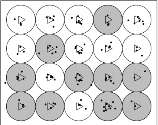
Consider a wind farm where turbines are regularly spaced on an homo-geneous terrain. Under these conditions by assuming complete avail-ability and perfect detection, the true number of dead animals could be simply estimated just dividing the number of observed carcasses by the proportion of the searched area. Figure 1.1 illustrates the result of a search in a wind farm with 20 turbines. As half of the turbines were searched, if we assume that all the carcasses within the searched area were detected, then 96 birds are estimated to have died in the ﬁeld.

In practice, however, one never knows the proportion of the population that was available to be detected neither the proportion of the pop-ulation that was detected. In general, mortality assessment is based on correcting the number of bird carcasses found in the wind farms (observed mortality) for several sources of uncertainty. One of these sources of uncertainty that is directly related to the availability for detection is the removal of dead bird carcasses by, e.g., scavengers, predators or decomposition. To account for carcass removal, we need

(21)

Introduction 7

Figure 1.1: Detected carcasses (dots) found by searching the shaded areas (randomly selected turbines), which represents half of the wind farm turbines

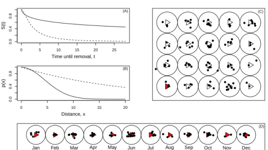
to estimate the probability of persistence of a carcass. Hence, mod-eling time until carcass removal is a key part of estimating mortality. The time of removal will depend on factors such as the animal char-acteristics (e.g., size) and the environmental conditions (e.g. season). Hence, these variables should be considered when estimating the prob-ability of persistence of a carcass as removal rate will diﬀer depending on these (and other) conditions. Figure 1.2 (A) shows two persistence curves illustrating two diﬀerent carcass removal rates.

In most real situations, we are not able to detect all the carcasses in the searched area. So, the other key factor in this process is the observers ability to detect the carcasses and the estimation of the prob-ability of detection. Additionally, while estimating this probprob-ability it is also important to consider its dependency on factors such as the animal characteristics, the environmental conditions and the observer

(22)

8 _Introduction

0 5 10 15 20 25

0.0

0.4

0.8

Time until removal, t

S(t) (A) 0 5 10 15 20 0.0 0.4 0.8 Distance, x p(x) (B) (C)

Jan Feb Mar Apr May Jun Jul Aug Sep Oct Nov Dec

(D)

Figure 1.2: Estimating mortality in wind farms. (A) Probability of carcass persisting (S(t)) as a function of time until removal (t). The plot illustrates two diﬀerent removal rates (solid line - slower removal and dashed line - faster removal), (B) Probability of detection (p(x)) as a function of the distance between the carcass and the observation point (x). The plot of illustrates two decreasing rates of detectability with distance (solid line - faster decreasing detectability and dashed line - slower decreasing detectability), (C) Spatial variation of mortal-ity, (D) Temporal variation of mortality

(23)

Introduction 9 characteristics. Figure 1.2(B) illustrates the concept showing the vari-ation of the detection searcher ability with animals distance from the observation point for two diﬀerent decreasing rates.

Also, there is spacial (Figure 1.2(C)) and temporal variability (Figure 1.2(D)) associated with this process. In wind farms the terrain is typically non homogeneous having several types of covering vegetation and a more or less complex orography. This spatial variability imposes diﬀerent exposures to dead animals which inﬂuences carcass removal and detection. Additionally, because mortality is collision-based, the distribution of the dead animals is associated with the turbine location. Hence, the expected carcass density in the “fall zone” will vary and typically decrease with the distance to the turbine.

When estimating the mortality in this type of projects it is common to aim for an annual estimate. Hence, mortality must be integrated not only over space but also over time.

To illustrate the mortality estimation problem let us consider a site with 12 turbines in which 2 animals die per day per turbine, i.e., a daily total of 24 dead animals over the entire wind farm. Assuming that from the 24 animals that die in each day (persistence probability of 1), 12 will persist to the next day (persistence probability of 0.5) and that none persist beyond that (persistence probability of 0), a total of 36 dead animals will be present in each day, 12 that persisted from the previous day and 24 that died at that day and the persistence expectancy is 1.5. Assuming a perfect detection and that 50% (6 out

(24)

10 _Introduction of the 12 turbines) of the survey area was covered by the design, we would see 18 dead animals, yielding a mortality corrected for partial coverage of 18/0.5 = 36. Dividing this number by the persistence

expectancy yields a mortality of 36/1.5 = 24 animals. Hence, _0.518_×1.5

estimated the true mortality at the visit day. Considering this day as representative of a time interval of, say, 4 days, then the estimated mortality for this time period would be given by _0.518_×1.5×4 .

In summary, my goal is to estimate the mortality over a period of time for a speciﬁc region (region under the inﬂuence of the wind farm), based on the information that we get from multiple time surveys over a fraction of this region (covered region). If, at a particular survey, n carcasses were observed then, as the previous example stresses, to estimate the true mortality this value has to be scaled up by the pro-portion of the covered area and adjusted for persistence. If additionally we considered that detection is not perfect, then this component has also to be considered.

1.3 Research goals and thesis outline

This research aims at providing support for monitoring studies on wildlife fatalities and establishing a methodology to estimate mortality at a wind farm. To do that I have reviewed the current methods and analyzed the available estimators. Ultimately, I propose alternative analytical approaches to estimate mortality.

(25)

Introduction 11 This thesis is organized in ﬁve more chapters of which a brief outline is given below:

Chapter 2 presents a summary of the currently used methods to

es-timate the wildlife fatality either published in peer-reviewed lit-erature or used in practice, even if not published.

Chapter 3 presents the maximum likelihood estimation method as a

statistical rationale to formally deﬁne a mortality estimator. The state and observation models conceptual framework is deﬁned in this context.

Chapter 4 addresses the problem of estimating the average

probabil-ity of carcass persisting and modeling time until carcass removal as a key factor to estimate wildlife mortality. Three papers were published addressing this topic.

The ﬁrst paper (section 4.1) focuses on (1) proposing a method-ological strategy to discriminate between several plausible para-metric survival models suitable for modeling the removal times of carcasses and (2) exemplifying the proposed methodology using data collected in trials conducted at Portuguese wind farms. The second paper (section 4.2) establishes a complete statisti-cal methodology for analyzing data from removal trials and es-timating the average probability of carcass persistence. Using data sets collected at ten Portuguese wind farms we compared diﬀerent survival analysis strategies (semiparametric and para-metric) that can be used to model carcass removal time data.

(26)

12 _Introduction We investigated the impact that different modeling assumptions can have on estimated mortality rates. Ultimately, we aimed at establishing a reliable statistical methodology for analyzing data from removal trials that avoids reporting findings exclusively on the grounds of empirical estimates promoting instead the use of adequate statistical models as a consequence of proper compar-ative goodness-of-fit analysis regarding diverse plausible models. Goodness-of-fit (GoF) tests are a formal procedure to test the significance of the discrepancy between an empirical distribution function and an assumed true distribution function. Although this type of procedures is widely used in research, investigations about the power of GoF statistics for censored data are scarce. In the third paper (section 4.3) the power of common GoF statistics is investigated varying the null and the alternative distributions (completely specified), the sample size, the significance level and the degree of censoring.

Chapter 5 describes the estimation of the detection probability

based on the distance sampling conceptual framework. The av-erage detection probability estimation is reviewed considering point transect at turbines locations, assuming both uniform and non-uniform densities of carcasses around the sampling points.

Chapter 6 provides a conclusion on the results of the study and

(27)

Chapter 2 Current conceptual model

for mortality estimation

Current approaches used to estimate wildlife mortality are based on the idea that the true mortality can be obtained adjusting the num-ber of observed carcasses for carcass removal and searchers’ detection ability. Here I list the most commonly used and recently developed mortality estimators:

1. Erickson et al. (2001) deﬁne the mortality estimator dividing the number of found carcasses (n) by the product between the probability that a carcass is detected by the observer (p) and the

mean time of removal (¯t). Considering a time interval of length

I between searches, the estimator is deﬁned by the authors as 13

(28)

14 _{Current conceptual model} ˆ N = n (¯tp)/I (2.1) where ¯t = ∑c i=1ti

c−c′ , with c and c′ representing the total number

of carcasses placed in a removal carcass trial and the number of carcasses for which time of removal was right censored, respec-tively. Implicitly, these authors assume that the removal times

follow an exponential distribution. Note that ¯t is the maximum

likelihood estimator for the mean time of removal assuming an

exponential model with c′ right-censored observations.

2. Shoenfeld (2004) published a report developing two estimators. The ﬁrst estimator is based on the Poisson model. In this ap-proach this author assumes that the number of deaths occur as a Poisson process with rate λ (and, hence, mean time between deaths 1/λ). The number of removed carcasses and the num-ber of searches for carcasses are also assumed to follow a Poisson

model with rate 1/¯t (where ¯t is the mean time between removals)

and 1/I (with I being the mean time between searches), respec-tively. In each search the probability of a carcass being detected by an observer is assumed to be p (carcasses are assumed to be found independently). It is also assumed that no animals die before time zero (before the ﬁrst search).

Assume D(t) to be the expected number of birds killed in the time interval [0, t], G(t) the expected number of birds on the ground (neither removed nor detected) at time t, F (t) the expected number of birds detected in [0, t] and R(t) the

(29)

ex-Current conceptual model 15 pected number of birds removed in [0, t], such as the expected

value of D(t) = λt and G(t) = D(t) − F (t) − R(t). Hence,

D′(t) = λ ⇔ G′(t) + F′(t) + R′(t) = λ. Considering the time

derivatives F′(t) = G(t)(p/I) and R′(t) = G(t)(1/¯t), we get

G′(t) + [(p/I) + (1/¯t)]G(t) = λ or G′(t) + aG(t) = λ, with

a = (p/I) + (1/¯t). Multiplying each term by eat and integrating gives eatG′(t) + aeatG(t) = λeat ⇔ [ eatG(t) ]_′ = λeat ⇔ ∫ t 0 [ eatG(t) ]′ dt = ∫ t 0 λeatdt ⇔ eat_{G(t) =} λ a ( eat ]t 0 ⇔ eat_{G(t) =} λ a ( eat− 1 ) ⇔ G(t) = λ a ( 1− e−at ) .

To deﬁne asymptotically a steady state, let t → ∞. Hence,

G(∞) = λ/a (as (1 − e−at) → 1) and F′(∞) = G(∞)(p/I) = (¯tpλ)/(¯tp + I). Considering a steady state interval of length T , the expected number of birds killed in the interval (N ) and the expected number of birds found in the interval (n) are given by N = λT and n = F′(∞)T , respectively. Hence, N_λ = _F_′₍n_∞) ⇔ N = n(¯tp + I)/(¯tp). Finally,

ˆ

N = n

(30)

16 _{Current conceptual model} The second estimator is deﬁned, assuming periodic searches, reg-ular time intervals between visits and absolute knowledge of re-moval rate and searchers’ detection probability

ˆ N = n ¯ tp I [ exp(I/¯t)−1 exp(I/¯t)−1+p ]. (2.3)

In this case no clear theoretical background is given and, despite the eﬀort, it was not possible to derive this expression.

3. Kerns et al. (2005) present the following deﬁnition for a mortality estimator ˆ N = n 1 I ∑I t=1[1− P (T ≤ t)]p(1 − p)t−1 . (2.4)

Here, the carcass persistence is estimated by the empiric cumu-lative probability distribution function represented by the term 1−P (T ≤ t) that corresponds to the observed probability that a carcass persists at least t days prior to removal. The expression

p(1− p)t−1 is the probability mass function of a geometric

vari-able. Hence, it represents the probability of taking t days until the ﬁrst carcass is detected. Note that although this term aims to account for imperfect detection it is far from representing the average detection probability needed to correct the number of observed carcasses for detectability.

4. Jain et al. (2007) deﬁne the mortality estimator simply by ˆ

N = n

ppr

(31)

Current conceptual model 17 where pris the probability of persisting defined empirically as the proportion of unremoved carcasses after approximately half the actual search cycle, based on the assumption that the probability of a collision event is equally distributed over all days between searches. The probability of detecting a carcass (p), also defined empirically, is estimated by the proportion of carcasses detected by the observers in a search efficiency trial.

5. Huso (2010) recently developed the estimator

ˆ

N = n

pprν

(2.6) where the probability of being detected (p) is estimated based

on trials by ˆp = number observed/number available. The

ad-justment for carcass removal is based on the exponential model for persistence time and the correction factor regarding removal (pr) is generally deﬁned by

pr= ∫I

y=0exp(−y/¯t)dy

I =

¯

t(1− exp(−I/¯t))

I .

Based on the argument that when the interval between searches

greatly exceeds the expected persistence time of a carcass, pr

is biased low inﬂating fatality (because when I increases, pr

decrease), this author deﬁnes the parameter ν, called eﬀective search interval, estimated by ˆν = min(1, ˜I/I), with ˜I represent-ing the length of time beyond which the probability of a carcass

persisting is ≤ 1%, i.e., P (T > ˜I) ≤ 0.01. Assuming an

(32)

18 _{Current conceptual model} e−˜I/¯t _{≤ 0.01 and, thus, the minimum ˜I that satisﬁes this}

condi-tion is ˜I =− log(0.01)¯t. Based on this development the

estima-tor for the average probability of persisting (ˆpr) is recommended to be obtained using, instead of I, the min(I, ˜I).

6. Korner-Nievergelt et al. (2011) published an estimator with two versions. The simplest one assumes that carcasses persist at a

daily constant probability (ps) and that searcher’s eﬃciency (p)

is also constant over time and similar for all carcasses. It also assumes that searches occur at regular intervals of I days. Based

on these assumptions, if an average of ¯d animals are killed per

day, then after I days the expected number of killed animals present to be found is ¯d(ps+ p2s+ ... + pIs) = ¯dps

1−pI s

1−ps given that a

proportion of ps animal persist daily. Under these assumptions,

the authors deﬁne the expected number of dead animals found at the Ith day as

[ ¯ dps1−p I s 1−ps ]

p. Hence, the expected number of dead animals present at day I + 1 is

[ ¯ dps 1−pI s 1−ps ] (1− p)ps+ ¯dps. At day 2I, the expected number of dead animals present will be [ ¯ dps 1−pI s 1−ps ] (1− p)pI_s + ¯dps 1−pI s

1−ps and the expected number of

dead animals found [[ ¯ dps1−p I s 1−ps ] (1 − p)pI s ] p. Similar

compu-tations were used to determine the expected number of dead animals found after sI days (i.e., after s searches spaced by I days). The total expected number of dead animals found during s searches regularly spaced by I days is expressed by the au-thors as ¯dps 1−pI s 1−psp ∑s−1 i=0(s− i)[(1 − p)p I

s]i, which divided by the

(33)

Current conceptual model 19 detecting a killed animal

p = ps 1−pI s 1−psp ∑s−1 i=0(s− i)[(1 − p)p I s]i sI . (2.7)

The total number of animals that were killed during a period of

time of length I is then estimated by ˆN = n/p.

According to the authors the following modiﬁed probability of

detecting a killed animal (p∗) accounts for decreasing searcher

eﬃciency with the number of searches

p∗ = 1 sI [ Ap + s ∑ x=1 Ap [ 1 + kpI_s(1− p) + x−1 ∑ j=1 ( kx−jp(x_s −j)I x−j−1_∏ i=0 (1− pki) )]] (2.8) where A = ps1−p I s

1−ps and k is the factor by which search eﬃciency

decreases with each search.

From all the above estimators, the Shoenfeld estimator (equation 2.3) is among the most used. The estimator deﬁned by Jain et al. (2007) (equation 2.5) is still often used, mainly because of its simplicity, but it is known to give biased estimates, in particular overestimating mortal-ity when short search intervals are used or if carcass persistence rates are high (Korner-Nievergelt et al., 2011). The recent estimators from Huso (Huso, 2010) and Korner-Nievergelt (Korner-Nievergelt et al., 2011) are still poorly applied in practice. In both studies, the authors

(34)

20 _{Current conceptual model} performed a simulation exercise to evaluate comparatively the estima-tors performance. Korner-Nievergelt et al. (2011) concluded that of the Shoenfeld estimator (modified version, equation 2.3), Huso estima-tor (equation 2.6) and their own (equations 2.7 and 2.8), none could be identified to be consistently superior to the others. The Shoenfeld estimator (Shoenfeld, 2004) seems to generally slightly underestimate mortality (Korner-Nievergelt et al., 2011). The Korner-Nievergelt es-timator overestimates the number of fatalities when searcher efficiency is low and when the search interval is short (Korner-Nievergelt et al., 2011). These three estimators all underestimated the actual number of fatalities when removal probability is high and when increases over time. According to the authors, the Korner-Nievergelt estimator pro-vides an unbiased estimate when searcher efficiency and removal prob-ability are constant in time. But these are, in fact, unrealistic assumed scenarios and, hence, this conclusion seems to be of little value. All these estimators assume constant search intervals. However, in prac-tice, searches are mainly performed at irregular time intervals, what affects the estimators performance. To avoid this problem Korner-Nievergelt et al. (2011) suggest that the monitoring studies should stick to regular search schedules.

In summary, all the above approaches assume many constraints and unrealistic assumptions. Furthermore, methods vary greatly, as do results. Recently Strickland et al. (2011) recommend to estimate fa-tality using more than one estimator, given that there is no perfect estimator. These authors also suggest that if the obtained fatality

(35)

es-Current conceptual model 21 timates are very different, then the reasons for the difference should be investigated. Thus, it seems vital to develop a unified and unbiased methodology in order to validate results across different studies. This thesis intends to be a contribution towards this goal.

(36)

(37)

Chapter 3 Maximum likelihood

approach to estimate

mortality

The aim of this study is to estimate a dead animal population size (N ) within a region (survey region) of size A over a certain period of

time of total length L. Hence, N can be deﬁned integrating mortality

over time and space. Conceptually,

N = ∫ L ∫ A λ(i, j) dj di. (3.1)

However, in practice, the information on mortality is obtained dis-cretized in space and time. Hence, if the number of dead animals

(38)

24 _{Maximum Likelihood Approach} within the survey region (true mortality, N ) is known for a particular

time unit i,N is given by

N =∑

i

Ni. (3.2)

So, for example, if an average of 10 animals die per month at a particu-lar wind farm, then the number of dead animals within the wind farm

region over a year would be ∑12_i=1Ni = 12× 20 = 120. The problem

with this deﬁnition is that N is unknown. However, the most likely value for N , given what is observed, can be obtained using maximum likelihood. Assuming imperfect detection and that detections occur independently, then the number of found carcasses in the covered re-gion (n) is a binomial random variable with parameters N , number of carcasses in the survey region, unknown, and P , the probability of ﬁnding a carcass, hereafter called the encounter probability, assumed, for now, to be known. Under these assumptions, the likelihood func-tion for N is

L(N|n, P ) = C_nNPn(1− P )N−n. (3.3)

and the maximum likelihood estimator (MLE) for N is given by

ˆ

N = n

(39)

Maximum Likelihood Approach 25 In most real situations, P is an unknown quantity. Hence, to estimate N we need to estimate P . To ﬁnd carcasses we need them (1) to be in the covered region (region covered by the survey), (2) to remain avail-able for detection and (3) to be detected by the observer. Hence, the encounter probability P is in fact the probability that a dead animal is in the covered region, available to be found and detected. Consid-ering these as independent events, P can be estimated by the product pcpap, where pc, pa and p represent, respectively, the probability that a carcass is in the covered region, the probability of being available for detection (in this context, not removed) and the probability of de-tection of a carcass within the covered region. Hence, the MLE of N can be deﬁned as

ˆ

N = n

pcpap

. (3.5)

In this type of studies, the survey areas for which inference is desired is usually so large that covering all of it is not an option. A common and relatively simple option to deal with partial coverage is to use of a design-based sampling approach. In this approach the survey region is divided into a set of geographic units (plots) and a sample of units is selected. Inferences about the survey region are then based on data that came from these plots. At a wind farm, the survey region is generically divided into as many plots as turbines. Turbines are then selected randomly. Hence, if we deﬁne the probability that turbine j is

sampled as the inclusion probability (pcj), an Horvitz-Thompson-like

(40)

26 _{Maximum Likelihood Approach} takes the form

ˆ N = g ∑ j=1 nj pcjpap (3.6)

where g is the number of randomly selected turbines, nj is the number

of animals found in the covered area under the turbine j.

For a wind farm with T turbines from which g were sampled, pcj may

be deﬁned as the proportion g/T,∀ j = 1, ..., g and, in this case,

ˆ N = g ∑ j=1 njT gpap . (3.7)

Alternatively, if assumed that the number of dead animals present in the searched area is approximately proportional to the size of that area, the inclusion probability could be deﬁned proportionally to the size of the covered area within each plot. If a set of turbines is randomly sampled and the covered area under each turbine is of equal size across

all turbines, then, in this case, pc = a/A, where a is the area of the

covered region and A represents the survey area. Hence,

ˆ

N = nA

apap

. (3.8)

The surveyed areas underneath each turbine may have unequal sizes (mainly because of the general complex terrain of the wind farms).

(41)

Maximum Likelihood Approach 27 Hence, in this case, the inclusion probability may be deﬁned by the probability of being in the covered region underneath turbine j (j = 1, ...., g), pcj = aj/A, where aj represents the covered area under

turbine j, such that a/A = ∑g_j=1pcj. This procedure with inclusion

probability proportional to size will lower the variance, improving the performance of the design-based estimator (Thompson, 1992). Hence,

ˆ N = g ∑ j=1 njA ajpap . (3.9)

However, density of carcasses is known to diminish with increasing distance from the turbine and the areas farthest from turbines tend to be unsearched. Therefore scaling up the observed mortality based on the area surveyed (equations 3.7 and 3.8) may lead to overestimation.

Regardless of the way that one deals with partial coverage, in all the

methods described above, the inclusion probability pc is known by

design. Thus, it does not have to be estimated. Hence, the key

in estimating N relies on estimating pa and p. In this context, the

probability of being available (pa) is the average probability of

per-sisting, i.e., is the average probability of “surviving to removal”, de-noted by E(S), where S represents the survivor probability deﬁned by S(t) = 1−F (t) with F (t) being the distribution function. The correc-tion for detectability is deﬁned by the average probability of deteccorrec-tion of animals in the covered region, E(p). Hence, given E(S) and E(p), the MLE for N , considering equation 3.7, would be

(42)

28 _{Maximum Likelihood Approach} ˆ N = g ∑ j=1 njT gE(S)E(p). (3.10)

In practice both E(S) and E(p) are unknown. Hence, to estimate N we ﬁrst have to estimate E(S) and E(p). These two quantities depend on the state of the population. The model that describes statistically the state of the population, i.e., that models the randomness in the animal population is called the state model (Borchers et al., 2002). A state model is said to be a spatial state model if it describes statis-tically the mechanisms determining the animals distribution in space and is said to be a temporal state model if it describes the animals distribution over time. The average detectability of animals, E(p), is closely related to the spatial state model as detectability can be af-fected by the animals distribution in space. The average probability of persisting, E(S), is related to the temporal state model as it can vary with the mortality distribution over time.

Superimposed on the spatial state model is the spatial survey design, that deﬁnes the covered region. The survey design introduces random-ness in whether or not a particular design space unit is searched for fatalities.

Superimposed on the temporal state model is the temporal survey design, that deﬁnes the time points in which spatial surveys take place. To estimate the total number of animals that died over a certain period of time (e.g., over a year), is usual to plan multiple surveys over time. These surveys produce a sample of counts at each selected time point.

(43)

Maximum Likelihood Approach 29 Hence, our goal is to estimate the size of a closed, yet transitory, population from multiple surveys. In our context the spatial state model will be assumed to be static, i.e., it will be assumed that the spatial distribution of carcasses does not change with time, being the same in every survey. In this case, this seems to be a quite plausible assumption, in the sense that the spatial distribution of the carcasses is mostly determined by the turbines locations and that, in fact, does not change over time.

The next two chapters focus on the estimation of E(S) and E(p) taking into account both spatial and temporal state models. Time until carcass removal will be modeled using survival analysis. The randomness in whether or not a particular animal is detected (given that is available to be found) will be modeled considering distance sampling, i.e., the probability of detection is modeled as a function of the measured distances of detected animals from a sampler (line or point)1_.

1_{Note, however, that the proposed estimator of mortality is “plug and play”.}

Any other method that provides an estimate of p, say, a mark-recapture experi-ment, will work just as well.

(44)

(45)

Chapter 4 Probability of being

available for detection

In this context the probability of being available for detection, i.e., the probability of being not removed is the average probability of persist-ing (E(S)) deﬁned as

E(S) =

∫ _∞

0

S(t)π(t)dt (4.1)

where π(t) is de probability density function (pdf) of removal time. Hence, to deﬁne an estimator for the average probability of persisting, we need to deﬁne π(t) and assume a statistical distribution to model removal over time. Mortality is assumed to be uniformly distributed over time. Removal is also assumed to be uniformly distributed over

(46)

32 _{Probability of Being Available} time in the sense that a removal event is likely to occur at any point in time. Therefore, for a time interval I, π(t) = 1/I. This deﬁnes our temporal state model. Hence, the expected value for the probability of persisting with respect to the temporal state model is deﬁned as

E(S) = ∫ _∞ 0 S(t)π(t)dt = 1 I ∫ _∞ 0 S(t)dt. (4.2)

Note that∫₀∞S(t)dt gives the persistence expectancy.

Considering equations 3.10 and 4.2, the MLE of N can now be deﬁned as ˆ N = g ∑ j=1 njT I g×∫₀∞S(t)dt× E(p). (4.3)

In summary, to estimate N , we need ﬁrst to estimate S(t) (and E(p)). Sections 4.1, 4.2 and 4.3 (one paper each) address questions related to the problem of modeling time until carcass removal aiming to estimate S(t).

(47)

Discrimination Between Parametric Models 33

4.1 Discrimination between parametric

survival models for removal times of

bird carcasses in scavenger removal

trials at wind turbines sites

1

4.1.1 Introduction

Nowadays, wind is considered as one of the most promising energy

sources found in nature. Despite being considered a clean energy

source, the existence of potential environmental impacts, namely, on ﬂying vertebrates, is broadly recognized (Johnson et al., 2003). There is a major concern with the mortality caused by collision with wind plant structures (Drewitt and Langston, 2008). To fully understand the importance of this impact, mortality estimation is necessary.

Mortality assessment is based on counting bird carcasses in the wind farms. However, the observed number of fatalities is diﬀerent from the true fatality namely because carcasses are removed either by preda-tors/scavengers or decomposition. To account for carcass removal, the observed mortality must be corrected by the probability of persistence of a carcass. To estimate this probability, wind farm monitoring plans

1_{This paper has been accepted for publication: Bispo, R., Bernardino, J.,}

Mar-ques, T. A. and Pestana, D., Discrimination between parametric survival models for removal times of bird carcasses in scavenger removal trials at wind turbines sites, Studies in Theoretical and Applied Statistics, Springer.

(48)

34 _{Discrimination Between Parametric Models} include scavenger removal trials. Typically, in these trials a certain number of carcasses is randomly placed underneath the wind turbines for a a priori ﬁxed period of time. For each placed carcass, time until removal, i.e., time until a carcass is no longer available for detection (corpses absent from the location of placement) is recorded.

Time until removal is typically positively skewed and often includes censored observations. Hence, proper survival analysis should be used to analyze this type of data (Collett, 2003). Parametric survival meth-ods, by assuming a speciﬁc form for the underlying data distribution, have the advantage to enable probability estimation and allow more precise inferences (Collett, 2003). However, because the parametric survival methods are strictly dependent on the validity of the dis-tributional assumption, the selection of the lifetime distribution has crucial importance.

Several methods are described in the literature to assess the distribu-tional form of the survival times. Plotting procedures based on the linearization of the survivor function are often used. Also, empiri-cal and parametriempiri-cal estimated functions can be drawn together to visually check the model adjustment. Both types of plots may be con-structed in strata deﬁned by the components of the regression vector, whenever models include covariates (Kalbﬂeisch and Prentice, 2002). The comparison of the adjustment between several plausible models can also be made on the basis of statistics such as the Akaike’s Infor-mation Criterion (AIC) or the Bayesian’s InforInfor-mation Criterion (BIC). These statistics are suitable for comparisons between non-nested

(49)

mod-Discrimination Between Parametric Models 35 els. Additionally, procedures based on residual analysis are important as they enable to check the models assumptions and assess special features of the data, such as extreme observations (Lawless, 2003).

To avoid reporting removal rates exclusively on the grounds of em-pirical estimates or based on an eventually misspeciﬁed lifetime dis-tribution, we propose the use of parametric survival models based on a proper comparative goodness-of-ﬁt analysis regarding diverse plau-sible models. The focus of this paper is, therefore, (1) to propose a methodological strategy to discriminate between several plausible parametric survival models suitable for modeling the removal times of bird carcasses in scavenger removal trials and (2) to exemplify the proposed methodology using the data collected in trials conducted at ten Portuguese wind farms.

4.1.2 Motivating data

Carcass removal trials were conducted in ten wind farms located in the north and center of Portugal (for conﬁdentiality reasons sites names

are coded from WF1 to WF10). The number of carcasses placed

in each trial varied between 20 and 80, according to the size of the farm. Trials were spread over two seasons (May/June and Septem-ber/October or January/February and July/August) to account for weather conditions inﬂuence on removal. Additionally, three bird size

classes were considered (small: ≤ 15 cm, medium: between 15 and 25

(50)

loca-36 _{Discrimination Between Parametric Models} tions beneath the wind turbines, independently of size class. To avoid scavenger swamping, carcasses were placed at a minimum distance of 500 m from each other. The carcasses were checked daily and time until removal was recorded for a maximum period of 20 days. Hence, observations are type I right censored and carcasses not removed until day 20, have censored times of removal all equal to 20 days.

4.1.3 Discrimination between parametric survival

models

Time until removal was modeled using the accelerated failure time model as, in this context, covariates can aﬀect the rate at which carcass persistence proceeds along the time axis. This is a general model for survival data that encompasses a wide range of lifetime distributions, in which exploratory variables measured on a subject are assumed to act multiplicatively on the time-scale (Collett, 2003). Plausible ex-pected hazard behaviors include either decreasing or upside-down re-moval hazards. Hence, the Weibull, the log-logistic and the log-normal distributions seemed to be plausible models as they may exhibit mono-tonic decreasing and asymmetric with positive mode hazard behaviors. Despite its implicit hazard of removal being constant, which is implau-sible in this context, the exponential distribution was included in this study because it is the most commonly used distribution in wind farm mortality estimation (e.g., Huso, 2010).

(51)

Discrimination Between Parametric Models 37 Plots based on the linearization of the survivor function, through an appropriated transformation, can give information on the underlying lifetime distribution (Lawless, 2003). Expected approximated linear relationships regarding the exponential, the Weibull, the log-logistic and the log-normal lifetime distributions are summarized in Table 4.1. For a given sample, plots of time (or log(time)) versus the appropriate transformation of the estimated survivor function should be roughly linear if the assumed model is correct. The linear agreement can then be appreciated by eye (which can be misleading) or be measured using the standard coeﬃcient of determination.

Table 4.1: Required linear transformations of survival probability and time scales for diﬀerent lifetime distributions for graphical inspection of the parametric survival models adequacy

Distribution Survivor function Time scale Probability scale

Exponential S(t) = exp(−ρt) t − log S(t)

Weibull S(t) = exp[−(ρt)γ_] _{log t} _log(_{− log S(t))}

Log-logistic S(t) = [1 + (ρt)κ_]−1 _{log t} _log( S(t)

1_−S(t)

)

Log-normal S(t) = 1− Φ[(log t − µ)/σ] log t Φ−1(1− S(t))

Another graphical procedure can be achieved by superimposing graph-ically the empirical (Kaplan-Meier) and the parametricaly estimated survivor functions to check visually the adjustment between the ob-served and the ﬁtted functions.

For censored data, the described plotting procedures are probably the most widely useful graphical approaches for comparing compet-ing parametric models (Cox and Oakes, 1998).

(52)

38 _{Discrimination Between Parametric Models} As, in this context, the final goal of inference is to use fitted para-metric models to estimate carcass persistence probabilities, model se-lection procedures are particularly important. To choose among com-peting models, we used the Akaike’s Information Criterion (defined by AIC =−2 log ˆL+2k, where ˆL is the maximized likelihood and k is the number of the unknown parameters in the model) and the Bayesian’s

Information Criterion (deﬁned by BIC =−2 log ˆL + k ln(n), where n

denotes the number of observations). The lower these measures, the more parsimonious is the ﬁt.

Additionally, ﬁtted models adequacy can be assessed by residual analy-sis. In this study both deviance and Cox-Snell residuals were analyzed.

Data were analyzed using R software (R Development Core Team, 2011). In particular, we used the survival package (Therneau and original Splus-R port by Thomas Lumley, 2011).

4.1.4 Results

The number of censored observations varied across the wind farm trials ranging from 0% (at WF6, median time of removal of 2.5 days) to 35% (at WF2, median time of removal of 8.5 days), depending on the speed of the carcass removal. On average, as expected, an increase in carcass removal speed was associated with the decrease of the censoring degree.

(53)

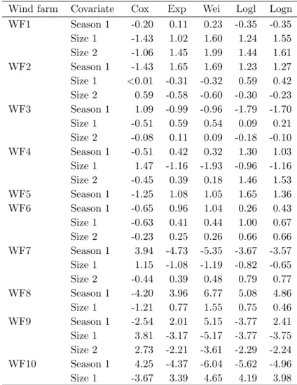
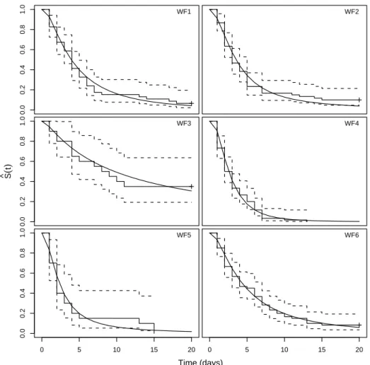
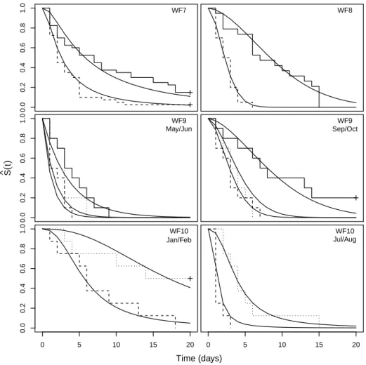
Discrimination Between Parametric Models 39 affected significantly by season and body size factors in 6 out of the 10 wind farms (WF1 to WF6). In WF7 and WF8 wind farms, season proved to have a significant effect (p < 0.001) and in WF9 and WF10 wind farms, both covariates had a significant effect on the removal times (p < 0.001). Although the described plotting procedures were used for all the 10 analyzed data sets, plots based on the linearization of the survivor function are shown only for WF1 to WF6 wind farms data sets (in which covariates were found not to affect significantly the removal times) and plots superimposing the empirical and the adjusted models are used to illustrate the adequacy of the models accounting for dependency on explanatory variables (WF7 to WF10).

AIC and BIC statistics showed a very strong agreement between them, pointing to the same model selection in all the 10 analyzed data sets. Hence, we refer here only the results according to the AIC. For the WF1, WF3, WF4 and WF6 wind farms, the AIC was found to be the lowest for the log-normal model, while the best ﬁtting model was the log-logistic for the WF2 and WF5 wind farms. However, diﬀerences between AIC values for the log-logistic and log-normal models were minimal, suggesting similar model adjustment, which, in fact, was expected, since these models are very similar. Consequently, inferences based on either model will be, in this case, very similar.

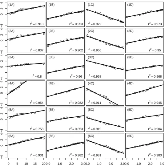
Plots based on the linearization of the survivor function (Figure 4.1) show that the exponential model has the poorest fit in all six wind farms (smaller coefficients of determination), which reflects the rel-ative inadequacy of the exponential distribution to model removal

(54)

40 _{Discrimination Between Parametric Models} times under this context. The remaining parametric models give fairly good approximated linear relationships, with slight diﬀerences between them. The coeﬃcients of determination point to the log-logistic and the log-normal models as the most suitable, matching the results from AIC. For the WF4 wind farm the best linear relationship was found for the Weibull model.

Comparisons between the four fitted models, based on plots shown in Figure 4.2, seem hard as differences between the models are almost eye imperceptible. Hence, model selection based on these type of plots is risky and can be misleading. The relative goodness-of-fit measures assume, therefore, a specially important role in this context.

Regarding the WF7 and the WF8 wind farms, lowest AIC values were found for the log-normal and the Weibull models, respectively, sug-gesting these models as the most suitable to model carcass removal times at these wind farms. For the WF9 and WF10 data, AIC in-dicates the Weibull and the log-logistic models as the most suitable. However, AIC values were very similar for the Weibull, the log-logistic and the log-normal models, which, in fact, was expected given the minor diﬀerences between corresponding plots displayed in Figure 4.2.

The analysis of the residuals revealed no major problems with any of the best ﬁtted models.

(55)

Discrimination Between Parametric Models 41 −4 0 2 4 (1A) r2=0.913 (1B) r2=0.953 (1C) r2=0.979 (1D) r2=0.973 −4 0 2 4 (2A) r2=0.837 (2B) r2=0.902 (2C) r2=0.956 (2D) r2=0.95 −4 0 2 4 (3A) r2=0.8 (3B) r2=0.96 (3C) r2=0.968 (3D) r2=0.968 −4 0 2 4 (4A) r2=0.954 (4B) r2=0.982 (4C) r2=0.911 (4D) r2=0.945 −4 0 2 4 (5A) r2=0.758 (5B) r2=0.853 (5C) r2=0.919 (5D) r2=0.904 0 5 10 15 20 −4 0 2 4 (6A) r2=0.931 0.0 1.0 2.0 3.0 (6B) r2=0.982 0.0 1.0 2.0 3.0 (6C) r2=0.981 0.0 1.0 2.0 3.0 (6D) r2=0.983

Figure 4.1: Plots based on the linearization of the survivor function for the inspection of the ﬁtted parametric survival models adequacy in 1 - WF1, 2 - WF2, 3 - WF3, 4 - WF4, 5 - WF5 and 6 - WF6 wind turbine sites, regarding A - exponential, B - Weibull, C - log-logistic and D - log-normal ﬁtted models

4.1.5 Concluding remarks

While we focus on wind farms wildlife fatalities, the methodological approach proposed and investigated herein is, nonetheless, broadly

(56)

ap-42 _{Discrimination Between Parametric Models} 0.0 0.4 0.8 (7A) (7B) (7C) (7D) 0.0 0.4 0.8 (8A) (8B) (8C) (8D) 0.0 0.4 0.8 (9A) Sep/Oct (9B) Sep/Oct (9C) Sep/Oct (9D) Sep/Oct 0.0 0.4 0.8 (9A) May/Jun (9B) May/Jun (9C) May/Jun (9D) May/Jun 0.0 0.4 0.8 (10A)

Jul/Aug Jul/Aug(10B) Jul/Aug(10C) Jul/Aug(10D)

0 5 10 15 20 0.0 0.4 0.8 (10A) Jan/Feb 0 5 10 15 20 (10B) Jan/Feb 0 5 10 15 20 (10C) Jan/Feb 0 5 10 15 20 (10D) Jan/Feb Time (days) S ^ (t )

Figure 4.2: Empirical (step functions) and ﬁtted parametric survivor functions at 7 - WF7 (step solid line: Jan/Feb and step dashed line: Jul/Aug), 8 - WF8 (step solid line: May/Jun and step dashed line: Sep/Oct), 9 - WF9 (step solid line: small size carcasses, step dashed line: medium size carcasses and step dotted line: large size carcasses) and 10 - WF10 (step dashed line: medium size carcasses and step dot-ted line: large size carcasses), regarding A - exponential, B - Weibull, C - log-logistic and D - log-normal models

plicable in many other contexts. In particular, we propose the used of the described methods in all the situations in which mortality by

(57)

Discrimination Between Parametric Models 43 collision with anthropogenic structures is a source of concern and, hence, whenever mortality estimation is mandatory. Among these sit-uations we emphasize wildlife mortality resulting from, e.g., collision with power lines (Ferrer et al., 1991; Hass et al., 2005), communica-tion towers (Ball et al., 1995) or cars on roads (Trombulak and Frissel, 2000) or from pesticide applications in agricultural systems (Kostecke et al., 2001). In these situations monitoring studies are conducted aiming to estimate the number of fatalities. In all of them, to cor-rectly estimate mortality it is important to consider carcass removal. For that reason it is a standard procedure to conduct carcass removal trials, collecting data regarding carcass removal times. As the estima-tion of this probability through the use of parametric models implies a distributional assumption, procedures used to check model adequacy are particulary important. Lawless (2003) underlines that

Often data are analyzed under a particular model sim-ply because (1) the model has been used before in similar situations, or (2) it ﬁts the data on hand. This does not imply any absolute validity of the model, and we should ask whether inferences change much if another similar ”plau-sible” model is used instead.

So, recognizing that the carcass persistence probability can, in fact, depend heavily on the model selected, this study proposes and applies a methodology to discriminate between competing survival models when analyzing data from carcass removal trials.

(58)

44 _{Discrimination Between Parametric Models} We found plotting procedures to be insufficient for model selection. Eye judgment of differences between the statistical models based on plots analysis was difficult. The analysis of the plots based on the linearization of the survivor function has the advantage of being in-terpreted in terms of coefficients of determination, leading to less am-biguous choices. Although plotting procedures do not discriminate sufficiently enough the fitted models, they enable to illustrate model adjustment after model choice. The use of the AIC allowed to choose the best relative fitted model.

The discrimination between the competitive parametric survival mod-els is strictly dependent on sample size and on censoring degree. Small sample sizes and higher censoring degrees lead, in general, to a less eﬃcient estimation and, therefore, the eﬃciency in discriminating

be-tween alternative competing models may be compromised. These

sources of error are still poorly explored. Hence, future work should be considered to evaluate extensively these eﬀects under the context of modeling carcass removal time for wildlife mortality assessment.