Portfolio construction and
risk management: theory
versus practice
Stefan Colza Lee
a,*and
William Eid Junior
a aFundação Getulio Vargas, São Paulo/SP, Brazil
Abstract
Purpose–This paper aims to identify a possible mismatch between the theory found in academic research and the practices of investment managers in Brazil.
Design/methodology/approach– The chosen approach is afield survey. This paper considers 78 survey responses from 274 asset management companies. Data obtained are analyzed using independence tests between two variables and multiple regressions.
Findings–The results show that most Brazilian investment managers have not adopted current best practices recommended by thefinancial academic literature and that there is a significant gap between academic recommendations and asset management practices. The modern portfolio theory is still more widely used than the post-modern portfolio theory, and quantitative portfolio optimization is less often used than the simple rule of defining a maximum concentration limit for any single asset. Moreover, the results show that the normal distribution is used more than parametrical distributions with asymmetry and kurtosis to estimate value at risk, among otherfindings.
Originality/value – This study may be considered a pioneering work in portfolio construction, risk management and performance evaluation in Brazil. Although academia in Brazil and abroad has thoroughly researched portfolio construction, risk management and performance evaluation, little is known about the actual implementation and utilization of this research by Brazilian practitioners.
Keywords Risk, Performance evaluation, Portfolio construction
Paper typeResearch paper
1. Introduction
Many new methods and concepts have emerged infinancial portfolio construction, risk management and performance evaluation since Markowitz’s (1952) pioneering work. The use of the variance, or standard deviation, of returns as a proxy for investment risk has been questioned, and alternative risk measures have been proposed, according toRom and Ferguson (1994);Roman and Mitra (2009)andAraújo and Montini (2015). The use of the original sample covariance matrix to estimate the risk of an asset portfolio has also been questioned, according toChanet al.(1999)and
© Stefan Colza Lee and William Eid Junior. Published inRAUSP Management Journal. Published by Emerald Publishing Limited. This article is published under the Creative Commons Attribution (CC BY 4.0) licence. Anyone may reproduce, distribute, translate and create derivative works of this article (for both commercial and non-commercial purposes), subject to full attribution to the original publication and authors. The full terms of this licence may be seen at http://creativecommons.org/ licences/by/4.0/legalcode
The authors are grateful to Daniela Gama, Brielen Madureira, Vivian Lee, Tiago Giorgetto, Edison Flores, José Miguel Burmester, members of the Centro de Estudo de Finanças of FGV and the questionnaire respondents.
Portfolio
construction
345
Received 17 November 2016 Accepted 18 July 2017
RAUSP Management Journal Vol. 53 No. 3, 2018
pp. 345-365
Emerald Publishing Limited 2531-0488 DOI10.1108/RAUSP-04-2018-009 The current issue and full text archive of this journal is available on Emerald Insight at:
Santos and Tessari (2012). Not even the use of quantitative methods to optimize portfolios or to allocate resources among different asset classes has been spared from criticism (DeMiguelet al.(2009).
Given the vast academic literature that proposes, explains and details numerous methods for portfolio construction and risk management and performance evaluation, the following central research question is addressed in this paper: among the major quantitative techniques for portfolio construction, risk management and performance evaluation suggested by the international and Brazilian academic literature, which ones are actually adopted by financial market practitioners? The main objective is to identify possible differences between what is taught in classrooms or discussed in academic conferences and what is involved in the day-to-day practice of asset managers and to determine whether a mismatch exists.
In addition to the central research question, the present work aims to compare Brazilian data with European data to inform us about the degree of globalization of the Brazilian asset management industry. Another specific goal is to check the existence of different practices among subgroups in the industry, such as companies of foreign and Brazilian origin, and to investigate the determinants of optimization and risk budgeting.
To achieve these objectives, we conduct a literature review and obtain 78 responses from a field survey with 274 asset management companies. The number of respondents is considerable, especially given the limited universe of professional asset management companies and the difficulty of extracting information from participants in a highly competitive and results-oriented segment. Thefield survey used an online questionnaire similar to that applied byAmencet al.(2011)in Europe. To analyze the data, the present paper uses Pearson’s chi-square independence test, multiple regressions using ordinary least squares (OLS) and a probit model.
According toAmencet al.(2011), little is known about the dissemination and use of academic research findings among investment professionals. Survey-based papers can assist in guiding and developing empirical studies and new theories by academics and can alert practitioners of research-informed recommendations that have not yet been adopted, according toGraham and Harvey (2001). However, similar surveys for Brazil have not been found, thus confirmingAmencet al.’s study (2011)and justifying this paper.
This paper is divided intofive sections, including the introduction. In Section 2, based on the existing theory, we formulate hypotheses regarding the practices of investment managers. Section 3 describes the empirical methodology of both thefield survey and data analysis. Section 4 presents the results, and Section 5 provides final remarks and suggestions for future studies.
2. Literature review and Hypotheses 2.1 Measuring market risk
This paper uses the definition of market risk proposed by Dowd (2002): it is the risk resulting from changes in prices, such as changes in public companies’share quotes, and rates, such as the interest rate and exchange rate. Two ways to quantify this risk are using variance and using downside risk.
Markowitz (1952), who used the variance of returns as a measure of risk, was one of the pioneers in proposing a quantitative methodology for portfolio construction. His work, along with that ofSharpe (1964)andLintner (1956), generated discussions and publications that formed the modern theory of portfolios.
RAUSP
53,3
Rom and Ferguson (1994) and Roman and Mitra (2009) argued in favor of more appropriate risk measures for asymmetric distributions of returns, so-called downside risk metrics. They proposed a new paradigm for portfolio construction and risk management, made possible by computational advances and made necessary by the increasing use of derivatives in portfolios. They termed this new paradigm the post-modern portfolio theory.
Among the downside risk metrics, semivariance, proposed by Markowitz (1959), is equivalent to the variance using only below-average returns.Bawa (1975)andFishburn (1977)subsequently developed lower partial moments (LPM). Series can be described using thefirst four moments: mean, standard deviation, kurtosis and asymmetry. LPM is for moments what semivariance is for variance, as LPM is based on only one side of the distribution.
While LPM and semivariance focus on returns below a target or the average, respectively, the other downside risk metrics, value at risk (VaR) and conditional value at risk (CVaR) or expected shortfall (ES) focus on extreme negative returns or tail risk. According toDowd (2002), the VaR is the maximum likelyfinancial loss within a given period and confidence interval provided that there is no certainty of an extreme adverse event. The CVaR ofRockafeller and Uryasev (2000)is the expected loss conditional on the occurrence of an extreme adverse event.
Empirical studies comparing and ranking different risk metrics usually consider the out-of-sample return of portfolios optimized for various risks but with the same return in the sample period. Brazilian studies indicate that LPM-optimized portfolios generally yield the best results, independent of the normality of the distribution of returns; see Andrade (2006)andAraújo and Montini (2015). In light of the literature,H1, to be tested is as follows:
H1. Post-modern theory is used more than the modern theory in performance evaluation and in optimization and risk budgeting with absolute risk.
Risk budgeting is a risk management practice in which the portfolio is changed whenever necessary to contain the predicted risk within predetermined limits. Examples of absolute risk are variance, semivariance and VaR.
In addition to the absolute risk metrics described above, relative risk metrics, which measure the variability of the differences between portfolio returns and a benchmark, are essential for the evaluation of investment managers; seeRoll (1992). Relative risk metrics are of interest both to passive portfolio managers who aim to replicate the returns of an index or benchmark and to active portfolio managers. Metrics such as tracking error may be used to verify with statistical significance whether a fund with active management is adding value relative to a passive portfolio:
TEp¼
ffiffiffiffiffiffiffiffiffiffiffiffiffiffiffiffiffiffiffiffiffiffiffiffiffiffiffiffiffiffiffiffiffiffiffiffiffiffiffiffiffiffi 1
N 1 X
N
n¼1
Dn D
2
v u u
t
ffiffiffiffi T p
(1)
whereTEpis the tracking error,Nis the number of observations,nis the index of the sum,T
is the sample frequency,Dn= Rportfolio,n Rbenchmark,nandDis the average of the return
differences. Thus, we have:
H2. The use of relative risk is independent of whether the asset manager has passive indexed funds.
Portfolio
construction
2.2 Covariance matrix estimation
The estimation of portfolio risk typically uses the covariance matrix, which contains the variance of each asset, as well as the covariance for all combinations of two assets, according to Dowd (2002). The covariance matrix is a key part of both portfolio optimization, which aims to obtain the optimal weights of assets, and risk management, which aims to estimate the expected risk of a portfolio or the portfolio’s VaR, as inScherer (2002).
RiskMetrics, proposed by Guldimann et al. (1996), uses an exponentially weighted moving-average approach and essentially has only one difference relative to the sample covariance matrix; that is, most recent observations receive greater weight. An exponentially weighted moving-average or EWMA conditional covariance matrix Rt is given by:
Rt¼ð1 lÞRt 1R0t 1þlRt 1 (2)
whereRtis the vector of asset returns at time t,l is the decay factor, 0<l <1 and the
recommended value isl= 0.94 for daily data.
Stein (1956)showed that the individually estimated sample mean is not a good estimator of the population mean when it has a multivariate normal distribution. The implication is that in portfolio construction, the sample-based covariance matrix may have estimation errors, although it is not biased. In the same paper, the author suggests using a statistical method to reduce estimation errors, which results in the use of an estimator constructed from the unbiased estimator and a biased and structured estimator, which is subjective and based on previous knowledge and experience.
According toLedoit and Wolf (2003), the shrinkage method for the covariance matrix is based on the work ofStein (1956) and entails the adjustment of the sample covariance matrix, which typically presents more extreme coefficients, toward afixed target known as the biased estimator, which ideally has more central values.Frost and Savarino (1986)and Jorion (1986)initially applied shrinkage in the construction of portfolios, but the method did not become practical and feasible until the work ofLedoit and Wolf (2003). We can represent the covariance matrix as:
Rt¼aFtþð1 aÞR^t (3)
where Ftis thefixed target or biased estimator,a[[0,1] and can be interpreted as the weight given to the biased estimator andR^tis the sample covariance matrix.
An alternative way to use the methods suggested above for the covariance matrix involves the use of factors and is based on the theoretical framework such asRoss’s (1976) arbitrage pricing theory (APT) and empirical studies such as those ofFama and French (1992). In APT, the excess return of an asset is:
Ri Rf ¼
X
k
n¼1
bnfn Rf (4)
where there are k systematic risk factors,Riis the rate of return of asset i,Rfis the risk-free
rate,bnis the sensitivity or load of asset i on risk factornandfnis the risk premium of
factorn. Assuming that the factors are not correlated with the residual return and that the residual returns are not correlated, the covariance matrix for N assets according toChan
et al.(1999)is:
RAUSP
53,3
R¼BXB0þD (5)
whereBis the factor sensitivity matrix,Xis the covariance matrix of the factors andDis a diagonal matrix containing the residual variances of the return.
Statistical factors are also known as implicit factors, as they are hypothetical variables constructed to explain the movement of a set of time series of returns; seeDowd (2002). Principal component analysis or factor analysis (FA) can be used to identify factors, and both of these quantitative methods can identify independent sources of movement. One of the advantages of using implicit factors in calculating the covariance matrix is to reduce the computational burden since risk factors are independent and a small number of factors are sufficient to achieve high explanatory power; see Alexander (2001) and Amenc and Martellini (2002).
In addition,Engle (1982) andBollerslev (1986) introduced the univariate generalized autoregressive conditional heteroskedasticity (GARCH) model. Some versions of the multivariate model can dynamically estimate expected and conditional variance and covariance for portfolio assets, and these approaches are recommended when asset volatility is inconsistent over time.
Empirical studies such as those ofSantos and Tessari (2012)andBeltrame and Rubesam (2013) point out that the covariance matrix shrinkage method, which combines sample covariance with structured estimators, yields the best results among all the methods. The third test of theory versus practice thus involves testing.
H3. The method most commonly used to determine the covariance matrix is shrinkage.
Studies in Brazil, such asSantos and Tessari (2012), show that minimum variance portfolios obtained through quantitative optimization using the sample covariance matrix, RiskMetrics, explicit factors and GARCH generally have higher returns than an equal-weighted portfolio and a market cap equal-weighted portfolio. Although authors such asDeMiguel
et al. (2009)obtained different results when studying listed companies in the USA, we
considerH4as follows:
H4. Investment managers use optimization methods more than the simple rule of establishing a maximum concentration limit per asset.
We do not detail the specific methodology used to optimize portfolios for a risk metric given a covariance matrix. Basically, this entails the optimization of a function subject to constraints. The methodology for portfolio optimization can be found in the studies of Roman and Mitra (2009)andAraújo and Montini (2015).
According toScherer (2002), managers who are constrained by a risk budget should perform portfolio optimization. The selection of assets and definition of their weights through optimization indicate to managers the optimal portfolio for the pre-established risk limit. Thus, we have:
H5. Investment managers who comply with a risk budget tend to perform portfolio optimization more than those who do not.
2.3 Distribution of returns
According toRoman and Mitra (2009), research on return distributions is as important as the study of risk measures and covariance matrices in maximizing returns or minimizing
Portfolio
construction
risks in a portfolio. The practical implications are better estimates of the parameters for the optimization offinancial models, such as the mean and variance optimization of Markowitz or thecapital asset pricing model(CAPM), and for option pricing models, according toLeal and Ribeiro (2002).
One way to test the suitability of a return distribution is to use the VaR and the Kupiec failure ratio test, which essentially consists of counting the number of losses above the established VaR using out-of-sample testing.
Historical VaR assumes that the distribution of future returns is non-parametric and is based exclusively on historical data or, in other words, that the past provides all the information and the future probability distribution will be equal to the past distribution. The Monte Carlo VaR assumes that future returns will follow a known stochastic process and a non-parametric distribution. To obtain historical or Monte Carlo VaR at thefifth percentile (or a 95 per cent confidence interval), the historical or simulated returns are sorted in ascending order, and the return at thefifth percentile is the estimated VaR.
The simplest parametric VaR assumes that future returns will follow a normal, or Gaussian, parametric distribution that can be estimated with only two parameters: the mean and the expected standard deviation of the returns.
VaR with higher moments considers the existence of kurtosis, asymmetry or both in the distribution and is a more appropriate parametric method when returns do not follow a normal distribution. According to Dowd (2002), one way to consider kurtosis in a distribution is through the Student’s t distribution, which has a kurtosis equivalent to 3 (y 2)/(y 4), whereycan be chosen based on the expected kurtosis of future returns such that 5<y<9.
Extreme value theory (EVT) provides a basis for modeling events with significant economic consequences and very small probabilities of occurring. The generalized extreme value distribution is parametric and may be used to build the worst-case scenario in ten years in the equity market or the probability of the euro-dollar exchange rate appreciating more than 20 per cent in a week.
Brazilian and international empirical studies such asCassettari (2001),Leal and Ribeiro (2002) and Arraes and Rocha (2006) show that financial asset returns demonstrate asymmetry and kurtosis, and therefore, VaR with a normal distribution is not the most appropriate method.H6will test whether the methods suggested by empirical studies in academia are the most frequently used by practitioners but will focus on return distributions:
H6. investment managers use parametric distributions, such as EVT or distributions with higher moments, more than they use a normal distribution to estimate VaR.
2.4 Management of estimation risk
Scherer (2002b)pointed out that the portfolio optimization process suffers from error maximization since assets with higher returns, low risk or low covariance tend to be chosen. Extreme results have a higher probability of estimation errors; in other words, they tend to be unsustainable in the long term. In addition, there is a consensus among scholars about the inability to predict future asset returns and a belief that the optimization process is very sensitive to differences in the expectation of future returns (Michaud, 1989). Some alternatives proposed to address estimation risk are presented below.
RAUSP
53,3
The Monte Carlo resampling of Michaud (1989) and Michaud and Michaud (2008) typically uses the draw-with-replacement method to simulate asset returns based on their historical distribution. Usually, the simulation is performed hundreds of times and for all assets to test investment strategies.
Bayesian models and the Black Litterman model–seeJorion (1986)andBlack and Litterman (1992) – allow us to add subjective individual convictions to the quantitative financial models. The model will make recommendations after confidence levels for the quantitative model and the subjective individual conviction are determined.
A different strategy to reduce estimation risk involves maintaining a portfolio with the lowest expected risk. The minimum variance portfolio depends only on the covariance estimation and is subject to a more moderate estimation error than other mean-variance portfolios are; see the studies ofChanet al.(1999);DeMiguelet al.(2009) and Caldeira et al. (2013). Given the importance of adopting techniques to manage estimation risk, we thus test:
H7. Estimation risk management methods are more commonly used than the simple rule of imposing a maximum concentration per asset.
2.5 Performance evaluation
The use of risk-adjusted returns to evaluate performance was proposed at nearly the same time as the CAPM model.Treynor (1965);Sharpe (1966)andJensen (1968)proposed risk-adjusted performance measures based on the theoretical framework of Markowitz’s mean-variance model. The desire for a portfolio optimization method to account for market risk and investment analysts’opinions ledTreynor and Black (1973)to create a ratio that would later be known as the information ratio. Last on our list of performance measures that are based on the modern portfolio theory is theModigliani and Modigliani (1997)ratio, which can be interpreted as the return that a fund would have if its risk were equivalent to market risk.
Among the performance metrics that are based on downside risk or post-modern portfolio theory, theSortino and Van Der Meer (1991)ratio and the return relative to the VaR are worth noting. In the table below, it is important to note that for the Sortino ratio, an investor can replace the risk-free return with a minimum acceptable return; the LPM can replace the semivariance, and the investor can define the degrees of freedom.Dowd (2000) proposed the return relative to VaR and defined it as the return above the risk-free rate divided by the portfolio’s VaR (Table I).
Estimating the alpha of a portfolio is not restricted to the method proposed byJensen (1968), where the alpha is the portfolio return adjusted for the market risk incurred. According toBailey (1992), the simplest method to estimate alpha is to compare the returns obtained with other similar funds.Fama and French (1992)suggested capturing alpha through multifactor models that consider, for example, size and value factors. Performance attribution and style analysis facilitate the decomposition of excess returns into various components. These components may include, for example, asset class allocation and stock selection or allocation to risk factors (BARRA, 1990;Sharpe, 1992).
H8refers to the popularity of risk-adjusted returns:
H8. Risk-adjusted returns are used more than unadjusted returns.
Portfolio
construction
3. Empirical methodology
To test the hypotheses, we collected data via online questionnaires hosted on the website of the Centro de Estudos em Finanças CEF of Fundação Getúlio Vargas’ Business Administration School. Invitations and links were sent to key executives, portfolio and risk managers representing 274 asset management companies between August and September 2015. To increase the number of responses, follow-up telephone calls were made to the managers. We obtained telephone numbers and email addresses from the CEF database.
The questionnaire had a total of 3 sections and 17 questions that required the analysis of 65 non-mutually exclusive responses. The questionnaire is based on the work ofAmenc
et al.(2011), who surveyed investment managers in Europe in 2007 on portfolio management
and performance evaluation. Although based on a previous survey, a pre-test of the questionnaire was conducted with a group of investment managers with the objective of evaluating the terminology, the clarity of the questions and the average response time, with the main goal of improving the questionnaire.
All questionnaires, according toGraham and Harvey (2001), are subject to potential problems; for example, the responses may not reflect respondents’actions. One concern regarding this work is that some respondents could omit certain information for fear of being copied. Therefore, all the questions were obligatory, except for some identification data: name and email, name and origin of the asset management company and whether the asset management company is affiliated with a bank. Ten of the respondents chose not to identify themselves.
In the present study, all variables of interest are categorical, the majority being binary, with only two categories of responses, such as“uses”and“does not use”. Thefirst type of test was the independence test of two variables, which was used to compare categorical Table I.
Performance metrics
Name Risk metric Portfolio theory Formula
Absolute return No risk adjustment None Rp
Excess return on benchmark No direct risk adjustment None Rp Rb
Sharpe ratio Standard deviation Modern* Rp Rf
sp
Treynor ratio Beta CAPM Modern Rp Rf
bp
Jensen’s alpha Beta CAPM Modern Rp (Rfþbp(Rm Rf)
Information ratio Standard deviation of
residual ortracking error
Modern* ap
s«p
Modigliani and Modigliani–M2 Beta CAPM Modern* Rp Rf
sp
sm Rf
Sortino ratio Semivariance Post-modern RpffiffiffiffiffiffiffiffiRf
SVp
p
Return relative to VaR VaR Post-modern Rp Rf
VaR
Note:*The empirical tests reported in Section 4 compare the adoption of these performance measures based on the modern theory of portfolios with the adoption of the Sortino index and the return relative to VaR
RAUSP
53,3
responses between two groups of the same sample or population. We performed independence tests, for example, to compare the rates of utilization of different portfolios and risk management methods. The statistic of the independence test, more specifically of the chi-square test, of Pearson, is given byx2(Table II):
eij¼
Total of Line i
ð ÞðTotal of Column jÞ Size of the Sample Nð Þ
x2¼X
i
X
j
fij eij
2
eij
whereeijis the expected frequency based on the independence hypothesis for the category in
Rowi and Columnj of the contingency table and fij is the frequency observed for the
category in Rowiand Columnjof the contingency table. When we analyze two groups and binary responses, the test statistic has approximately a chi-square distribution for large samples with one degree of freedom.
Notably, using a Z-test is preferable when one wishes to analyze differences in the proportions of two different populations. An example is the comparison of proportions verified in the present research carried out in Brazil, with the proportions verified in the research ofAmencet al.(2011)in Europe. TheZ-test uses two normal distributions rather than independence tests. In cases where the alternative hypothesis is the inequality of proportions and where the chi-square distribution has one degree of freedom, both theZ-test and the chi-square test produce exactly the same p-values and the same statistical inferences.
Agresti (1996)suggested the use of Fisher’s exact test, which is based on an exact distribution, for statistical inference when the sample is small and the expected value is less than five in any of the categories of the contingency table. To ensure robustness, Fisher’s exact test was performed to confirm the chi-square test results, and because we did notfind significant differences, we omitted the results of Fisher’s exact tests.
The second type of test used multiple regressions to reveal the determinants of the use of quantitative optimization and risk budgeting by investment managers. OLS regressions, known as linear probability models when dependent variables are binary, can be used to reveal causal relationships, according toAngrist and Pischke (2009). We use the probit model for robustness tests. In both regressions, our interest lies mainly in the probability that an observation with particular characteristics will fall into one of two categories:
P yð ¼1jx1;x2;. . .;xnÞ (6)
Table II. Pearson’s chi-square independence test statistic
Contingency table Column variable (groups)
Line variable (answers) 1 2 Total
1: Uses X1 X2 X
2: Does not use n1 X1 n2 X2 n X
Total n1 n2 N
Portfolio
construction
where y is the dependent variable and binary indicator andx1is the set of explanatory
or independent variables. In the regressions, it is assumed that the probability of response is linearly determined by a set of parameters, and in a probit model, it is also assumed that the probability of response adheres to a standard normal cumulative distribution function. All tests and regressions were conducted using the software Stata version 13.
4. Analysis and discussion of results
4.1 Descriptive statistics and comparison of results with European data
There were 78 respondents; 21 per cent of the asset management companies had a foreign origin, and 29 per cent were affiliated with a bank. Regarding the size of the assets under management, 18 per cent of the respondents play an active role in the management of up to R$250m, 27 per cent between R$250m and R$1bn, 20 per cent between R$1bn and R$5bn and 35 per cent above R$5bn. Regarding the type of managed fund, 62 per cent have active equity funds, 21 per cent indexed equity funds, 26 per cent short-term government bond funds orfundos DI, 47 per centfixed income funds, 73 per cent hedge funds orfundos multimercadosand 15 per cent other funds.
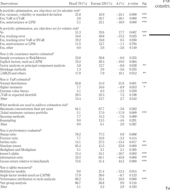
InTable III, we present a comparison of the results obtained with those ofAmencet al. (2011), as well as thep-value of the equality of proportions test, which will, in this case, be identical to thep-value of the chi-square test, as explained in Section 3 of the paper.
4.2 Adoption of modern and post-modern theory
Three independence tests were performed to compare investment managers’adoption of the modern theory with that of post-modern theory. No statistically significant differences in risk management were found, specifically in the use of risk budgeting; 51.3 per cent are based on the modern theory and 59.0 per cent on the post-modern theory. Statistically significant differences in favor of the modern portfolio theory compared with post-modern theory were found:
in the construction of portfolios (21.8 per cent versus 6.8 per cent respectively) and
in performance evaluation (80.8 per cent versus 35.9 per cent, respectively).
Despite the results of academic studies such asAraújo and Montini (2015), the results reported inTable IVlead not only to the rejection ofH1, but also to the conclusion that the modern theory remains the dominant paradigm among practitioners.
We testedH1 in several subsamples: large asset management companies, with over R$1bn in assets under management, and small companies; companies with hedge funds and without; companies affiliated with banks and those that are independent; and companies with (a) one or two and three or (b) more types of funds. The results reported inTable V rejectH1for all subgroups in the sample as they are similar to the ones obtained for the full sample.
4.3 Determinants of relative risk budgeting and portfolio optimization
The importance of relative risk and return for Brazilian investment managers is evident: 75.6 per cent target a return above the benchmark, 64.1 per cent and 48.7 per cent perform, respectively, budgeting and portfolio optimization with relative risk. For comparison purposes, 65.4 per cent aim for the absolute return, and 55.1 per cent and 25.6 per cent perform budgeting and portfolio optimization with absolute risk. We conduct OLS and probit regressions to better understand the determinants of the use of
RAUSP
53,3
Table III. Comparison of selected responses for Brazil vs Europe
Observations Brazil 78 (%) Europe 229 (%) D(%) p-value Sig
In portfolio optimization, are objectives set for absolute risk?
Yes, variance, volatility or standard deviation 21.8 45.9 24.1 0.000 ***
Yes, VaR or CVaR 2.6 50.7 48.1 0.000 ***
Yes, semivariance or LPM 5.1 23.1 18.0 0.000 ***
In portfolio optimization, are objectives set for relative risk?
No 51.3 33.6 17.7 0.007 ***
Yes, tracking error 34.6 49.8 15.2 0.025 **
Yes, tracking error VaR or BVaR 19.2 18.8 0.5 0.930
Yes, semivariance or LPM 11.5 12.7 1.1 0.794
Yes, other 0.0 2.6 2.6 0.149
How is the covariance matrix estimated?
Sample covariance or RiskMetrics 53.8 59.8 6.0 0.355
Explicit factors, such as CAPM 19.2 29.3 10.0 0.084
Factor analysis or principal component analysis 3.8 12.7 8.8 0.028 **
Shrinkage methods 1.3 3.9 2.6 0.255
GARCH and others 17.9 7.9 10.1 0.012 **
How is VaR estimated?
Normal distribution 62.8 41.0 21.8 0.001 ***
Higher moments 7.7 16.6 8.9 0.053 *
Extreme value theory 5.1 8.3 3.2 0.359
CVaR or expected shortfall 29.5 22.3 7.2 0.198
Other 15.4 12.7 2.7 0.542
What methods are used to address estimation risk?
Maximum concentration limit per asset 64.1 67.7 3.6 0.562
Global minimum variance portfolio 5.1 17.0 11.9 0.009 ***
Bayesian methods 7.7 15.3 7.6 0.089
Resampling 9.0 13.5 4.6 0.291
Other 9.0 6.1 2.9 0.387
How is performance evaluated?
Sharpe ratio 78.2 77.3 0.9 0.868
Treynor ratio 7.7 10.9 3.2 0.414
Sortino ratio 14.1 27.5 13.4 0.017 **
Absolute return 65.4 41.5 23.9 0.000 ***
Modigliani and Modigliani 5.1 3.1 2.1 0.395
Jensen’s alpha 15.4 34.1 18.7 0.002 ***
Information ratio 19.2 65.1 45.8 0.000 ***
Excess return relative to benchmark 75.6 31.4 44.2 0.000 ***
How is alpha measured?
Multifactor models 9.0 21.4 12.4 0.014 **
Single-factor models (such as CAPM) 17.9 26.6 8.7 0.123
Performance attribution or style analysis 69.2 35.4 33.9 0.000 ***
Peer group analysis 66.7 56.8 9.9 0.124
Other 5.1 2.2 2.9 0.183
Notes:Thep-values provided are from Pearson’s chi-square test with one degree of freedom. The null hypothesis is the equality of proportions, and the alternative hypothesis is inequality. We reject the null hypothesis atp<0.01 (***);p<0.05 ( **) andp<0.1 (*)
Portfolio
construction
relative risk and to testH2. The same approach was used to analyze the determinants of portfolio optimization and to testH5; seeTable VI.
In Models (1) and (2) inTable VII, the dependent variable is binary with a value of 1 (one) when the manager has a budget for relative risk and 0 (zero) when there is no such budget. In the other models, the dependent variables are also binary and take a value of one when the method is adopted and zero otherwise. The dependent variable is portfolio optimization with relative risk in Models (3) and (4) and is optimization with absolute risk in Models (5) and (6). Models (1)-(4) will be used to testH2and Models (3)-(6) to test H5.
The independent variables are as follows: indexed equity funds, which is an indicator variable for whether or not the manager has passive indexed equity funds; active equity funds; large, if the assets under management are above R$1bn; foreign, Table V.
Results ofH1 chi-square tests on subsamples
Subsample Obs
T1a T1b T1c
p-value Sig p-value Sig p-value Sig
Large 43 0.822 0.024 ** 0.000 ***
Small 35 1.000 0.101 * 0.001 ***
With hedge funds 57 0.338 0.003 *** 0.000 ***
Without 21 0.753 1.000 0.002 ***
Banks 20 0.490 0.633 0.010 **
Independent 46 0.835 0.036 ** 0.000 ***
1 or 2 funds 32 0.035 ** 0.03 ** 0.002 ***
3 or more funds 46 0.676 0.079 * 0.000 ***
Total 78 0.334 0.006 *** 0.000 ***
Notes:Thep-values provided are from chi-square tests of independence. The null hypothesis is equal use of modern and post-modern theory. T1a, T1b and T1c, respectively, address absolute risk budgeting, absolute risk optimization and performance evaluation. We reject the null hypothesis atp<0.01 (***);p<
0.05 (**);p<0.1 (*) Table IV.
Description ofH1 variables, tests and results
ID Hypothesis Test Result
H1 Post-modern theory is used more than the modern theory in performance evaluation and in optimization and risk budgeting with absolute risk
Chi-square statistic
Hypothesis rejected based on tests in full sample and subsamples
Tests performed Hypotdeses p-value Sig Result
T1a Comparison of the proportions of respondents using modern (u1) and post-modern (u2) theory for absolute risk budgeting
h0:u1=u2 h1:u1>u2
0.334 H0Not Rejected
T1b Comparison of the proportions of respondents using modern (u1) and post-modern (u2) theory for portfolio optimization with absolute risk
h0:u1=u2 h1:u1>u2
0.006 *** H0Rejected
T1c Comparison of the proportions of respondents using modern (u1) and post-Modern (u2) Theory for performance evaluation
h0:u1=u2 h1:u1>u2
0.000 *** H0Rejected
RAUSP
53,3
which describes the origin of the asset management company; bank, if the asset management company is affiliated with a private or public bank; hedge funds, which includes any type of hedge fund; and budgeting with relative and absolute risk indicates whether the manager sets a risk budget or not.
With regard to the regression results, Models (1) and (2) indicate that the only variable that explains relative risk budgeting with statistical significance is whether investment managers have passive or indexed equity funds. The presence of an index equity fund increases the probability of using a relative risk budget by 29.6 per cent according to Model (1) OLS and by 31.2 per cent according to Model (2) probit. All marginal probabilities with probit are estimated considering the other variables at their mean.
Models (3) and (4) of Table VII have significant explanatory power. TheR2 and pseudoR2values for the probit model are 0.50 and 0.55, respectively. The models show
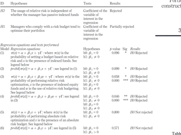
Table VI. Description ofH2 andH5variables, tests and results
ID Hypotheses Tests Results
H2 The usage of relative risk is independent of whether the manager has passive indexed funds
Coefficient of the variable of interest in the regression
Rejected
H5 Managers who comply with a risk budget tend to optimize their portfolios
Coefficient of the variable of interest in the regression
Partially rejected
Regression equations and tests performed
ModelRegression equations Hypotheses p-value Sig Results
(1) p(x) =aþb1xþgC: wherep(x)is the probability of setting a budget based on relative risk andxis the presence of indexed funds. See legend below
h0:b1= 0 h1:b1=0
0.096 * H0Rejected
(2) probit[p(x)] =aþb1xþgC: see legend in (1) h0:b1= 0
h1:b1=0
0.099 * H0Rejected
(3) p(x) =aþb1xþb2wþgC: wherep(x)is the probability of performing relative risk
optimization,xis the presence of indexed equity funds andwis the use of relative risk budgeting. See legend below
h0:b1= 0 h1:b1=0 h0:b2= 0 h1:b2=0
0.058 0.000 * *** H0Rejected H0Rejected
(4) probit[p(x)] =aþb1xþb2wþgC: see legend
in (3)
h0:b1= 0 h1:b1=0 h0:b2= 0 h1:b2=0
0.046 0.000 ** *** H0Rejected H0Rejected
(5) p(x) =aþb1vþgC: wherep(x)is the probability of performing absolute risk optimization andvis the presence of an absolute risk budget. See legend below
h0:b1= 0 h1:b1=0
0.800 H0Not rejected
(6) probit[p(x)] =aþb1vþgC: see legend in (5) h0:b1= 0
h1:b1>0
0.571 H0Not rejected
Notes:We reject the null hypothesis ofb= 0 atp<0.01 (***);p<0.05 (**);p<0.1 (*). The probit [p(x)] is a function or link that transformsp(x)into aZstatistic,ais the constant,b1andb2are the coefficients of interest,Cis the vector of control variables andgis the vector of coefficients of the control variables
Portfolio
construction
Independent variables
Dependent variables
Budgeting with relative risk Optimization with relative risk Optimization with absolute risk
(1) (2) (3) (4) (5) (6)
OLS PROBIT OLS PROBIT OLS PROBIT
Indexed equity funds 0.293* (0.173) 1.064* (0.644) 0.324* (0.168) 1.772** (0.889)
Active equity funds 0.0936 (0.138) 0.242 (0.369) 0.0300 (0.0902) 0.328 (0.455) 0.0231 (0.126) 0.0416 (0.392) Large 0.0646 (0.154) 0.157 (0.399) 0.0504 (0.104) 0.242 (0.448) 0.218* (0.126) 0.768* (0.462) Foreign 0.131 (0.132) 0.451 (0.477) 0.111 (0.141) 0.321 (0.622) 0.125 (0.153) 0.431 (0.485) Bank 0.130 (0.138) 0.367 (0.440) 0.0398 (0.0940) 0.531 (0.622) 0.0198 (0.128) 0.120 (0.465) Hedge funds 0.104 (0.131) 0.267 (0.361) 0.0915 (0.0825) 0.667 (0.499) 0.213** (0.104) 0.814* (0.455) Budgeting with relative risk 0.692*** (0.0914) 2.798*** (0.511)
Budgeting with absolute risk 0.0269 (0.106) 0.197 (0.348) Constant 0.530*** (0.142) 0.0618 (0.384) 0.0979 (0.0779) 1.516*** (0.492) 0.164 (0.141) 1.019* (0.526)
Observations 68 68 68 68 68 68
R2or probit’s pseudoR2 0.128 0.112 0.547 0.499 0.086 0.083
Notes:Robust standard errors are in parentheses. We reject the regression coefficientb= 0 atp<0.01 (***);p<0.05 (**);p<0.1 (*)
Table
VII.
Results
of
OLS
and
probit
regressions
RAUSP
53,3
that both the presence of indexed equity funds and the use of relative risk budgets explain optimization with relative risk. The presence of indexed funds increases the probability of relative risk optimization from 32.4 per cent in the OLS model (3) to 59.3 per cent in the probit model (4). The use of relative risk budgeting increases the probability of relative risk optimization from 69.2 per cent in the OLS Model (3) to 77.0 per cent in the probit model (4).
Two variables explain portfolio optimization with absolute risk with statistical significance, according to Models (5) and (6) inTable VII. Neither of them is absolute risk budgeting. Respondents with hedge funds are 21.3-20.2 per cent more likely than respondents without hedge funds to perform this procedure, according to the (5) OLS and (6) probit models, respectively. Respondents from large companies are between 21.8 per cent and 22.4 per cent less likely than those from small companies to perform absolute risk optimization, according to Models (5) and (6), respectively.
Before we conclude, it is important to make three brief technical notes and address some endogeneity concerns. First, the probit model assumes that the errors in the probability of response follow a normal distribution. The LPM model is more appropriate in our case because it is more robust to specification errors, and because the independent variables are all binary, all estimated probabilities will be within the range of [0,1]; seeAngrist and Prischke (2009). Second, the addition of relative risk budgeting and indexed equity funds as independent variables in the same regression generates multicollinearity because both are significantly correlated. This may increase the standard errors, making it harder to detect statistical significance in the regressors, but it will not bias the regression coefficients. Finally, the constants of regressions (1) to (6) theoretically indicate the probability of an asset management company performing a risk budget or optimization if the company is small and local; has no index, active equity or hedge funds; and is not affiliated with a bank. In practice, however, there is arguably considerable noise in the determination of the constants, and therefore, we will refrain from interpreting the constants.
It could be argued that the use of budgeting and optimization is what causes an asset management company to be large, which would create endogeneity due to reverse causality. The argument that investors seek risk-efficient portfolios is plausible and supported by studies in the USA.Ippolito (1992)andSirri and Tufano (1998)found a negative impact of risk on fundraising. However, only a marginal impact was found using US data, andMuniz (2015)found no impact at all in Brazil.
In Models (3)-(6) ofTable VII, it is unlikely that optimization causes the risk budget and that models suffer from reverse causality. It seems more plausible that investment managers who need to adhere to risk limits imposed by customers rely on optimization to help them determine the portfolio with the highest expected return for a certain amount of risk.
Finally, since the presence of an indexed or passive equity fund increases the probability of budgeting or optimizing with relative risk, the 16 respondents who had equity index funds are more likely to use relative risk than the remaining respondents, and thus,H2can be rejected.
As relative risk budgeting explains optimization with relative risk but absolute risk budgeting does not explain optimization with absolute risk, we can partially rejectH5. Risk budgeting was found to affect only optimization with relative risk, not optimization with absolute risk.
Although we do not have all the necessary elements, we will speculate on a possible explanation for the partial rejection ofH5. It may be the case that there are simple methods, such as limiting the maximum concentration per individual asset, that work sufficiently well
Portfolio
construction
for the management of absolute risk, but the same does not occur for the management of relative risk. An alternative, albeit longer, explanation is that it is well known that performance fees to asset management companies are generally tied to the excess return relative to the benchmark. Investment managers who do not perform optimization with relative risk may achieve lower excess returns, bring less revenue to the asset management company or fall outside of the pre-established risk limits. This would culminate in their dismissal, and investment managers who remain are those who optimize with relative risk. However, this may not be the case for portfolio managers who do not perform optimization with absolute returns, as performance fees are not usually linked to absolute returns.
4.4 Quantitative optimization and return distribution
Starting withH3, while only 1.3 per cent uses the shrinkage matrix, 34.6 per cent use RiskMetrics, the most popular method to produce a covariance matrix. Independence tests rejectH3. Despite the excellent results in empirical tests reported byLedoit and Wolf (2003) andSantos and Tessari (2012), even in Europe, the method is used by only 3.9 per cent of managers (Table III). Attributing this low adoption to a costly learning curve does not seem reasonable since models such as GARCH are possibly more complex and are used by 17.9 per cent of managers.
Imposing asset concentration limits is a simple and intuitive method but is relatively arbitrary and without scientific backing, according toAmencet al.(2011).H4tests whether this method is more popular than quantitative optimization. Of the respondents, 55.1 per cent performed optimization by absolute, relative risk or both, whereas 64.1 per cent set restrictions on asset concentration. The difference between the two proportions is not statistically significant, and we thus rejectH4.
Only 5.1 per cent of managers use EVT, 7.7 per cent use distributions with higher moments and 9.0 per cent use at least one of the two methods to estimate VaR. Because 62.8 per cent of the sample, a much higher percentage, uses the normal distribution, we can reject H6. See Table VIII. According to Cassettari (2001) and Leal and Ribeiro (2002), the preference for a normal parametric distribution is probably associated with simplicity and ease of use, but the asymmetry of the return distribution in the Brazilian market implies that simplification may lead to underestimation of the tail risk and may cause unpleasant surprises. Surprisingly, EVT and higher moments are more common in developed countries, where the return distribution resembles more a normal curve, than in Brazil (8.3 per cent and 16.6 per cent of respondents, respectively), according toTable III.
Investment managers in Brazil are much less likely to adopt the selected methods to manage estimation risk than are their counterparts in Europe. The respective values are 5.1 per cent versus 17.0 per cent that adopt minimum variance portfolios, 7.7 per cent versus 15.3 per cent that adopt Bayesian methods and 9.0 per cent versus 13.5 per cent that adopt resampling. SeeTable III. Only 24.4 per cent use some method to manage estimation errors, thus leading us to rejectH7. The results are robust for the subsample of 43 respondents who perform optimization with relative or absolute risk; see T7b inTable VIII.
4.5 Risk-adjusted versus unadjusted return
Previous tests suggest that there is a significant gap between best practices and current practices in the Brazilian asset management industry. One could argue that the comparison is of little use, as the ideas conveyed in academic publications will always be years ahead of the market. If best practices take years to be fully understood, disseminated and implemented and new ideas are constantly being created, then a gap should naturally be expected (Table IX).
RAUSP
53,3
The analysis of risk-adjusted returns was introduced in Treynor (1965); Sharpe (1966)and Jensen (1968)and cannot be considered new. Furthermore, it cannot be considered very complex, since in Europe, according toAmencet al.(2011), 77 per cent of managers use the Sharpe index and 65 per cent use the information ratio. They are the most commonly used metrics to evaluate performance in Europe, according to Table III.
Table IX. Description ofH8 variables, tests and results
ID Hypotheses Tests Results
H8 Risk-adjusted returns are used more than unadjusted returns
Chi-square statistic Hypothesis rejected
Tests performed Hypotheses p-value Sig Results
T8 Comparison of proportions of respondents using risk-adjusted (u1) and those using unadjusted (u2) returns
h0:u1=u2 h1:u1<u2
0.151 H0not rejected
Table VIII. Description ofH3, H4,H6andH7 variables, tests and results
ID Hypotheses Tests Results
H3 The method most commonly used to determine the covariance matrix is shrinkage
Chi-square statistic
Hypothesis rejected
H4 Investment managers use optimization methods more than the simple rule of establishing a maximum concentration limit per asset
Chi-square Hypothesis not rejected
H6 Investment managers use parametric distributions, such as extreme value theory or distributions with higher moments, more than the normal distribution to estimate VaR
Chi-square Hypothesis rejected
H7 Estimation risk management methods are more commonly used than the simple rule of imposing a maximum concentration per asset
Chi-square Hypothesis rejected
Tests performed Hypotheses p-value Sig Results
T3 Comparison of the proportions of respondents using shrinkage (u1) and those using RiskMetrics (u2) in determining the covariance matrix
H0:u1=u2 h1:u1<u2
0.000 *** H0Rejected
T4 Comparison of the proportions of respondents using quantitative optimization (u1) and those using maximum concentration per asset (u2) in the construction of portfolios
H0:u1=u2 h1:u1>u2
0.253 H0Not rejected
T6 Comparison of the proportions of respondents using extreme value theory or a distribution with upper moments (u1) and those using the normal distribution (u2)
H0:u1=u2 h1:u1<u2
0.000 *** H0Rejected
T7 Comparison of proportions of respondents using advanced estimation risk management methods (u1) and those using maximum concentration per asset (u2)
h0:u1=u2 h1:u1<u2
0.000 *** H0Rejected
T7b Same variables as T7. Test performed in the subsample of 43 respondents who perform portfolio optimization
h0:u1=u2 h1:u1<u2
0.000 *** H0Rejected
Note:We reject the null hypothesis atp<0.01 (***)
Portfolio
construction
Although it is relatively old and not very complicated concept, the risk-adjusted return is not as popular as the unadjusted return in Brazil, according to the survey, and we can thus rejectH8. Of the Brazilian managers, 91.0 per cent use absolute return or excess return relative to the benchmark; these are measures of return not directly adjusted for risk. In comparison, 83.3 per cent use at least one risk-adjusted return measure such as the Sharpe or information ratio.
5. Final remarks
This paper aims to identify a possible mismatch between the theory found in academic research and the practices of investment managers in Brazil. For this purpose, a bibliographical andfield survey was carried out with 78 respondents to a questionnaire posted online, out of a total of 274 asset management companies. This study may be considered a pioneering work in portfolio construction, risk management and performance evaluation in Brazil.
The results of the tests performed indicate that practice departs from theory in the country: of the eight hypotheses tested, we rejected seven hypotheses and partially rejected one hypothesis. One possible explanation is that few Brazilian academic studies consider transaction costs such as brokerage fees, bid-ask spreads and liquidity when studying the benefits of quantitative portfolio optimization.Santos and Tessari (2012)andCaldeiraet al. (2013), for example, considered three types of rebalancing, daily, weekly and monthly, which would generate very high turnover and cost.
Compared with investment managers in Brazil, those in Europe seem to be closer to the best practices propagated by academia. During the data collection process, some of the respondents mentioned that the low liquidity and quantity offinancial assets in Brazil did not justify the use of quantitative methods for portfolio construction. Notably, the European managers researched byAmencet al.(2011) represented companies with greater assets under management overall.
This work aims not only to suggest improvements to practitioners but also to help researchers better understand the reality in Brazil. As an example, althoughSantos and Tessari (2012)noted that the sample covariance matrix is seldom used by practitioners, only RiskMetrics is more popular than the sample covariance matrix.
Perhaps the most important contribution in this sense is that managers attach great importance to relative risk and return, but few empirical studies focusing on relative risk were found. In future work, we suggest that researchers compare optimized portfolios for tracking error, benchmark VaR and other optimization methods with relative risk. We also suggest studies that help determine how international diversification or the financial education of clients of asset management companies relates to the adoption of sophisticated methods for portfolio construction, risk management, and performance evaluation. Because the present study is limited in that it reflects the state of the industry in only a short time interval, longitudinal studies are suggested because they do not suffer from this restriction.
This paper also aimed to investigate the determinants of the risk budget and the optimization of portfolios. The only variable that significantly explained risk budgeting was the presence of passive or indexed equity funds. For portfolio optimization, the key explanatory variables differed depending on the type of risk: absolute or relative risk. While the presence of passive equity funds and risk budgeting increases the likelihood of relative risk optimization, the presence of hedge funds and assets under management of less than R$1bn increases the probability of absolute risk optimization.
RAUSP
53,3
References
Agresti, A. (1996),Introduction to Categorical Data Analysis, John Wiley & Sons, New York, NY. Alexander, C. (2001), Mastering Risk Volume 2 Applications, Financial Times/Prentice Hall,
London, pp. 21-38.
Amenc, N. and Martellini, L. (2002),“Portfolio optimization and hedge fund style allocation decisions”, Journal of Alternative Investments, Vol. 5 No. 2, pp. 7-20.
Amenc, N., Goltz, F. and Lioui, A. (2011), “Practitioner portfolio construction and performance measurement: evidence from Europe”,Financial Analysts Journal, Vol. 67 No. 3, pp. 39-50. Andrade, F.W.M. (2006),“Alocação de ativos no mercado acionário brasileiro segundo o conceito de
downside risk”,REGE Revista De Gestão, Vol. 13 No. 2, pp. 27-36.
Angrist, J.D. and Pischke, J.S. (2009),Mostly Harmless Econometrics: An Empiricist’s Companion, Princeton University Press, NJ.
Araújo, A.C. and Montini, A.A. (2015),“Análise de métricas de risco na otimização de portfolios de ações”,Revista De Administração, Vol. 50 No. 2, pp. 208-228.
Arraes, R.A. and Rocha, A.S. (2006),“Perdas extremas em mercados de risco”,Revista Contabilidade & Finanças, Vol. 17 No. 42, pp. 22-34.
Bailey, J.V. (1992),“Are manager universes acceptable performance benchmarks?”,The Journal of Portfolio Management, Vol. 18 No. 3, pp. 9-13.
BARRA (1990),The United States Equity Model: Handbook, BARRA, Berkeley, CA.
Bawa, V.S. (1975),“Optimal rules for ordering uncertain prospects”,Journal of Financial Economics, Vol. 2 No. 1, pp. 95-121.
Beltrame, A.L. and Rubesam, A. (2013),“Carteiras de variância mínima no Brasil (minimum variance portfolios in the Brazilian equity market)”,Revista Brasileira De Finanças, Vol. 11 No. 1, p. 81 Black, F. and Litterman, R. (1992),“Global portfolio optimization”,Financial Analysts Journal, Vol. 48
No. 5, pp. 28-43.
Bollerslev, T. (1986), “Generalized autoregressive conditional heteroskedasticity”, Journal of Econometrics, Vol. 31 No. 3, pp. 307-327.
Caldeira, J.F., Moura, G. and Santos, A.A.P. (2013),“Seleção de carteiras utilizando o modelo fama-french-carhart”,Revista Brasileira De Economia, Vol. 67 No. 1, pp. 45-65.
Cassettari, A. (2001), “Sobre o cálculo do value at risk usando distribuições hiperbolicas: uma abordagem alternativa”,Revista de Administração da Universidade de São Paulo, Vol. 36 No. 2. Chan, L., Karceski, J. and Lakonishok, J. (1999),“On portfolio optimization: forecasting covariances and
choosing the risk model”,Review of Financial Studies, Vol. 12 No. 5, pp. 937-974.
DeMiguel, V., Garlappi, L. and Uppal, R. (2009),“Optimal versus naive diversification: how inefficient is the 1/N portfolio strategy?”,Review of Financial Studies, Vol. 22 No. 5, pp. 1915-1953.
Dowd, K. (2000),“Adjusting for risk: an improved Sharpe ratio”,International Review of Economics & Finance, Vol. 9 No. 3, pp. 209-222.
Dowd, K. (2002),Measuring Market Risk, John Wiley & Sons, West Sussex.
Engle, R.F. (1982),“Autoregressive conditional heteroscedasticity with estimates of the variance of United Kingdom inflation”,Econometrica, Vol. 50 No. 4, pp. 987-1007.
Fama, E.F. and French, K.R. (1992),“The cross section of expected stock returns”,Journal of Finance, Vol. 47 No. 2, pp. 427-465.
Fishburn, P.C. (1977),“Mean-risk analysis with risk associated with below-target returns”,American Economic Review, Vol. 67 No. 2, pp. 116-126.
Frost, P.A. and Savarino, J.E. (1986),“An empirical bayes approach to portfolio selection”,Journal of Financial and Quantitative Analysis, Vol. 21 No. 3, pp. 293-305.
Portfolio
construction
Graham, J.R. and Harvey, C.R. (2001),“The theory and practice of corporatefinance: evidence from the
field”,Journal of Financial Economics, Vol. 60 Nos 2/3, pp. 187-243.
Guldimann, T., Zangari, P., Longerstaey, J., Matero, J. and Howard, S. (1996),JP Morgan/Reuters RiskMetrics Technical Document, available at: www.msci.com/documents/10199/5915b101-4206-4ba0-aee2-3449d5c7e95a
Ippolito, R.A. (1992),“Consumer reaction to measures of poor quality: evidence from the mutual fund industry”,The Journal of Law and Economics, Vol. 35 No. 1, pp. 45-70.
Jensen, M.C. (1968),“The performance of mutual funds in the period 1945-1964”,Journal of Finance, Vol. 23 No. 2, pp. 389-416.
Jorion, P. (1986),“Bayes-stein estimation for portfolio analysis”,Journal of Financial and Quantitative Analysis, Vol. 21 No. 3, pp. 279-292.
Leal, R.P.C. and Ribeiro, T.S. (2002), “Estrutura fractal em mercados emergentes”, Revista De Administração Contemporânea, Vol. 6 No. 3, pp. 97-108.
Ledoit, O. and Wolf, M. (2003),“Improved estimation of the covariance matrix of stock returns with an application to portfolio selection”,Journal of Empirical Finance, Vol. 10 No. 5, pp. 603-621. Lintner, J. (1956),“Distribution of incomes of corporations among dividends, retained earnings, and
taxes”,American Economic Review, Vol. 46 No. 2, pp. 97-113.
Markowitz, H. (1952),“Portfolio selection”,Journal of Finance, Vol. 7 No. 1, pp. 77-91.
Markowitz, H.M. (1959), Portfolio Selection, Cowles Foundation Monograph No. 16, John Wiley, New York.
Michaud, R.O. (1989),“The markowitz optimization enigma: is‘optimized’optimal?”,Financial Analysts Journal, Vol. 45 No. 1, pp. 31-42.
Michaud, R.O. and Michaud, R.O. (2008),“Estimation error and portfolio optimization: a resampling solution”,Journal of Investment Management, Vol. 6 No. 1, pp. 8-28.
Modigliani, F. and Modigliani, L. (1997), “Risk-adjusted performance”, The Journal of Portfolio Management, Vol. 23 No. 2, pp. 45-54.
Muniz, F.R. (2015),“Desempenho e captação: um estudo do comportamento de diferentes segmentos de investidores no mercado brasileiro de fundos de investimento”, Dissertação de MPFE, Escola de Economia de São Paulo da FGV, SP, Brasil.
Rockafeller, R.T. and Uryasev, S. (2000),“Optimization of conditional value-at-risk”,The Journal of Risk, Vol. 2 No. 3, pp. 21-41.
Roll, R. (1992),“A mean/variance analysis of tracking error”,The Journal of Portfolio Management, Vol. 18 No. 4, pp. 13-22.
Rom, B.M. and Ferguson, K.W. (1994),“Post-modern portfolio theory comes of age”,The Journal of Investing, Vol. 3 No. 3, pp. 11-17.
Roman, D. and Mitra, G. (2009),“Portfolio selection models: a review and new directions”,Wilmott Journal, Vol. 1 No. 2, pp. 69-85.
Ross, S.A. (1976),“The arbitrage theory of capital asset pricing”,Journal of Economic Theory, Vol. 13 No. 3, pp. 341-360.
Santos, A.A.P. and Tessari, C. (2012),“Técnicas quantitativas de otimização de carteiras aplicadas ao mercado de ações brasileiro”,Rev. Bras. Finanças, Vol. 10 No. 3, pp. 369-394.
Scherer, B. (2002),Portfolio Construction and Risk Budgeting, Risk Books, London.
Scherer, B. (2002b),“Portfolio resampling: review and critique”,Financial Analysts Journal, Vol. 58 No. 6, pp. 98-109.
Sharpe, W. (1966),“Mutual fund performance”,The Journal of Business, Vol. 39 No. S1, pp. 119-138. Part 2.
RAUSP
53,3
Sharpe, W. (1992),“Asset allocation: management style and performance measurement”,The Journal of Portfolio Management, Vol. 18 No. 2, pp. 7-19.
Sharpe, W.F. (1964),“Capital asset prices: a theory of market equilibrium under conditions of risk”,The Journal of Finance, Vol. 19 No. 3, pp. 425-442.
Sirri, E.R. and Tufano, P. (1998),“Costly search and mutual fundflows”,The Journal of Finance, Vol. 53 No. 5, pp. 1589-1622.
Sortino, F.A. and Van Der Meer, R. (1991),“Downside risk”,The Journal of Portfolio Management, Vol. 17 No. 4, pp. 27-31.
Stein, C. (1956), “Inadmissibility of the usual estimator for the mean of a multivariate normal distribution”, Neyman, J. (Ed.),Proceedings of the Third Berkeley Symposium on Mathematical and Statistical Probability University of California, Berkeley, pp. 197-206.
Treynor, J.L. (1965),“How to rate management of investment funds”,Harvard Business Review, Vol. 43 No. 1, pp. 63-75.
Treynor, J.L. and Black, F. (1973),“How to use security analysis to improve portfolio selection”,The Journal of Business, Vol. 46 No. 1, pp. 66-86.
*Corresponding author
Stefan Colza Lee can be contacted at:[email protected]
For instructions on how to order reprints of this article, please visit our website:
www.emeraldgrouppublishing.com/licensing/reprints.htm
Or contact us for further details:[email protected]