doi: 10.1590/0101-7438.2017.037.03.0509
OPTIMAL LOCATION PROBLEM FOR THE INSTALLATION OF POWER FLOW CONTROLLER
Takayuki Shiina
1*, Jun Imaizumi
2, Susumu Morito
1and Chunhui Xu
3Received March 14, 2017 / Accepted October 23, 2017
ABSTRACT.In power delivery systems, the use of dispersed generation and security control to improve network utilization requires the optimal use of system control devices. The installation of loop controller allows the distribution system to operate in a loop configuration, achieving effective management of voltage and power flow. In the investment planning process, it is important to identify the optimal location and installed capacity of the equipment such that all operational constraints are satisfied. This paper presents a method for identifying the optimal location and capacity with the minimum installation cost. Our novel approach uses an economic model that considers the fixed costs. A slope scaling procedure is presented, and its efficiency is demonstrated using numerical experiments.
Keywords: optimization, linear approximation, stochastic programming, power system, optimal power flow, loop controller.
1 INTRODUCTION
In the electric power industry, many issues are dealt with as mathematical programming prob-lems. Representative integer programming and combinatorial optimization problems include the unit commitment problem (Shiina & Birge, 2004; Shiina & Watanabe, 2004) and the power generation planning problem (Shiina & Birge, 2003). Discussions of the application of stochas-tic programming methods to the electricity industry can be found in works by Ruszczy´nski & Shapiro (2003) and by Shapiro et al. (2009). For these problems, the branch-and-bound meth-ods are used in which discrete variables are enumerated, techniques that relax the constraints, or approximation methods such as local search. Solution methods using a discrete structure for the problem are most commonly used. Until recently, it has been extremely difficult to solve large-scale combinatorial optimization problems, but the development of mathematical programming methods has provided techniques that allow approximate solutions to be found effectively. These
*Corresponding author.
1Waseda University, 3-4-1 Okubo, Shinjuku, Tokyo 169-8555 Japan. E-mail: [email protected] 2Toyo University, 5-8-20 Hakusan, Bunkyo, Tokyo 112-8606 Japan. E-mail: [email protected]
approximation methods are referred to collectively as metaheuristics. If the local search method is to function effectively, then it is important that the set of feasible solutions be identified quickly.
In contrast, the basic economic power dispatch problem is a nonlinear programming problem. In the case of convex nonlinear programming problems, solution methods that solve large-scale problems effectively have been demonstrated (Bazaraa et al., 1993). Shiina (1999) adressed a convex programming problem that considered the uncertainty in demand in a power supply. However, the problem becomes very challenging when convex programming cannot be applied. In calculating the optimal power flow (OPF) (Wood & Wollenburg, 1996; Zhu, 2015), because the flow equation is described as a nonlinear equality constraint, the problem becomes one of nonlinear optimization with a feasible set that is not convex. In this case, a feasible solution may not be obtainable. In recent years, solutions based on the semidefinite programming have been studied (Bai et al., 2008; Molzahn et al., 2013). However, implementation using these solution method is not always easy to introduce. A simple method using software that is easy to obtain is desired.
The rest of the paper is organized as follows. In Section 2, the problem is formulated. In sec-tion 3, the technique based on local search is discussed and the principle for designing a solusec-tion for the optimal installation is described. A novel algorithm based on linear approximation is then demonstrated. In Section 4, the technique is applied to the optimization of a full-scale system model. Both single scenario and multiple scenario optimizations are considered, and the effec-tiveness of our novel technique is demonstrated. We summarize our results in Section 5.
2 FORMULATION OF THE OPTIMAL INSTALLATION PROBLEM
The power system to be considered is represented by a network N = (V,E), where V is a node set and E is the arc set, consisting of node pairs(i,j)∈ E such that there exists an arc between each pair with nodesi,jas its ends. In the power system, a piece of electrical equipment referred to as a bus corresponds to a node on the network, and factors such as the transformer and transmission lines correspond to the arcs. The power flow through each piece of equipment in the network is called the flow.
In this paper, we consider the problem of calculating an OPF that takes into account the instal-lation of the equipment. In order to maintain the voltage in the system at a suitable level, it is necessary to determine the location of the installation and its capacity. The collection of nodes
(i, j)at which the equipment can be installed, is the set Aof(i,j) (i,j ∈ V), and is given as follows.
A = {(i,j)|the equipment can be installed between nodesiand j} (1)
Here, in relation to set A, we assume that A∩E = ∅. In other words, the equipment is not installed on the existing arcs in the network, rather we define as Athe collection of node pairs that are candidate locations. As we must take into account both the power flowing out of the LPC and that flowing in, the direction of(i, j)∈ Amust be considered. When power flows from node i into the equipment, we calli the start node in the collection of installation nodes(i,j), and when the power flows out from the equipment to node j, we call node jthe end node. The sets of start nodes and end nodes in the collection of installation nodes are designated,V+andV−, respectively, and defined as follows.
V+ = {i∈V|∃(i,j)∈ A,power flows from nodeiinto the equipment} (2) V− = {j ∈V|∃(i,j)∈ A,power flows from the equipment into node j} (3)
If we remove from set V the collection of nodes belonging to the set of start nodesV+ and the set of end nodes V− belonging to set A, the remaining set of nodes is V¯ and we define
¯
V =V \ {V+∪V−}. There is no intersection between the LPC and the nodes belonging to set ¯
The binary variables relating to the installation location are determined as follows. If the equip-ment is installed at pair(i,j) ∈ A, thenxi j = 1; if no equipment is installed, thenxi j = 0.
The capacity of the equipment to be installed at pair(i,j)∈ Ais defined as variable yi j. The
objective function is the installation cost,αi j represents the fixed costs for installation at node
pair(i,j), andβi jrepresents the variable costs per unit capacity of the equipment. The objective
function is given as follows.
min
(i,j)∈A
(αi jxi j+βi jyi j) (4)
Next, we present the constraints on the optimal installation problem. Here, j is the imaginary unit. The active and reactive power of busi ∈ V are defined as variablesPi,Qi, respectively.
The active and reactive power generated at busi is given byPGi andQGi, and the load active
and reactive power are given by P Li andQ Li, respectively. In this case, we exclude any slack
buses, and for each busi ∈ ¯V \ {N0}at which the LPC is not installed, the following constraint (5) must be satisfied.
Pi+jQi = PGi−P Li +j(QGi −Q Li),i ∈ ¯V\ {N0} (5)
At the slack busN0∈ ¯V, no load exists and the constraint (6) must be satisfied.
PN0+jQN0 = PGN0+jQGN0 (6)
At the slack bus, the values of PN0, QN0 are given and in their place PGN0,QGN0 are defined as variables. If a pair(i,j)∈ Ais a candidate for the installation location, the active power and reactive power flowing into the equipment are represented by variables PiL PC and QiL PC, and the active power and reactive power flowing from the equipment into bus j are represented by variables PjL PC and QL PCj . At the start nodei ∈ V+in the collection of pairs(i,j)∈ Athat are candidates for the installation, the constraint (7) must be satisfied.
Pi+jQi = PGi−P Li+j(QGi−Q Li)−xi j(PiL PC+jQL PCi ),
i ∈V+, (i,j)∈ A (7)
At the end nodei∈V−in the collection of pairs(i,j)∈ Athat are candidates for the installation, the constraint (8) must be satisfied.
Pi+jQi = PGi−P Li+j(QGi−Q Li)+xi j(PiL PC+jQL PCi ),
i ∈V−, (i,j)∈ A (8)
Here, the values of the active power flowing into the equipment and the active power flowing out from the equipment must be equal.
PiL PC =PjL PC, (i,j)∈ A (9)
Next, we represent the variableVi that indicates the voltage at busiin Cartesian coordinates as
Vi = ei +jfi, whereei and fi are variables corresponding to the real and imaginary parts of
the voltage, respectively. The admittance of arc(i,j), namelyGi j+jBi j is given. The currentIi
flowing into the network from busi can be represented by (10).
Ii = N
k=1
(Gik+jBik)(ei +jfi) (10)
From this, we can represent the relation between the voltage at each busi ∈ ¯Vand the active and reactive powerPi,Qiby (11), where I¯i represents the complex conjugate ofIi.
Pi+jQi =ViI¯i (11)
By taking the real and complex components of equation (11), we obtain the following relations.
Pi = ei N
k=1
(Gikek−Bikfk)+ fi N
k=1
(Bikek+Gikfk) (12)
Qi = −ei N
k=1
(Bikek+Gikfk)+ fi N
k=1
(Gikek−Bikfk) (13)
Using relations (12) and (13), we can represent (5) by (14) and (15) fori ∈ ¯V \N0.
ei N
k=1
(Gikek−Bikfk)+ fi N
k=1
(Bikek+Gikfk)−PGi+P Li = 0 (14)
−ei N
k=1
(Bikek+Gik fk)+ fi N
k=1
(Gikek−Bikfk)−QGi+Q Li = 0 (15)
In the same way, using relations (12) and (13), we can represent (6) by (16) and (17), where eN0 and fN0 at the slack bus are given as constants, whereas PGN0 andQGN0 are defined as variables.
eN0
N
k=1
(GN0kek−BN0kfk)+ fN0
N
k=1
(BN0kek+GN0kfk)−PGN0 = 0 (16)
−eN0
N
k=1
(BN0kek+GN0kfk)+ fN0
N
k=1
(GN0kek−BN0kfk)−QGN0 = 0 (17)
At the start node in the collection of pairs(i,j) ∈ A that are candidates for the installation location, using relations (12) and (13), we can represent (7) by (18) and (19) fori ∈ V+, (i, j)∈ A.
ei N
k=1
(Gikek−Bikfk)+ fi N
k=1
(Bikek+Gikfk)−PGi+P Li +xi jPiL PC = 0 (18)
−ei N
k=1
(Bikek+Gikfk)+ fi N
k=1
At the end node in the collection of pairs (i,j) ∈ A that are candidates for the installation location, using relations (12) and (13), we can represent (8) by (20) and (21) for i ∈ V−, (i,j)∈ A.
ej N
k=1
(Gj kek−Bj kfk)+ fj N
k=1
(Bj kek+Gj k fk)−PGj+P Lj −xi jPjL PC = 0 (20)
−ej N
k=1
(Bj kek+Gj kfk)+ fj N
k=1
(Gj kek−Bj kfk)−QGj +Q Lj−xi jQL PCj = 0 (21)
The above constraints are concerned with power flow. The voltage of each busimust also satisfy inequality (22), whereVmax,Vminare given constants.
Vmin≤
e2i + fi2≤Vmax, i ∈V (22)
For the current flowing through each arc(i,j)∈ E, an upper bound is given as (23), whereImax is a given constant.
Gi j(ei−ej)−Bi j(fi− fj)2+Gi j(fi − fj)+Bi j(ei−ej)2≤(Imax)2 (23)
On the pairs of nodes that are candidate installation locations, the capacityyi jmust be determined
such that inequalities (24) and (25) are satisfied.
yi j2 ≥(PiL PC)2+(QiL PC)2, (i, j)∈ A (24)
yi j2 ≥(PjL PC)2+(QL PCj )2, (i, j)∈ A (25)
Putting these together, we can formulate the mathematical programming problem as a large-scale non-convex mixed 0−1 integer programming problem, shown here as (LPC-installation).
(LPC-installation): min (i,j)∈A
(αi jxi j +βi jyi j)
subject to (14), (15),i∈ ¯V \ {N0} (16), (17)
(9), (i,j)∈ A
(18), (19),i∈V+, (i,j)∈ A
(20), (21),i∈V−, (i,j)∈ A
(22),i ∈V
(23), (i,j),∈E
(24), (25), (i,j)∈ A xi j ∈ {0,1}, (i,j)∈ A
yi j ≥0, (i,j)∈ A
3 SOLUTION ALGORITHM
In this section, we demonstrate a solution using linear approximation. For a network flow prob-lem with fixed costs, Kim & Pardalos (1999) presented a linear approximation of the objective function, called slope scaling. This method restricts the range that the variables can take and adjustments are made at each iteration (Kim & Pardalos, 2000). We have applied a similar linear approximation method to the optimal installation problem.
We first outline of the linear approximation method. We consider the design problem of a network with fixed costs. The networkNis represented asN =(V,E). SetsV andErepresent the nodes on the network and the arc set, respectively. The demand at each nodei ∈ V in setV isbi and
the column vector in which thei-th element isbi isb ∈ ℜ|V|. The upper bound on the flow
at arc(i,j)∈ E,i,j ∈ V isui j. The incidence matrix for the network is A ∈ ℜ|V|×|E|. The
variables are the flow on arc(i,j),vi j ≥ 0 andxi j ∈ {0,1}, which is the decision variable to
include arc(i,j)in the solution. The objective function is the sum of the costs in relation to the flow in each arc and the fixed costs when the flow is positive. For the case in which the fixed cost fi j is applied when the flowvi j is a positive value, and the cost per flow in arc(i,j)isci j, the
following problem (FCNFP) can be formulated.
(FCNFP): min cv+ f x subject to Av=b
0≤vi j ≤ui jxi j, (i,j)∈ E
xi j ∈ {0,1}, (i,j)∈E
This is a mixed 0−1 integer programming problem. If the 0−1 variables were not present, the problem would be one of the the minimium cost flow problems, and a solution could be deter-mined effectively. The linear approximation method solves the approximate linear programming problems obtained by adjusting the cost of the original mixed integer programming problem with fixed costs. The integer program involving variablesv andxof (FCNFP) is replaced by an ap-proximate problem involving only variablev (FCNFP-LP). If a feasible solution(v,¯ x¯)to the problem (FCNFP) is given, then the objective function value in the feasible solution,v¯ of the approximate linear programming problem (FCNFP-LP), matches the objective function value of the original problem. Takingc0 =c, we can define the following subproblem (FCNFP-LP) at iterationk.
(FCNFP-LP): min ckv
subject to Av =b
0≤vi j ≤ui j, (i,j)∈ E
In the optimal solutionvk of (FCNFP-LP), if for(i,j)such thatvi jk >0 we takexi jk =1, and for(i,j)such thatvi jk =0 we takexi jk =0, then(vk,xk)is the feasible solution for (FCNFP). To make the objective function value atv =vk for problem (FCNFP-LP) match the objective function value at(v,x)=(vk,xk)in problem (FCNFP), we setcki j+1as follows, wherekis the current number of iterations.
ci jk+1 =
ci j+ fi j/vi jk ifvi jk >0
In this case, it can be seen from the following equations that the objective function value at solutionv = vk for (FCNFP-LP) matches the objective function value at solution(v,x) =
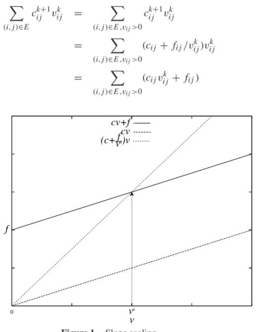
(vk,xk)in (FCNFP), as shown in Figure 1.
(i,j)∈E
cki j+1vi jk =
(i,j)∈E,vi j>0
ci jk+1vki j
=
(i,j)∈E,vi j>0
(ci j+ fi j/vi jk)vi jk
=
(i,j)∈E,vi j>0
(ci jvi jk + fi j) (27)
f
0 vk
v cv+f
cv (c+ fvk)v
Figure 1–Slope scaling.
The linear approximation method is applied to solve (LPC-installation). Here, we fix allxi j =
1, (i,j)∈ A, and solve the next problem (LPC-installation-slope) in which the cost in the objec-tive function is adjusted.
(LPC-installation-slope): min (i,j)∈A
βi jkyi j
subject to (14), (15),i ∈ ¯V \ {N0} (16), (17)
(18), (19),i ∈V+, (i,j)∈ A
(20), (21),i ∈V−, (i,j)∈ A
(9), (i,j)∈ A
(22),i ∈V
(23), (i,j),∈ E
Figure 2 shows the method by which LPC installation problem is solved. The advantage of this method is that a feasible solution is always obtained. As there is no variable representing the in-stallation location, a search for the location is not conducted. By approximating the cost function dynamically, the same cost as the conventional location cost is obtained. It is difficult to prove the convergence of the algorithm theoretically. According to Kim & Pardalos (1999, 2000), this algorithm is a quite efficient heuristic approach for solving concave piecewise linear network flow problems. The numerical experiments show its performance is very stable.
Figure 2–Algorithm for LPC installation.
• Step 0. (Initial setting):We take the number of iterationsk=0,βk=β.ǫ >0 is given.
• Step 1. (Final decision condition):Ifk≥1, then we halt when
(i,j)∈A(yki j−yki j−1) < ǫ. The solutionyki jfinally obtained, is the LPC capacity, whenyi jk > 0,xi j =1 and in all other
casesxi j =0, the solution for (LPC-installation) is obtained.
• Step 2. (Calculation of (FCNFP-LP)):Problem (LPC-installation-slope)is solved, the solu-tiony= ykis obtained.
• Step 3. (Update costs):
βi jk+1 =
βi j+αi j/yi jk ifyki j>0
βi jk ifyki j=0
• Step 4. (Update number of iterations):Letk=k+1 and return to Step 1.
4 NUMERICAL EXAMPLE USING A FULL-SCALE MODEL SYSTEM
4.1 Comparison between local search and the linear approximation method
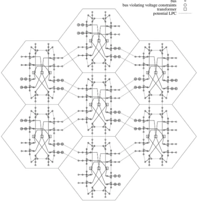
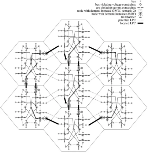
We used a full-system-scale model of a power distribution system to demonstrate the applicability of this method to the optimization of the installation location and capacity. Figure 3 shows the model used, representing a 6.6 kV system supplying power from distribution substations at seven locations, for a standard demand scale of 250 MW per single secondary substation (154/66 kV). We assumed an urban neighborhood with an approximate area of 15 km×15 km, based on the impedance value set at each feeder. The following conditions are used to model the 6.6 kV feeder structure and load.
• One distribution substation has a three-bank (20MVA*3) structure, with four feeders com-ing from each transformer bank.
• There is no supply from the same transformer bank into adjacent feeders.
• It is possible to loop the end nodes of each feeder (three nodes per feeder) with the adjacent feeder.
• The above feeder structure is common to all seven distribution substations.
Figure 3–Power distribution system.
In the calculation, the initial condition was a violation of the operational constraints arising si-multaneously in multiple nodes at the ends of the feeders due to a voltage increase (number of nodes where violation occurred: 44), because of the interconnection of the distributed power sources. This initial condition was used to determine the optimal installation location and capac-ity of the LPC. Simulations were then carried out using the numerical optimizer NUOPT on a 2.00 GHz Xeon E5507 with two processorsand 12.0 GB memory. Examples of modern portfolio optimization problems were given by Scherer & Martin (2005).
This reduction in searching is because there is no requirement to search the 0−1 variable relating to the installation when using the linear approximation method. Linear approximation is a tech-nique that lacks global convergence, and it is not necessary to converge on an optimal solution. In our simulation, the same solution was obtained when using local search and linear approxi-mation, in both cases a suitable solution was obtained for the positional relation with constraint violations in the system.
Although the efficiency of the local search method can be improved by using a set in which the variables representing the installation descision are fixed, the calculation time remains much longer than that of the linear approximation method.
Table 1–Calculation results (local search).
Iterations Number Cost Number of times
of LPCs OPF solved
0 15 17.78 2
1 14 16.92 20
2 13 15.99 20
3 12 15.13 12
4 11 13.75 16
5 11 13.75 14
Total number of times OPF solved 84
Calculation time 15070 (sec)
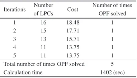
Table 2–Calculation results (linear approximation).
Iterations Number Cost Number of times
of LPCs OPF solved
1 16 18.48 1
2 15 17.71 1
3 13 15.71 1
4 11 13.75 1
5 11 13.75 1
Total number of times OPF solved 5
Calculation time 1402 (sec)
4.2 Investigation of multi-scenario optimization
condition of voltage constraint violations arising in multiple nodes at the ends of feeders (number of nodes where violation occurred: 40). This was due to an increase in demand, with violations of the line thermal capacity constraint arising concurrently in 10 lines. First, we determined the optimal location for the LPC in each individual scenario.
Table 3–Calculation results (per scenario).
Scenario Solution method Calculation Number of time(s) OPF times
1 local search 4997 48
2 linear approximation 391 4
1 local search 3667 70
2 linear approximation 385 4
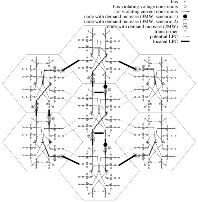
As can be seen from Table 3, the calculation time when using the linear approximation method was much shorter than that of the local search method. The optimal solutions obtained are shown in Figures 4 and 5.
Figure 5–Optimal location (scenario 2).
Next, we consider a model that takes multiple scenarios simultaneously into account. In this model, the variablesx andy are defined as deterministic variables and the variableseand f are defined as stochastic variables representing voltage values. The variableseand f have the subscriptsfor the scenario s, and it can vary for each scenario. The stochastic multi-scenario problem we consider is an extension problem of the original problem (LPC-installation), and it is defined so that the constraints are satisfied for all scenarios. Figure 6 shows the optimal locations when both scenarios were considered.
Figure 6–Optimal location (multi-scenario).
5 CONCLUSIONS
When adressing the LPC optimal installation problem, conventional methods require repeated calculations to be performed both when searching for an installation location and for caluculat-ing the OPF. These approaches require long computational time to produce a solution and make it difficult to perform optimization under multi-scenario constraints. In the present study, we de-veloped a more efficient approach for solving practical problems. Using a technique that linearly approximates the installation cost, it becomes possible to obtain solutions through nonlinear op-timization of the minimum conditions.
This increases the speed of the process. We investigated the effectiveness of our novel technique using a full-scale system model, and demonstrated its capacity to minimize the cost of resolving all voltage violations efficiently, and with a shorter calculation time than conventional techniques based on local searches.
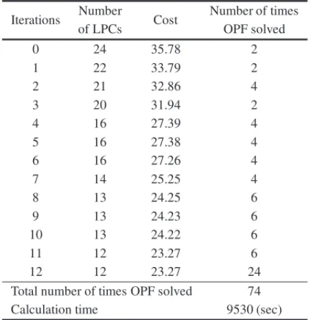
Table 4–Calculation results with multiple scenarios (local search).
Iterations Number Cost Number of times
of LPCs OPF solved
0 24 35.78 2
1 22 33.79 2
2 21 32.86 4
3 20 31.94 2
4 16 27.39 4
5 16 27.38 4
6 16 27.26 4
7 14 25.25 4
8 13 24.25 6
9 13 24.23 6
10 13 24.22 6
11 12 23.27 6
12 12 23.27 24
Total number of times OPF solved 74
Calculation time 9530 (sec)
Table 5–Calculation results with multiple scenarios (slope scaling).
Iterations Number Cost Number of times
of LPCs OPF solved
1 24 35.70 1
2 20 31.79 1
3 16 27.37 1
4 13 24.30 1
5 13 24.27 1
6 12 23.27 1
Total number of times OPF solved 6
Calculation time 886 (sec)
REFERENCES
[1] BAIX, WEIH, FUJISAWAK & WANGY. 2008. Semidefinite programming for optimal power flow problems.Electrical Power and Energy Systems,30: 383–392.
[2] BAZARAAMS, SHERALI HF & SHETTYCM. 1993.Nonlinear Programming-Theory and Algo-rithm, second edition, John Wiley & Sons, New York.
[3] KIMD & PARDALOSPM. 1999. A solution approach to the fixed charge network flow problem using a dynamic slope scaling procedure.Operations Research Letters,24: 195–203.
[5] KIMD & PARDALOSPM. 2000. A dynamic domain contraction algorithm for nonconvex piecewise linear network flow problems.Journal of Global Optimization,17: 225–234.
[6] MOLZAHNDK, HOLZERJT, LESIEUTREBC, DEMARCOCL. 2013. Implementation of a Large-Scale Optimal Power Flow Solver Based on Semidefinite Programming.IEEE Transactions on Power Systems,28: 3987–3998.
[7] RUSZCZYNSKI´ A & SHAPIROA. 2003. Stochastic Programming (Handbooks in Operations Re-search and Management Science, 10), Elsevier.
[8] SCHERERB & MARTIND. 2005.Modern Portfolio Optimization with NUOPTTM, S-PLUSR, and S+BayesTM, Springer.
[9] SHAPIRO A, DENTCHEVAD & RUSZCZYNSKI´ A. 2009. Lectures on Stochastic Programming: Modeling and Theory, SIAM.
[10] SHIINAT. 1999. Numerical solution technique for joint chance-constrained programming problem – An application to electric power capacity expansion.Journal of the Operations Research Society of Japan,42(2): 128–140.
[11] SHIINAT & BIRGEJR. 2003. Multistage stochastic programming model for electric power capacity expansion problem.Japan Journal of Industrial and Applied Mathematics,20(3): 379–397
[12] SHIINAT & BIRGEJR. 2004. Stochastic unit commitment problem.International Transactions in Operational Research,11(1): 19–32.
[13] SHIINAT & WATANABEI. 2004. Lagrangian relaxation method for price-based unit commitment problem.Engineering Optimization,36(6): 705–719.
[14] WOODAJ & WOLLENBERGBJ. 1996. Power Generation. Operation and Control, John Wiley & Sons, New York.