Sequential Protocols’ Behaviour Analysis

(1)

Ricardo Miguel Nunes Camacho de Matos

Licenciado em Ciências da Engenharia Electrotécnica e de

Computadores

Sequential Protocols’ Behaviour Analysis

Dissertação para obtenção do Grau de Mestre em Engenharia Electrotécnica e de Computadores

(2)

(3)

Sequential Protocols’ Behaviour Analysis

The Faculty of Sciences and Technology and the NOVA University Lisbon have the right, perpetual and without geographical boundaries, to file and publish this dissertation through printed copies reproduced on paper or on digital form, or by any other means known or that may be invented, and to disseminate through scientific repositories and admit its copying and distribution for non-commercial, educational or research purposes, as long as credit is given to the author and editor.

Este documento foi gerado utilizando o processador (pdf)LA_{TEX, com base no template “novathesis” [1] desenvolvido no Dep. Informática da FCT-NOVA [2].}

(4)

(5)

(6)

(7)

A c k n o w l e d g e m e n t s

Começo por agradecer ao meu orientador, professor Rodolfo Oliveira por todo o tempo disponibilizado no meu acompanhamento ao longo deste trabalho, mesmo por vezes so-brecarregado, sempre se disponibilizou para qualquer esclarecimento, sem quaisquer restrições e a qualquer hora, tendo sido quem mais impulsionou a conclusão desta disser-tação.

Seguidamente, gostaria de agradecer à FCT-UNL e ao DEE pelas condições proporcionadas que me permitiram desenvolver as capacidades necessárias para poder concluir os meus estudos de forma a me tornar num bom profissional. Também agradeço ao Instituto de Telecomunicações que apoiou o desenvolvimento do trabalho através dos projectos UID/EEA/50008 /2013 e CoShare (com referência LISBOA-01 -0145 -FEDER-030709). Quero ainda agradecer aos meus pais e aos meus avós, por me terem proporcionado todas as condições necessárias para concluir esta etapa tão importante da minha vida. Garanti-ram sempre que nunca nada me faltasse, apoiando-me sempre incondicionalmente nas minhas decisões e por isso um obrigado muito especial por tudo. À minha irmã quero agradecer por toda a paciência e apoio que me tem fornecido ao longo deste tempo, as-sim como à minha namorada por toda a motivação, amor e carinho prestado ao longo desta caminhada. Aos meus restantes familiares mais próximos, por estarem presentes na minha vida e me apoiarem também neste meu trajeto.

(8)

(9)

A b s t r a c t

The growing adoption of the Session Initiation Protocol (SIP) has motivated the devel-opment of tools capable of detecting valid SIP dialogues, in order to potentially identify behavioural traits of the protocol. This thesis serves as a starting point for characterising SIP dialogues, in terms of distinct signalling sequences, and providing a reliable classifi-cation of SIP sequences. We start by analysing sequential pattern mining algorithms in an oﬀ-line manner, providing valuable statistical information regarding the SIP sequences.

In this analysis some classical Sequential Pattern Mining algorithms are evaluated, to gather insights on resource consumption and computation time. The results of the analy-sis lead to the identification of every possible combinations of a given SIP sequence in a fast manner.

In the second stage of this work we study diﬀerent stochastic tools to classify the SIP

dialogues according to the observed SIP messages. Deviations to previously observed SIP dialogues are also identified. Some experimental results are presented, which adopt the Hidden Markov Model jointly used with the Viterbi algorithm to classify multiple SIP messages that are observed sequentially. The experimental tests include a stochastic dynamic evaluation, and the assessment of the stochastic similarity. The goal of these tests is to show the reliability and robustness of the algorithms adopted to classify the incoming SIP sequences, and thus characterizing the SIP dialogues.

(10)

(11)

R e s u m o

A crescente adoção do Protocolo de Iniciação de Sessão (SIP) motivou o desenvolvimento de ferramentas capazes de detetar diálogos válidos de SIP, com o propósito de identi-ficar características comportamentais do protocolo. Esta tese serve como ponto de par-tida para caracterizar os diálogos SIP, em termos de sequências de sinalização distintas e fornecendo uma classificação fidedigna das sequências SIP. Começamos por analisar algoritmos de identificação de padrões sequenciais de uma maneira oﬀ-line, os quais

pos-sibilitam a obtenção de informações estatísticas sobre as sequências SIP. Nesta análise, alguns algoritmos clássicos de Identificação de Padrões Sequenciais são avaliados para obter informações sobre o consumo de recursos e o tempo de computação. Os resultados da análise levam à identificação de todas as combinações possíveis de uma determinada sequência SIP de uma maneira rápida.

Na segunda etapa deste trabalho estudam-se diferentes ferramentas estocásticas para classificar os diálogos SIP de acordo com as mensagens SIP observadas. Também são identificados desvios aos diálogos SIP previamente observados. São apresentados alguns resultados experimentais, os quais adotam o Hidden Markov Model usado conjuntamente com o algoritmo Viterbi para classificar múltiplas mensagens SIP que são observadas se-quencialmente. Os testes experimentais incluem uma avaliação dinâmica estocástica e a avaliação da similaridade estocástica. O objetivo destes testes é mostrar a fiabilidade e robustez dos algoritmos adotados para classificar as sequências SIP de entrada e, assim, caracterizar os diálogos SIP.

(12)

(13)

C o n t e n t s

List of Figures xvii

List of Tables xix

Listings xxi

1 Introduction 1

1.1 Motivation . . . 1

1.1.1 Objectives and Contributions . . . 3

1.2 Thesis Structure . . . 3

2 Related Work 5 2.1 Introduction . . . 5

2.1.1 Types of Data . . . 6

2.1.2 Types of Mining . . . 7

2.2 Introduction to Sequential Pattern Mining . . . 9

2.2.1 Problem definition . . . 9

2.2.2 Taxonomy . . . 11

2.2.3 Structure definition . . . 14

2.2.4 Architectures . . . 15

2.3 Sequential Pattern Mining Algorithms . . . 16

2.3.1 GSP . . . 16

2.3.2 SPADE . . . 19

2.3.3 PrefixSpan . . . 20

2.4 Conclusions . . . 22

3 Off_{-line Evaluation of Mining Algorithms} ₂₅ 3.1 Introduction . . . 25

3.2 SIP Anomaly Detection . . . 25

3.3 System Description . . . 26

3.3.1 Experimental Testbed. . . 26

3.3.2 Data Acquisition and Preparation . . . 27

(14)

CO N T E N T S

3.4 Performance Evaluation. . . 29

3.4.1 Long sequence . . . 29

3.4.2 Short sequence . . . 30

3.5 Final Remarks . . . 31

4 SIP’s Behaviour Stochastic Model 33 4.1 Markov Chains. . . 33

4.2 Hidden Markov Model . . . 35

4.3 Solution: Viterbi Approach . . . 37

4.4 Data Acquisition and Preparation . . . 39

4.4.1 Pre-Processing Step . . . 40

4.4.2 Post-Processing Step . . . 41

5 Experimental Results 45 5.1 Stochastic Dynamics Evaluation . . . 45

5.2 Stochastic Similarity Evaluation . . . 47

5.3 Final Remarks . . . 49

6 Conclusions 51 6.1 Final Remarks . . . 51

6.2 Future Work . . . 52

Bibliography 53 A SIP Dialogue Diagrams 57 A.1 Dialogue 1 . . . 57

A.2 Dialogue 2 . . . 58

A.3 Dialogue 3 . . . 59

A.4 Dialogue 4 . . . 60

A.5 Dialogue 5 . . . 61

A.6 Dialogue 6 . . . 61

A.7 Dialogue 7 . . . 62

A.8 Dialogue 8 . . . 63

A.9 Dialogue 9 . . . 63

A.10 Dialogue 10 . . . 64

A.11 Dialogue 11 . . . 64

A.12 Dialogue 12 . . . 65

A.13 Dialogue 13 . . . 65

A.14 Dialogue 14 . . . 66

A.15 Dialogue 15 . . . 66

(15)

CO N T E N T S

B.2 Provisional Responses. . . 68

B.3 Successful Responses . . . 68

B.4 Redirection Responses . . . 68

B.5 Client Failure Responses . . . 68

B.6 Server Failure Responses . . . 70

B.7 Global Failure Responses . . . 71

C Matlab Scripts 73 C.1 run.m Script . . . 73

C.2 generateSamples.m Script . . . 76

C.3 classification.m Script . . . 76

C.4 saveSequence.m Script . . . 76

C.5 findSequence.m Script . . . 77

C.6 normalizeByRows.m Script . . . 77

C.7 forward_viterbi.m Script . . . 78

(16)

(17)

L i s t o f F i g u r e s

2.1 Sequential pattern mining Architecture . . . 16

3.1 SIP Experimental Testbed. . . 27

3.2 SIPp Custom Dialogues. . . 27

3.3 Long sequence performance analysis . . . 30

3.4 Short sequence performance analysis.. . . 31

4.1 Markov Chain for SIP dialogues.. . . 34

4.2 Hidden Markov Model for relating SIP messages received to the known Dia-logues. . . 36

4.3 The Viterbi trellis. . . 37

4.4 Matlab Viterbi Implementation Scheme. . . 42

5.1 SIP Dynamic Evaluation. . . 46

5.2 SIP Similarity Evaluation. . . 49

A.1 Dialogue 1 (Successful INVITE request). . . 57

A.2 Dialogue 2 (INVITE: 200 OK lost). . . 58

A.3 Dialogue 3 (INVITE: ACK wrong cseq). . . 59

A.4 Dialogue 4 (INVITE: CANCEL after 100 Trying). . . 60

A.5 Dialogue 5 (Successful REGISTER request). . . 61

A.6 Dialogue 6 (REGISTER: 403 Forbidden). . . 61

A.7 Dialogue 7 (UAC Digest Leak). . . 62

A.8 Dialogue 8 (Bad Message). . . 63

A.9 Dialogue 9 (INVITE: 404 Not Found).. . . 63

A.10 Dialogue 10 (INVITE: 503 Service Unavailable). . . 64

A.11 Dialogue 11 (OPTIONS). . . 64

A.12 Dialogue 12 (OPTIONS: 404 Not Found). . . 65

A.13 Dialogue 13 (INVITE: wrong Call ID in bye). . . 65

A.14 Dialogue 14 (SUBSCRIBER). . . 66

(18)

(19)

L i s t o f Ta b l e s

2.1 Sequential database.. . . 10

2.2 Candidate Generation Example. . . 18

2.3 Vertical database. . . 19

2.4 Vertical to Horizontal database. . . 19

2.5 PrefixSpan database examples . . . 21

2.6 S-Matrix . . . 21

3.1 SIP message alphabet.. . . 28

5.1 Known Sequences. . . 46

5.2 Sequence Mapping. . . 47

5.3 Similarity Test Database. . . 48

(20)

(21)

L i s t i n g s

4.1 Viterbi Pseudo-code . . . 38

C.1 run.m script . . . 73

C.2 generateSamples.m script. . . 76

C.3 classification.m script . . . 76

C.4 saveSequence.m script . . . 76

C.5 findSequence.m script. . . 77

C.6 normalizeByRows.m script . . . 77

(22)

(23)

C

h

a

p

t

e

r

1

I n t r o d u c t i o n

Over recent years the need to extract and organize information has become essential, and has been heavily demanded in today’s market. With the increasing number of smart devices that can communicate with each other, the size of databases has increased expo-nentially and the amount of information to process and analyse has simply become too much to handle.

Keeping in mind the amount of time spent analysing information and the performance of the available resources, data-mining has gained an important role in data analysis, with a plethora of algorithms capable of running these tasks autonomously .

In telecommunications the problem of data gathering and analysis has also become rel-evant. The amount of data and signalling transmitted between diﬀerent protocols in

a given period of time can be hard to analyse and, more importantly, hard to identify patterns that could be relevant to better understand the current operational conditions. Consequently, there is a need to find a reliable approach to analyse the behaviours of diﬀerent protocols and take conclusions about the obtained results from the data that is

available.

1.1 Motivation

(24)

C H A P T E R 1 . I N T R O D U C T I O N

of this protocol is associated with the need of implementing analytical tools capable of analysing SIP signalling messages. The goal is to predict the behaviour of the SIP protocol, having the intent of detecting anomalies in the communication sessions. The motivations take into account three major cornerstones:

• Technical Diagnosis: With the rise in the volume of data, the time used in diagnosis has become too extensive, consuming many people and resources in order to fulfil a specific analysis. The goal here is to make diagnosis faster and more accurate, making problem resolution simpler. For instance, in a specific network if packet drop rate increases we want to know what caused the increase as quickly as possible in order to solve the problem before it escalates into something more serious. Big Data algorithms can have an important role in selecting important data, since it can label sets of data into diﬀerent groups, therefore making it easier to analyse

in detail each of these individual sets, and can give additional information that otherwise could be inaccessible in naked eye.

• Planning: Given that observing a series of raw data can be very complex and time consuming, predicting what will happen in the future to the system according with the known data may be even more complicated. This thesis aims to aid in the decision making of plans and procedures in order to identify in an early stage what is happening in the system and if that behaviour will later aﬀ_{ect the performance or}

damage the system as a whole. This may be useful in multiple scenarios. Imagine several packet drops are observed, and by analysing the pattern of the messages it is concluded that if the system keeps going on that direction it will eventually crash, within a week. With the aid of a data mining analysis it is possible to take additional decisions to avoid the crash. This can be achieved by planning the system with parameters that will directly aﬀect the future outcome, therefore preventing

the crash.

• Security: This thesis also intends to improve the security of a given system and prevent external intrusion to information that it may store in a database. This is accomplished again by analysing the behaviour of the system, and finding relations in the patterns that are extracted. If we get a frequent pattern that is deviating from the normal behaviour of the system, we can conclude that something is wrong and that an attack may be in course and it is needed to act on it. By making this verification we are ensuring the integrity and security of our system.

(25)

1 . 2 . T H E S I S S T R U C T U R E

1.1.1 Objectives and Contributions

This subsection describes the objectives that were defined for this thesis as well as a few contributions of this work.

Objectives:

• Elaborate a bibliographic survey on diﬀerent algorithms that are able to categorize

large amounts of data, and extract useful information and knowledge from them. The goal here is to study which algorithms can be used to classify a series of raw data, so the analysis becomes simpler, by extracting information in form of patterns that can predict the behaviour of the system.

• Propose a data categorization framework with low computational complexity, in order to process faster.

• Be eﬃcient and accurate in categorizing the data. To do so will require an extensive

analysis on the selected algorithms for the pattern extraction to identify the most eﬃ_{cient ones and use only those which ensure better results.}

• Apply classic algorithms to innovative scenarios in telecommunications. Here the algorithms chosen that meet the above requirements will be applied to analyse telecommunications Protocol Behaviours. To do so requires the utilization of se-quential pattern mining algorithms and try to incorporate their functionalities and use them in the data selected from message logs provided by these protocols.

Expected Contributions:

• Implement diﬀerent sequential pattern mining algorithms in the context of

com-puter networks. These algorithms will be used to find frequent patterns in telecom-munications protocols, such as SIP and GSM signalling.

• Classify protocol behaviours as ’normal’ behaviours or as ’deviations’ from their normal state. The behaviour analysis can have many diﬀerent applications such as

protocol’s security, by analysing how a certain protocol is expected to behave, or anomaly detection.

• Identify in real time when a deviation of behaviour occurs, always with the aim of understanding why it happened in the first place and where to act to correct it.

1.2 Thesis Structure

(26)

C H A P T E R 1 . I N T R O D U C T I O N

the performance results obtained with diﬀerent sequential pattern mining algorithms.

(27)

C

h

a

p

t

e

r

2

R e l a t e d Wo r k

2.1 Introduction

Sequential pattern mining(SPM) was first introduced by Agrawal and Srikant [1]. In order to understand how this technique works lets start by showing a practical example. Assuming the 4 sequences: <(ab)>, <(abc)>, <(abc)d> and <(abc)dc>, the goal is to dis-cover which of these sequences (or their subsets) are frequent. To accomplish this, it is necessary to determine the frequency with which items belong to each sequence. A min-imum frequency, refered to as minmin-imum support, is usually considered. Looking again at the sequences, and assuming a minimum support of 3, we can classify the sequence <(abc)> as frequent since it appears three times, in <(abc)>, <(abc)d> and <(abc)dc>.

The same can be said of <(ab)>, which is present in all four sequences. On the other hand, considering the sequence <(abc)d>, we observe that it reaches the minimum support threshold, since it does not verify the minimum support equal to 3, appearing only in the last two sequences.

In a more formal way, sequential pattern mining is defined by several other authors [22][30] as a data-mining technique that discovers sequences of frequent item-sets. These sequences can be seen as specific patterns in a sequence database, and the goal of se-quential pattern mining is to extract those sese-quential patterns whose support exceeds a pre-defined minimum support. All the items in one item-set must have the same time stamp or happen within a certain pre-defined window of time in order to be associated to a sequence. A typical example of a sequential pattern is “Customers who buy a digital camera are likely to buy a color printer within a month”.

(28)

C H A P T E R 2 . R E L AT E D WO R K

vast range of applications, such as customer purchase patterning analysis, correlation analysis, and software bug tracking or in the case we present in this thesis, protocol be-haviour analysis. To better introduce SPM we first need to learn some core concepts of this data-mining technique.

2.1.1 Types of Data

There are many types of data that can be mined with mining techniques. Because diﬀ

er-ent data is available, the knowledge extracted will also be diﬀ_{erent, which is very useful}

to take diﬀerent conclusions about the problem we are trying to understand.

Essentially we can categorize data into two diﬀerent types: _Qualitative, and

Quantita-tive. In qualitative type data information is characterized by a symbolic value, because their attributes cannot be measured. An example of qualitative data are colors. If we want to describe a color we can define it as a code (e.g. Black #000000). By doing this, we are transforming colors into categorical variables, where we assign a number that without a context has no meaning at all, but grouped in the category of numbers we can understand what they mean. However, in this type of data it does not make sense to determine a sum of colors or an average, since it has no meaning.

On the other hand, quantitative data can be quantified and verified, being used in sta-tistical manipulation. An example of such data can be seen looking at the example of a shopping cart, where we can define the price of the items and apply arithmetic. In short we can say that quantitative data defines, whereas qualitative data describes. With that in mind we can classify data-mining in diﬀerent categories acording to the data they are

applied to as defined in [30].

• Relational database– Here data is described by a set of attributes which are stored in tables, being a highly structured data repository. Data mining in these relational databases focuses mainly on discovering patterns and trends, being used in banks and in supermarkets to acquire customer behavioural information, such as customer spending habits, and profiling clients into categories such as high and low spenders.

• Transactional database– Refers to a collection of transactions (e.g. sale records), where data-mining enters to find a correlation between items and transaction records. These types of databases have gained popularity due to the increase in e-commerce, with a fast growing community of people that start to make all of their shopping online.

(29)

2 . 1 . I N T R O D U C T I O N

• Temporal and time-series database– For each temporal data item, the correspond-ing time is associated. Can extract more useful information from an individual, by analysing it’s temporal behaviour.

Looking at the problem that this thesis aims to solve, we can define our initial database as atime-series, since in telecommunications when a protocol is running the packets sent and received by a terminal are logged into several files across the network with all the important meta data associated to that instance such as ID, type of message, source, des-tination and finally a time-stamp.

Time stamp is an important attribute to any dataset and, consequentially, important to data mining since it can add more knowledge to the process of extracting informa-tion. For that reason, sequential pattern mining has an important role in these types of databases, since it is used to find the relationships between occurrences of sequential events, although it is used in a special case of time series databases known as Sequential databases that can come whit or without a concrete notion of time.

2.1.2 Types of Mining

In the context of data mining it is possible to identify several types of mining, each of which applies diﬀerent techniques to the data, extracting distinct knowledge. Data

min-ing can be classified into two separate classes acordmin-ing to the data they are applied to, defined in [30] as: descriptive mining that has the goal to summarize general properties of data, and prescriptive data that performs inference on current data to make predictions of what will come next.

Given these two classes of data mining we can identify several techniques, reported with a few examples.

Association Rules– First introduced in [3], an association rule aims to extract interest-ing correlations, frequent patterns and associations between sets of items in a database. In a more formal explanation letL =I1, I2, ..., In be a set of items. An association rule means a relationship of the formX=> Ij, beingXsome set of items fromLandIj a single item not belonging toX. The rule is satisfied if for a confidence factor 0<c<1 at least c% of the transactions in a database satisfy bothX andIj.

(30)

Classification - Described in Han and Kamber (2000)[15], the objective of this tech-nique is to automatically build a model that can classify a class of objects, in order to predict the classification of future objects. Data classification can be seen as a two-step process.

In the first step, a classifier is built to describe a set of predetermined data classes, be-ing called thelearning step. Here a learning algorithm is used to build the classifier by analysing a set of data calledtraining set. In this collection of training data, the classes and concepts that they belong to are predefined and provided so we can also define this step assupervised learning. The final step is used to test the classification accuracy by using the model to classify other test examples. Since the classifiers tend to overfit the data, atest setis used to be classified by the model. The final accuracy will depend on the percentage of accurate classifications the model does to the test set.

An example of a classifier could be a model to categorize bank loan applications assafe orrisky, or catalogue a car asSports carorFamily van.

Clustering - Contrary to the classification method, clustering uses an unsupervised learning process, which means that there are no predefined classes to the initial data set (training set) which is very common in large databases, because assigning classes to every single object can become quite costly. As defined by Han and Kamber (2000) [15] clustering is the process of grouping a set of physical or abstract objects (data) into classes of similar objects also known asclusters. Objects within a same cluster have high similarity, but are very dissimilar to objects in other clusters. Similaritiesare defined by functions, usually quantitatively specified as distances or other measures defined by domain experts.

Clustering applications are manly used in market segmentation, that categorize cus-tomers into diﬀerent groups so that organizations can provide personalized services to

each group.

Regression analysis - This method is the most widley used aproach fornumeric pre-diction, which is the the task of predicting continuous (or ordered) values for a given input [15]. Regression involves learning a function that maps a data item to a real-valued prediction variable [10], and can be used to model the relationship between one or more independent/predictorvariables and adependent/responsevariable. In the context of data mining, the predictor variables are the attributes of interest describing the tuple (i.e., mak-ing up the attribute vector). Generally, the values of the predictor variables are known, being the response variables predicted by these methods.

(31)

2 . 2 . I N T R O D U C T I O N TO S E Q U E N T I A L PAT T E R N M I N I N G

such as Poisson regression, log-linear models and non-linear regression, although most of the problems can be solved simply by using linear regression.

Summarization - Consists in methods used to find a compact description for a sub-set of data[10]. This type of techniques are often used in interactive exploratory data analysis and automated report generation. Data summarization is very important in data preprocessing and is used for measuring the central tendency of data (e.g. mean, median and mode), measuring the dispersion of data (e.g. range, variance and standard devia-tion) and graphical representations such as histograms and scatter-plots are also useful to facilitate the visual inspection of the data [15].

Anomaly detection- This method builds models of normal network behaviour defined asprofileswhich are then used to detect the presence of new patterns that significantly de-viate from the generated profiles [15]. These deviations may represent actual intrusions in the system or simply new behaviours that are not included in the profile. The advan-tage of this technique stands on the fact that it can detect novel intrusions that have not yet been observed, a human analyst needs to sort through all the deviations to ascertain which ones are real intrusions. A limitation of this method is the high percentage of false positives, which can be somewhat corrected by adding the new behaviours of the system to the profile. The new patterns of intrusion can be added to the set of signatures for misuse detection.

All these mining techniques are still used until this day and remain eﬀective

depend-ing on the paradigm they are inserted into, havdepend-ing many research papers dedicated to study each of these techniques in detail [30]. The next section of this chapter will bring more light to the case in study in this thesis, sequential pattern mining.

2.2 Introduction to Sequential Pattern Mining

2.2.1 Problem definition

This section defines the problem of mining sequential patterns, and also give some in-sights on the concepts used in this area. The basis for this definition was taken from [22], and can be viewed as follows. Given:

(i) A set of sequential records (sequences) representing a sequential databaseD.

(ii) A minimum support threshold.

(iii) A set ofkunique events or itemsI=i1,i2, . . . ,ik.

(32)

support), in order to describe the data or predict future data. In order to better under-stand this problem we introduce diﬀerent definitions that represent the roots of diﬀerent

techniques capable of mining sequential patterns.

Definition 1 Let I = I1, I2, I3, ..., In be the set of allitems. Aitem-setcan be viewed as a non-empty, unordered collection of items.

The item-set is denoted (xl x2... xq), where xk is an item. The brackets are omitted if an item-set has only one item, that is, (x) is written simply as x. An example of an item-set can be seen in a grocery store, where the items can be represented by a list of products bought at the same time such as bread, milk and cheese, represented by (abc). Note that the items all belong in the same event since they were all bought at the same transactional time.

Definition 2 Asequenceis a lexicographically ordered list of item-sets (events), such as S = <e1e2e3... el> where the order of the item-sets has an important role, in this case e1occurs

before e2, which occurs before e3, and so on. The event ej is also called an element of S [15].

Let S be represented by <(ab)b(bc)c(cd)>. An item can occur only once in a given item-set, but it can have multiple instances in diﬀ_{erent item-sets of a sequence. In sequence S, the}

item b has three instances, appearing in the item-sets (bc), (b) and in (ab). However, if we were to add the item-set (dcd) to the sequence S it would not be possible, since it contains two instances of the same item.

Definition 3 Given a sequenceS, itssupport, denoted asσ(S), can be defined as "The total number of sequences of whichSis a subsequence divided by the total number of sequences in the databaseD", whereas thesupport countof a sequenceSis the total number of sequences inDof whichSis a subsequence.

A sequence can only have the classification offrequentif its support count (frequency) is greater or equal to the user-definedminimum support. An example of what a sequential database may look like is shown in table2.1.

Table 2.1: Sequential database.

Sequence ID Sequence of items

1 <a(abc)(ac)d(cf)>

2 <(ad)c(bc)(ae)>

3 <(ef)(ab)(df)cb>

4 <eg(af)cbc>

(33)

Definition 4 A subsequenceS’ ofSis denoted byS’⊆S. Formally, a sequence a=<a1, a2...an> is a subsequence of b=<b1b2...bm>, and b is a supersequence of a, if there exist integers 1≤

i1< i2< . . . < in≤msuch thata1⊆bi1,a2⊆bi2, . . . ,an⊆bin[4].

Finnally, we can have a formal definition ofSequential pattern, which is a sequence of itemsets that frequently occurred in a specific order. All items in the same itemsets are supposed to have the same transaction-time value or be included within a time gap [30], which will be defined asmax-gap. Observing a client transaction sheet all of its trans-actions can be viewed together as a sequence, where each individual transaction can be represented as an item-set of that sequence, that are ordered in a certain transaction-time.

2.2.2 Taxonomy

This thesis adopts the taxonomy defined in [22], where sequential pattern mining algo-rithms are categorized in three main categories: Apriori-based,Pattern-growthand Early-prunning. This taxonomy is used to classify sequential pattern mining algorithms based on the characteristics that the diﬀ_{erent techniques provide. It also helps to better}

under-stand and distinguish these techniques before-hand, having some previous knowledge of the characteristics and capabilities of a given algorithm, by looking at what category it belongs.

This section gives examples in some of the key characteristics from each of the categories mentioned above. The focus is on the characteristics that are intrinsic to the algorithms, which include, SPADE[29], GSP[26] and PrefixSpan[17].

Apriori-based:Algorithms that fit into this category depend mainly in the apriori prop-erty which states that“All nonempty subsets of a frequent itemset must also be frequent”[22]. Besides that apriori algorithms are also described as being antimonotonicor downward-closed, which means that if a given sequence cannot pass a pre-defined minimum support test, all of its supersequences will also fail the test, and consequently will be discarded as candidates of frequent sequences. There are three key characteristics that are used in apriori-based methods which are discussed bellow:

1. Breadth-first search: This characteristic is used to describe apriori-based algo-rithms because all of thek-sequences are constructed together in eachkth iteration of the algorithm as it travels trough the data. So suppose the goal is to construct the length-3 sequences. In this method, all of the length-2 sequences must be solved first in order to proceed. This makes available a lot of information that can be used in pruning, but comes with a trade-oﬀbetween information availability and

(34)

2. Generate-and-test:Introduced by the Apriori algorithm in [3], uses exhaustive join operators, where the pattern continues growing one item at a time, being always tested against the minimum support to ensure the given sequence is frequent. This causes the generation of an enormous number of candidate sequences, that can consume a lot of memory in the early stages.

3. Multiple scans of the database:As the name suggests, this characteristic is based on scanning the original database every time it needs to ascertain if the generated candidate sequences are frequent. This scanning keeps on going as long as there exists candidate sequences that need to be verified. This method is very costly in terms of processing time and I/O. A solution to this limitation comes with the introduction of the next category.

Pattern-Growth: Algorithms that fit this category usually display better performance than apriori-based, both in processing time and in memory consumption. This method was implemented to serve as a solution to the problem ofgenerate-and-test that was present in the early apriori algorithms. The goal of this technique is to avoid the candi-date generation step altogether, and the search is only done in a restricted portion of the initial database. In order to fulfil the needs of pattern-growth algorithms diﬀ_{erent key}

characteristics must be considered, including:

1. Candidate sequence pruning:Pattern-growth algorithms like PrefixSpan and oth-ers, attempt to use a data structure that allows pruning of candidate sequences in the early stages of mining. Algorithms that do so have a smaller search space, which in return results in a more directed and narrower search procedure. This charac-teristic is also present in early-pruning techniques, that will be discussed later in this section. The diﬀerence is that early-pruning algorithms try to predict future

candidate sequences, in an eﬀ_{ort to avoid generating them in the first place.}

2. Search space partitioning: This characteristic can be seen in some apriori-based algorithms like SPADE, in spite of being a characteristic of pattern-growth. As the name suggests it provides partitioning of the search space generated, being mostly used in large sets of candidate sequences. This characteristic plays an important role in pattern-growth algorithms, since it is used by nearly everyone of them, with the goal to generate as few candidate sequences as possible. This in extent pro-vides an eﬃcient memory management. There are diﬀerent ways to partition the

search space. SPADE represents the search space as alatticestructure which will be discussed in more detail in later sections. Others such as WAP-mine[24] use a tree-projection structure (this algorithm will not be covered in this thesis).

3. Suffi_{x/Prefix growth:}Used in algorithms that are dependent on projected databases

(35)

each frequent item as a prefix or a suﬃx, after that the candidate sequences are built

around these items and are mined recursively. This is done taking in account that frequent subsequences can always be found by growing a frequent prefix/suﬃx.

This characteristic greatly reduces the amount of memory required to store the diﬀerent candidate sequences that share the same prefix/suﬃx.

4. Depth-first traversal:In this case each pattern is constructed separately, in a re-cursive way. All the subsequences are processed at each level before moving on to the next [28]. This characteristic uses less memory and less candidate sequence generation than breath-first search, having in extent a more directed search space. SPAM [5] is an algorithm that relies heavily in this characteristic. SPADE can also employ this method.

Early-Pruning: These types of algorithms are defined as using some sort ofposition in-ductionto prune candidate sequences at a very early stage in mining. This technique used in the LAPIN algorithm as defined in [27], is used during the mining process and checks the items last position to see if it is smaller than the current prefix position. When this condition is verified, the item cannot appear behind the current prefix in the same cus-tomer sequence. By doing this, the support counting is avoided as much as possible and the generation of infrequent candidate sequences is kept at a minimum. Characteristics of this category are as follows:

1. Support counting avoidance: The idea behind this characteristic is to compute support of a candidate sequence without carrying a count throughout the mining process, and thus avoid scanning the sequence database each time it is needed to compute this support. The advantage of this characteristic is the removal of the sequence database from memory once it stores candidate sequences along with their corresponding support count.

2. Vertical projection of the database:This characteristic is also used in the SPADE algorithm [29] needing only to visit the sequence database once or twice, which then proceeds to construct a bitmap or position indication table for each frequent item, thus, obtaining a vertical layout of the database which is represented in tables2.3

and2.4. These tables are used in the mining process to generate candidate sequences and count their support. This characteristic has the advantage of reducing memory consumption, but on the other hand requires quite a lot computational power.

(36)

2.2.3 Structure definition

Being SPM a data-mining technique it has to follow the same structure as any data-mining algorithm would do. The operation cycle of data mining is divided in 3 stages [30]:

• Preprocessing - It is performed before any data-mining techniques are put into work, having the goal of cleaning and selecting the data for use from a raw database.

• Data mining process- At this stage the diﬀerent data mining techniques are used

in order to extract information and knowledge from the selected data.

• Postprocessing- Evaluates the mining result according to the user requirements.

The work-flow of the previously mentioned processes begins with cleaning and integrat-ing the initial databases where we will get our raw data. The need to do so arises from the fact that information may come from several databases with diﬀerent names to define

the same concept, or even in the same database some inconsistencies may be found with missing or duplicate information. Suppose we have a supermarket that needs to check the sales revenue from a certain item in its store and there are lots of brands on sale but all of them have the same base vending item. In this case, we need to group all sales of each brand together in order to have a notion of the big picture and get a general overview of the sales of the item to analyse.

Since not all of the data in the database is related to our mining task, after cleaning and integrating the data, the next step is to select the task related data. Taking the ex-ample of this thesis we shape the information in order to obtain a sequential database, with sequences from telecommunication protocols, which will leave our database not only smaller, but ready to be mined.

The second process involves the use of data mining techniques applied to the selected data in order to extract diﬀerent information or diﬀerent knowledge [30]. The range of

information extracted may vary depending on the adopted algorithm. In the particular case of Sequential pattern mining the knowledge we acquire consists in frequent item-set patterns.

(37)

2.2.4 Architectures

Being Sequential pattern mining a particular case of data mining, we can describe its architecture in a typical data mining system. Data mining can have a broad view in functionality. It is described in [15] as the process of discovering interesting knowledge from large amounts of data stored in databases, data warehouses, or other information repositories. So a typical data mining system can have several components distributed across the diﬀerent processes associated to this technique. Taking into account the

struc-ture defined for SPM we can look at the architecstruc-ture as follows:

• Pre-processing: This step intends to treat the data to be mined, so it starts with aData Repository. This can be either one or a set of databases/other kind of infor-mation repositories where the inforinfor-mation to be analysed is going to be extracted. Usually, the data contained on these repositories may be in a “raw” state, meaning that before extracting information, data cleaning and integration techniques may need to be done. These techniques involve removing any noise or inconsistent data that can be found in the initial repositories, combining distinct data sources into a whole and begin the selection of the pieces of data that are relevant for our mining task.

After the initial “cleanse”, the information extracted comes in the form ofclean data. The data extracted is then transformed to a format that is ready to be mined, by performing diﬀerent techniques such as summary or aggregation operations.

• Data mining process:This step is where the user interacts with the system, by giv-ing the initial parameters to start the sequential pattern mingiv-ing. These parameters can vary from minimal supports, to the selection of the Algorithm used.

• Data Post-processing: After applying the SPM techniques on the selected data, some knowledge will come out of that mining, in the form of frequent sequential patterns. These results are then evaluated, asserting if the outcome is the desired. If the information extracted is insuﬃ_{cient or has no substantial value to the}

prob-lem the system is trying to solve, the data mining process repeats until these final conditions are reached. In the repeating process the user inserted parameters are changed in order to obtain diﬀ_{erent results.}

(38)

Figure 2.1: Sequential pattern mining Architecture

2.3 Sequential Pattern Mining Algorithms

This thesis will cover three of the most popular algorithms in sequential pattern mining, that possess the most bibliography available which will later be used to implement the protocol’s behavioural analysis. The objective of this section is finding the diﬀerences

between each of these implementations. It will include a brief overview of the selected al-gorithms, ending with several evaluation results capable of comparing their performance.

2.3.1 GSP

(39)

2 . 3 . S E Q U E N T I A L PAT T E R N M I N I N G A LG O R I T H M S

each item, which means it counts the number of occurrences of the item in the data-sequences. At the end of this first pass, the algorithm knows which items pass the min-imum support test, and consequently determine which of them are frequent. This pass generates a seed set which represents the frequent sequences found, that are to be used on the next iteration of the algorithm. The seed set is used to generate candidate sequences that have one more item than the seed set, and consequently all candidate sequences will have the same number of items. The support of the candidate sequences is found during the pass over the data, being based on the minimum support. These candidate sequences are tested to determine if they are frequent or not. If they become frequent they will be used as the seed for the next candidate generation. The algorithm only stops when no frequent sequences nor candidate sequences are generated at the end of the pass.

GSP is described as having two sub-processes:

Sequence candidate generation:In this process candidatek-sequences are generated

based on the set of all frequent (k-1)-sequences. First lets introduce the notion of a con-tiguous subsequenceas it is presented in [26].

Definition 5 Given a sequence S = <S1 S2...Sn> and a subsequence C, C is a contiguous subsequence ofSif any of the following conditions hold:

1. C is derived fromS by dropping an item from eitherS1orSn.

2. C is derived fromS by dropping an item from an elementSi which has at least 2 items.

3. C is a contiguous subsequence ofC′, andC′ is a contiguous subsequence ofS.

For example, consider the sequenceS= <(ab)(cd)(e)(f)>. The sequences <(b)(cd)(e)>, <(ab)(c)(e)(f)> and <(c)(e)> are some of the contiguous sequences ofS. However <(ab)(cd)(f)>

and <(a)(e)(f)> are not.

Candidates are generated in two steps, similarly to the candidate generation procedure for finding association rules described in [2].

• Join Phase- here a sequenceS₁joins another sequenceS₂both belonging to the seed setLk, if the subsequence obtained by dropping the first item inS1is the same as

the subsequence formed by dropping the last items inS2. The generated candidate

sequence by joining S₁andS₂ is the sequenceS₁ extended by the last item ofS₂

(40)

• Prunning Phase- those candidate sequences that have a contiguous subsequence whose support count is less than the minimal support (infrequent) are deleted.

An example of this can be seen in Table 2.2. In the join phase, the sequence <(1, 2)(3)> joins with <(2)(3, 4)> to generate <(1, 2)(3, 4)> and with <(2)(3)(5)> to gener-ate <(1,2)(3)(5)>. In other hand the sequence <(1, 2)(4)> does not join with any quence since there is no sequence of the form <(2)(4, x)>. In the prune phase the se-quence <(1,2)(3)(5)> is dropped since there is no support for its contiguous subsese-quence <(1)(3)(5)>.

Table 2.2: Candidate Generation Example.

Frequent sequences After join After prunning

<(1, 2)(3)> <(1, 2)(3, 4)> <(1, 2)(3, 4)> <(1, 2)(4)> <(1, 2)(3)(5)>

<(1)(3, 4)> <(1, 3)(5)> <(2)(3, 4)> <(2)(3)(5)>

Candidate support count: This final sub-process starts by using an adaptation of the hash-tree structure of [2] to reduce the number of candidates to check the support count. After that the Contain Test is introduced to check if a data sequence D contained a

candidate sequenceS, being composed of two phases:

• Forward phase:GSP finds successive elements of the candidate sequenceS in the

data sequenceDas long as the diﬀerence between the end-time of the element just

found and the start-time of the previous element is less than the user defined time constrainmax-gap. If the diﬀerence is more than max-gap, the algorithm switches to

the backward phase. If an element is not found, the data-sequence does not contain

S.

• Backward phase:The algorithm backtracks and “pulls up” previous elements. Sup-pose the current element is represented bySiand the end-time (Si)=t. The algorithm

checks if there exists transactions containingSi-1and their transaction-times are

af-ter t-max-gap. Since afaf-ter pulling upSi-1the diﬀerence betweenSi-1andSi-2may not

(41)

2.3.2 SPADE

SPADE is an algorithm developed by Zaki (2001) [29], and it relies on theLattice The-ory defined in [7]. The goal is to find frequent sequences using eﬃcient lattice search

techniques and simple join operations. All the existing sequences are usually discovered with only two or three passes over the database. Besides that, SPADE utilizes combina-torial properties to decompose the original problem into smaller portions, which can be independently solved in main-memory. The sequential database is transformed into a vertical data format as in the example in Table2.3, where the new database becomes a set of tuples of the form <itemset: (sequence_ID,time_ID)> [18] and each item id is associated with the corresponding sequence and time stamp. An example of the tuples present in the itemset <(a)> are (1,23), (6,6) and (21,2).

Table 2.3: Vertical database.

<(a)> <(b)> <(c)> <(d)> <(e)>

(SID , TID) (SID , TID) (SID , TID) (SID , TID) (SID , TID)

(1 , 23) (2 , 36) (1 , 26) (6 , 12) (6 , 23)

(6 , 6) (7 , 18) (21 , 26)

(21 , 2)

SPADE can be seen as a three step method. Firstly, it scans the vertical database to com-pute frequent 1-sequences in an apriori-like way. For each database item, the id-list is read from the disk to memory, and then the id-list is scanned and the support is incre-mented for each new sequence ID (SID) found.

The next step involves finding the frequent 2-sequences. A vertical-to-horizontal transfor-mation is preformed on the database. For each itemi, its id-list is scanned into memory. We then look for each (SID,TID) pair abbreviated as (s,t). We group those items with the TID (i,t)and order in increase of SID, and the resulting database is shown in table2.4.

Table 2.4: Vertical to Horizontal database.

SID (Item,TID) pair

1 (a,23) (d,26) 2 (a,19) (b,36) 6 (a,6) (e,12) (g,23)

7 (b,18)

21 (a,2) (h,26)

(42)

that the lattice can grow very big and cannot fit in the main memory. In order to solve this problem, Zaki (2001) [29] proposed that the lattice can be decomposed into disjoint subsets calledequivalence classes, by assigning sequences with the same prefix items to the same class. With this partition, each subset can be loaded and searched seperatly in main memory. The lattice is then traversed for support count and enumeration of frequent sequences[22]. There are two methods used to traverse the lattice, which are

breadth-first(BF) anddepth-first(DF) used in the SPAM algorithm [5].

In breadth-first search, the classes are generated in a recursive bottom-up manner [30] (e.g., to generate the 3-item sequences all the 2-item sequences have to be processed). Depth-first search only needs one 2-item sequence and ak-item sequence to generate a

(k+1)-item sequence. Pruning is also applied in this third step, using the apriori property

[2] when intersecting id-lists (temporal joins) and counting support[22]. Comparing the two methods, we can conclude that Depth-first search dramatically reduces computation and the number of id-lists generated, needing less memory. However, breadth-first search has the advantage of having more information to prune candidate k-item sequences.

2.3.3 PrefixSpan

PrefixSpan [17] is based on the general idea of examining only the prefix subsequences and project only their corresponding postfix subsequences into projected databases. In each projected database, sequential patterns are grown by exploring only local frequent patterns. This algorithm employs database projection in order to shorten the database on the next pass, which in return speeds up computation. In this method, there is no need for candidate generation, since it recursively projects the database according to their prefix.

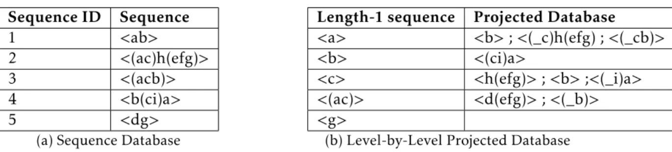
To illustrate the idea of projected databases, consider <a>, <(ac)> and <(ac)h> from the sequential database in Table2.5a. These areprefixesof the sequence <(ac)h(efg)>. On the other hand we can call <(_c)h(efg)> thepostfixof the sequence <a>. An example of a Projected Database, assuming a support count of 2, can be seen in Table2.5b, containing a portion of all the lenght-1 sequences.

There are three diﬀerent projection methods that can be used in PrefixSpan, which are

level-by-level,bi-leveland finallypseudo projection[30]. The first method presented acts in three steps:

1. Scan the sequential database to obtain the length-1 sequences.

2. Divide the search space into diﬀerent partitions, where each partition corresponds

(43)

Table 2.5: PrefixSpan database examples

Sequence ID Sequence

1 <ab>

2 <(ac)h(efg)>

3 <(acb)>

4 <b(ci)a>

5 <dg>

(a) Sequence Database

Length-1 sequence Projected Database

(b) Level-by-Level Projected Database

a prefix (e.g., for the frequent 1-sequence <a> as the prefix the projected database is shown in Table2.5b). The projected database only contains the postifx of these sequences.

3. Find subsets of sequential patterns where these subsets can be mined by construct-ing projected databases, and minconstruct-ing each one recursively. This process is repeated until the projected database is empty or no more frequent length-ksequential pat-terns are generated.

In this method, there is no candidate generation process, although it costs time and space to construct the projected databases.

The next method,bi-levelprojection, relies on the S-Matrix, introduced in [16], and was proposed to reduce the number and size of projected databases. It starts by performing the same first step as the previous method, which is finding all length-1 sequential pat-terns. Assuming the databaseS in Table2.5we have: <a>, <b>, <c>, <(ac)> and <g>.

In the second step a 5x5 lower triangular matrixM is constructed as shown in Table2.6, that represents all the supports for the length-2 sequences, for example M[a,c]=(2,1,2) counts the support for <ac>, <ca> and <(ac)> respectively. Since the information in cell M[c,a] is symmetric to that in M[a,c], a triangle matrix is suﬃ_{cient, this matrix is}

calledS-Matrix[17]. After this the S-Matrix for the frequent length-2 sequences is con-structed, and the process are iterated until no other frequent sequences can be found or the projected database becomes empty. The use of this matrix provides fewer and smaller projected databases.

Table 2.6: S-Matrix

a 0

b (2,1,1) 0

c (2,1,2) (1,1,1) 0

(ac) (0,0,0) (0,1,1) (0,0,0) 0

g (1,0,0) (0,0,0) (1,0,0) (1,0,0) 0

(44)

Pseudo projection is used to make the projection more eﬃcient when the projected

database can be fitted in main memory. In this method, no physical projected database is constructed in memory, instead each postfix (projection) is represented by two pieces of information: pointer to the sequence in the database and oﬀset of the postfix in the

sequence for each size of projection [22].

2.4 Conclusions

This section presents a comparison between the sequential pattern mining algorithms discussed before, focused on the computation time and memory consumption.

GSP is based on the apriori-based category, as it explores a candidate generation-and-test approach [2] to reduce the number of candidates to be examined. However, this technique inherits some costs that are independent of the implementation techniques used [25].

1. Excessive candidate sequence generation.The set of candidate sequences includes all the possible permutation of elements and repetition of items in a sequence, which in turn generates an explosive set of candidate sequences.

2. Multiple scans of the database.The length of a candidate sequence grows by one each time the database is scanned. In a short, to find the sequential pattern with a length oflthe database needs to be scanned at leastltimes.

3. Diffi_{culty in mining long sequential patterns.}A long sequential pattern contains

a combinatorial explosive number of subsequences, and such subsequences must be generated and tested in the a priori-based mining. Thus, the number of candidate sequences is exponential to the length of the sequential patterns to be mined.

The implications of these problems makeapriori-basedalgorithms, such as GSP, compu-tationally expensive due to maintaining the support count for each subsequence being mined, which leads to a huge memory consumption in the early stages of mining. The explosive number of candidate sequences also introduces I/O delay, due to the need to utilize a secondary storage in case the number of sequences gets to big. Despite that, GSP and its predecessorAprioriAll[1] generate all the sequential patterns although being ineﬃ_{cient. They are also the basis of further researches on mining sequential pattern,}

since they first introduced sequential pattern mining.

(45)

2 . 4 . CO N C LU S I O N S

leads to an excessive generation of candidate sequences. However, SPADE finds a solution to this problem by including some Pattern-Growth characteristics such as search-space partitioning, which includes the vertical database layout defined in [28]. This technique reduces scans of the sequence database, making the algorithm faster. Also, the inclusion of lattice structure partitioning allows to load the decomposed search space into main memory to be mined separately. This strategy provides a more eﬃcient memory

manage-ment and minimizes I/O costs [29].

On the other hand, the basic search methodology of this algorithm relies onbreadth-first searchandApriori pruning. Despite the pruning, it has to generate large sets of candidates in breadth-first manner in order to grow longer sequences. Thus, most of the diﬃ_culties

suﬀered in the GSP algorithm occurs in SPADE as well [15]. One way to minimize this

problem is to use adepth-first searchstrategy that requires less memory.

PrefixSpan falls under the Pattern-Growthcategory, and like many other algorithms of this type the key idea for this method is to avoid the candidate-generation step alto-gether, which is the most time consuming part of apriori algorithms such as GSP [30]. It employs the database projection technique to make the database for the next pass much smaller turning the algorithm faster because the search space is reduced at each step (increasing the computation time in the presence of small support thresholds) [4]. This characteristic greatly reduces memory consumption in terms of candidate sequences. The main cost of PrefixSpan lies in the projected database generation process, which can be computationally expensive if the databases have to be generated physically. To solve this problem, pseudo-projection was suggest to replace the physical projection of a sequence by a sequence identifier. However, this method can only be applied if the projected databases can be fitted into main memory. PrefixSpan also outperforms other algorithms if the sequential pattern is very long, since it can handle its treatment more eﬃciently.

(46)

(47)

C

h

a

p

t

e

r

3

O f f - l i n e E va l ua t i o n o f M i n i n g A l g o r i t h m s

3.1 Introduction

This chapter focuses on SIP signalling anomaly detection based on probabilistic hypothe-ses, which may also be adopted to support SIP signalling behaviour prediction, this work is a first step to analyse SIP dialogues in terms of occurrence of signalling patterns.

We start to describe the considered SIP dialogue and the diﬀerent SPM algorithms

capable of identifying similar SIP signalling sequences and their occurrence rate. Af-ter describing how SIP signalling messages are filAf-tered, we evaluate the computation performance of the SPM algorithms for multiple SIP dialogues. The evaluation metrics include the computation time and memory required to identify all SIP sequences and subsequences that form the SIP dialogue. The performance results show that both compu-tation time and memory usage linearly grow with the number of SIP dialogues, allowing the use of the adopted algorithms for high number of SIP dialogues. This conclusion is of particular relevance to future adoption of SPM algorithms in real-time SIP signalling anomaly detection schemes.

This chapter is organized as follows. Section 3.2 identifies related work on SIP anomaly detection. Section 3.3 introduces the SIP architecture adopted in this work. The evaluation of the performance achieved by the SPM algorithms applied to the SIP dialogues is described in Section3.4. Finally, Section3.5concludes the chapter.

3.2 SIP Anomaly Detection

(48)

C H A P T E R 3 . O F F - L I N E E VA LUAT I O N O F M I N I N G A LG O R I T H M S

studied in multiple works, since attacks may be attempted by simply changing the text-based SIP message headers. Malicious SIP messages are usually detected through intru-sion detection systems (e.g. firewalls) [21], learning techniques [23] and/or identification of deviations from a priori statistics [19]. The focus of our work is not on the malformed SIP messages but rather on the identification and characterization of SIP dialogues. In [11] support-vector-machine classifiers were adopted to label incoming SIP messages as goodorbad. A SIP message lexical analysis was developed to filter the messages that are not formed according to the standard and in a second stage a semantic filter was applied to the stream of the surviving messages to remove syntactic errors. The work in [14] models the SIP operation as a discrete event system where the state transitions of the SIP dialog are described through a probabilistic counting deterministic timed automata. The description includes the characterization of the SIP sequences and their timmings, which are used a posteriori to detect deviations from the models. Contrary from [14], in our work we do not assume a fixed probabilistic model of the SIP operation. Instead, we are interested in monitoring the SIP messages to characterize the SIP dialogues through the sequences and subsequences that compose them, as well as their occurrence probability.

3.3 System Description

3.3.1 Experimental Testbed

The data repository used in this work was obtained through the generation of SIP mes-sages considering multiple SIP dialogs. The SIP dialogs were generated with SIPp [13], which is a free Open Source SIP traﬃc generation tool. SIPp allows the creation of

cus-tomized XML dialogues to define which messages are exchanged between the SIP end users, allowing the occurrence of errors in the transmission of the SIP messages.

(49)

3 . 3 . S YS T E M D E S C R I P T I O N

Figure 3.1: SIP Experimental Testbed.

3.3.2 Data Acquisition and Preparation

In the architecture in Figure3.1, SIPp was used to establish SIP dialogues with the Aster-isk Server. The flow of the SIP messages starts from the SIPp Generator, being then routed to the Asterisk server, which analyses the received SIP messages and acts accordingly.

(a) INVITE Request. (b) REGISTER Request.

Figure 3.2: SIPp Custom Dialogues.

To generate traﬃ_{c in the SIP Tra}ﬃ_{c Host a few SIP dialogues were defined}

(50)

C H A P T E R 3 . O F F - L I N E E VA LUAT I O N O F M I N I N G A LG O R I T H M S

generated by the SIPp application, detailing each of the SIP messages sent and received. The logs were then cleaned and converted into a more compact format to be mined by the sequential pattern mining algorithms studied in this work (GSP, SPADE and PrefixSpan). To achieve this goal, the SIPp log files were processed using bash scripting with the intent of isolating each message, whether it is a SIP REQUEST or a SIP RESPONSE, by their type (e.g. INVITE, REGISTER, 200 OK), and by Call-ID. The Call-ID is a globally unique identifier of a SIP call. A set of received and sent SIP messages can contain the same Call-ID, therefore representing a time-ordered sequence of messages that constitute a given SIP dialogue. The aggregation of messages by Call-ID and by type represent the time-ordered SIP sequence to be mined.

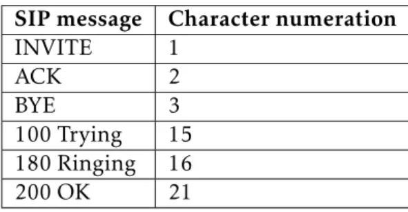
Assuming the dialogue in Figure3.2a, which represents a successful INVITE request, an ordered sequence of events can be defined through the signalling messages exchanged between the client and the server. The session starts by sending an INVITE message, which then waits for the server response. After the acknowledgement by the client origi-nating the invite, the session is established until one of the actors (caller/callee) ask to end the call by sending a BYE message. A possible sequence of SIP messages forming the SIP dialogue can be represented by: <INVITE, 100 Trying, 180 Ringing, 200 OK, ACK, BYE, 200 OK>. This sequence of events represents the INVITE dialogue, which is associated to an unique Call-ID. Adopting a specific and predefined alphabet to represent the diﬀ_erent

types of SIP messages, such as the one represented in Table3.1, the SIP dialogue can be simply represented by the sequence <1, 15, 16, 21, 2, 3, 21>.

Table 3.1: SIP message alphabet.

SIP message Character numeration

INVITE 1

ACK 2

BYE 3

100 Trying 15 180 Ringing 16

200 OK 21

3.3.3 SPM Algorithms

(51)

3 . 4 . P E R F O R M A N C E E VA LUAT I O N

3.4 Performance Evaluation

Several dialogues were considered in the mining task. The outcome of the mining algo-rithms consists on all frequent SIP signalling sequences and subsequences found in the logs, allowing a descriptive and frequentist analysis. Since both algorithms receive the same sequences as input, they will reach the same outcome of frequent subsequences, therefore the performance evaluation is centred on the computation time and memory required by each algorithm. To evaluate the performance of the selected algorithms, two simple dialogues were chosen. The first one involves a longer SIP dialogue, i.e. having higher number of exchanged SIP messages, in which the establishment of a session can have up to a length-9 SIP sequence. The second dialogue consists in a two message SIP di-alogue resulting in a shorter sequence. The goal is to analyse how each sequential pattern mining algorithm behaves in the presence of diﬀerent sizes of sequences, which would

result in the mining of a diﬀ_{erent number of subsequences. The sequential databases}

(obtained from the logger) for each of the dialogues contain multiple samples of the same sequence (e.g. < 5 -1 21 -1 > ).

To conduct this experiment, two types of analysis were performed for each algorithm: memory usage and processing time. Each algorithm was computed five times for each sequential database, since the memory usage and computation time are not deterministic. The results obtained in each computation were then used to determine the average, the standard deviation and the error interval for a confidence level of 95%. The SPMF soft-ware was run in a 64 bit Windows 10 OS system with 8 GB of RAM and running over a Intel(RM) Core(TM) i7-6700HQ CPU @ 2.60GHz.

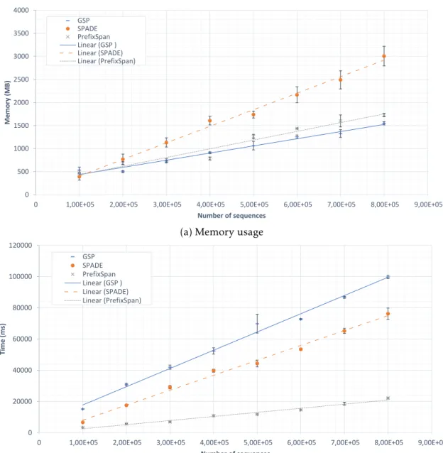
3.4.1 Long sequence

In this test, the size of the sequential database ranges from 100k sequences to 800k, being its size restricted by the available RAM. Figure 3.3represents the memory usage and computation time for the diﬀerent number of sequences. For each SPM algorithm, the

markers with the error bars represent the average values, while the lines approximate the linear trend that best fit the average values. Analysing the results depicted in Figure

3.3b, it can be seen that in terms of computational time, PrefixSpan is by far the fastest algorithm. PrefixSpan also confirms this observation as the number of sequences in the database increases from 100k to 800k. Regarding the SPADE algorithm, although slower than PrefixSpan still outperforms GSP in terms of computing time. In Figure3.3a, GSP appears to be the most eﬃcient in memory consumption, while SPADE is the one that

(52)

C H A P T E R 3 . O F F - L I N E E VA LUAT I O N O F M I N I N G A LG O R I T H M S 0 500 1000 1500 2000 2500 3000 3500 4000

0 1,00E+05 2,00E+05 3,00E+05 4,00E+05 5,00E+05 6,00E+05 7,00E+05 8,00E+05 9,00E+05

M e m or y ( M B)

Number of sequences

GSP SPADE PrefixSpan Linear (GSP ) Linear (SPADE) Linear (PrefixSpan)

(a) Memory usage

0 20000 40000 60000 80000 100000 120000

0 1,00E+05 2,00E+05 3,00E+05 4,00E+05 5,00E+05 6,00E+05 7,00E+05 8,00E+05 9,00E+05

T

ime

(m