3 On the Effectiveness of Particle Swarm Optimization and Variable Neighborhood Descent for the Continuous Flow-Shop Scheduling Problem

On the Effectiveness of Particle Swarm

Optimization and Variable Neighborhood

Descent for the Continuous Flow-Shop

Scheduling Problem

Jens Czogalla and Andreas Fink

Helmut-Schmidt-University / UniBw Hamburg Holstenhofweg 85, 22043 Hamburg, Germany [czogalla,andreas.fink]@hsu-hamburg.de

Summary. Recently population-based meta-heuristics under the cover of swarm in-telligence have gained prominence. This includes particle swarm optimization (PSO), where the search strategy draws ideas from the social behavior of organisms. While PSO has been reported as an effective search method in several papers, we are in-terested in the critical success factors of PSO for solving combinatorial optimization problems. In particular, we examine the application of PSO with different crossover operators and hybridization with variable neighborhood descent as an embedded local search procedure. Computational results are reported for the continuous (no-wait) flow-shop scheduling problem. The findings demonstrate the importance of local search as an element of the applied PSO procedures. We report new best solutions for a number of problem instances from the literature.

Key words: Flow-Shop Scheduling, Particle Swarm Optimization, Genetic Operators, Variable Neighborhood Descent, Hybridization.

3.1 Introduction

Swarm intelligence involves the design of heuristic methods for solving prob-lems in a way that is inspired by the social behavior of organisms within swarm populations, where organisms interact locally with one another and with the environment. While there is no centralized control structure, interactions be-tween the organisms may lead to the emergence of global behavior such as termite colonies building mounds, bird flocking, and fish schooling [7, 37].

Recently population-based meta-heuristics under the cover of swarm in-telligence have gained prominence. This includes particle swarm optimization (PSO), which was first introduced by Kennedy and Eberhart [14, 29] for the optimization of continuous nonlinear functions. While PSO has been reported

J. Czogalla and A. Fink: On the Effectiveness of Particle Swarm Optimization and Vari-able Neighborhood Descent for the Continuous Flow-Shop Scheduling Problem, Studies in Computational Intelligence (SCI)128, 61–89 (2008)

as an effective search method in several papers, we are interested in the critical success factors when applied to combinatorial optimization problems.

We consider the continuous (no-wait) flow-shop scheduling problem (CFSP) and analyze PSO hybridized with construction heuristics and variable neigh-borhood descent as an embedded local search procedure according to [42, 43]. Different crossover operators will be investigated and a combined crossover strategy will be derived. The analysis is based on extensive computational experiments for benchmark problem instances for the CFSP. We are able to significantly improve present best results from the literature. The findings show that local search may constitute the most important element of effective PSO approaches for combinatorial optimization problems.

In Section 3.2 we introduce the continuous flow-shop scheduling problem. In Section 3.3 we discuss PSO and extensions for combinatorial optimiza-tion problems; this includes the investigaoptimiza-tion of different crossover operators. Sections 3.4 and 3.5 are dealing with construction heuristics used to create the initial swarm population and with a local search heuristic, respectively. Computational results will be the topic of Section 3.6.

3.2 The Continuous Flow-Shop Scheduling Problem

In this section we review the continuous flow-shop scheduling problem (CFSP). First, we make a short excursion into the steel producing industry to show the motivation for the ongoing research on the continuous flow-shop scheduling problem; additionally we list applications in other branches.

3.2.1 How Iron Ore Becomes a Steel Plate

For the production of steel in a first step iron ore and coke are molted together (ironmaking). In a second step impurities (e.g., excess carbon) are removed and alloying materials (e.g., manganese, nickel) are added (steelmaking). In the further process, on the way to finished products such as steel plates and coils, the molted steel undergoes a series of operations [22] which are capital and energy extensive. Thus companies have been putting consistent emphasis on technology advances in the production process to increase productivity and to save energy [59].

integrated process of steelmaking directly connects the steelmaking furnace, the continuous caster and the hot rolling mill with hot metal flow and makes a synchronized production [59]. Such a process has many advantages over the traditional cold charge process but brings new challenges for production planning and scheduling [59].

The short excursion demonstrates necessities for the application of the no-wait restriction to real-world problems [13]. First, the production technol-ogy may require the continuous processing of jobs. Second, a lack of storage capacity may force the production schedule to adapt the no-wait restriction. However, lack of intermediate storage capacity between consecutive machines does not necessarily impose the now-wait restriction, since jobs can wait on machines (while blocking these machines) until the next machine becomes available. Hall and Sriskandarajah [22] give a survey on machine scheduling problems with blocking and no-wait characteristics. Further applications that demand a no-wait scheduling are concrete ware production [20], food process-ing [22], pharmaceutical processprocess-ing [48], chemical production [49], or more general just in time production and assembly lines.

3.2.2 Formal Description

A flow-shop scheduling problem consists of a set ofn jobs which have to be processed in an identical order on m machines. Each machine can process exactly one job at a time. The processing time of jobion machinej is given as tij with 1≤i≤nand 1≤j≤m. If a job does not need to be processed on a machine the corresponding processing time equals zero.

The continuous flow-shop scheduling problem includes no-wait restrictions for the processing of each job, i.e., once the processing of a job begins, there must not be any waiting times between the processing of any consecutive tasks of this job. Continuous processing leads to a delay dik,1 ≤ i ≤ n,1 ≤k ≤ n, i!=kon the first machine between the start of jobsi andk wheniand k are processed directly after each other. The delay can be computed as

dik= max 1≤j≤m

 j

h=1 tih−

j

h=2 tk,h−1

!

. (3.1)

The processing order of the jobs is represented as a permutation Π =< π1, ..., πn>whereπiis the job processed at thei-th position of a sched-ule. Note that the continuous flow-shop scheduling problem with makespan objective can be modeled as an asymmetric traveling salesman problem and thus can be solved by applying corresponding methods. In this chapter we consider the objective to minimize the total processing time (flow-time)

F(Π) = n

i=2

(n+ 1−i)dπ(i−1),π(i)+ n

i=1 m

j=1

The first part of Equation 3.2 sums the implied delays. Since the delay between two jobs affects all succeeding jobs the respective delay is multiplied with the number of following jobs. The second part of the formula is the constant total sum of processing times.

3.2.3 Literature Review

Since Johnson’s seminal paper [28] on the two-machine flow-shop scheduling problem the literature on flow-shop scheduling has grown rapidly. It was re-viewed by Day and Hottenstein in 1970 [12] and by Dudek et al. in 1992 [13]. Day and Hottenstein provide a classification of sequencing problems includ-ing flow-shop problems. Dudek et al. give a detailed overview on flow-shop sequencing research addressing several problem solving strategies and diverse optimization criterions. A statistical review of flow-shop literature is presented by Reisman et al. [52]. Ruiz and Maroto [53] provide a comprehensive review and evaluation of permutation flow-shop heuristics.

The continuous flow-shop scheduling problem with the objective to min-imize total flow-time as posed by van Deman and Baker [63] is theoreti-cally discussed by Gupta [21], Papadimitriou and Kanellakis [44], Szwarc [56], Adiri and Pohoryles [1], and van der Veen and van Dal [64]. Rajendran and Chauduri [50] provide a construction heuristic with two priority rules for the CFSP including computational experiments. Chen et al. [8] provide a genetic algorithm including computational results. Bertolissi [6] presents a construc-tion heuristic evaluated by computaconstruc-tional experiments. Fink and Voß [15] used several construction heuristics, tabu search, and simulated annealing and pro-vided detailed computational results. Pan et al. [42] present extensive com-putational experiments of a discrete particle swarm optimization algorithm hybridized with a construction heuristic and variable neighborhood descent.

3.3 Particle Swarm Optimization

In this section we will describe PSO in its canonical form and extensions for combinatorial optimization problems. Merkle and Middendorf [37] provide an introduction to PSO and the related literature. Kennedy and Eberhart [31] present a more detailed introduction to PSO within the scope of swarm intelligence.

3.3.1 Standard Particle Swarm Optimization

The basic idea of PSO is that a particle i_{represents a search space location}

(solution)x_i∈_Rn. Depending on its velocityv_i∈_Rn particles “fly” through

been found by the particle itself or other particles in the swarm. That is, there are two kinds of memory, individual and social, which direct the “reasoning” of the particle about the exploration of the search space.

The velocity of a particle i is canonically updated as follows:

vi:=w∗vi+c1∗U(0,1)∗(pi−xi) +c2∗U(0,1)∗(g−xi) (3.3)

wherepi is the best previous position of the particle and g is the best found

position within the swarm so far. The parameterwis called theinertia weight and represents the influence of the previous velocity. The parametersc₁ and c₂ are acceleration coefficients that determine the impact of pi and g, i.e.,

the individual and social memory, respectively. Randomness is introduced by weighting the influence of the individual and social memory by random values uniformly drawn from [0,1]. After updating the velocity, the new position of the particle is calculated as:

xi:=xi+vi. (3.4)

Listing 3.1 shows the classic PSO procedure GBEST according to Eber-hart and Kennedy [14]. After initialization of the parameters the initial pop-ulation is randomly generated and evaluated using Equation 3.2. The best position of each particle and the best position of the whole swarm is updated. Then the velocity and the position of the particles are updated according to Equations 3.3 and 3.4. After evaluating all particles a new iteration is started. The loop is repeated until a termination criterion is met (e.g., concerning the elapsed time or the number of iterations).

Listing 3.1: Standard GBEST particle swarm algorithm. i n i t i a l i z e p a r a m e t e r s

f o r a l l p a r t i c l e s i do

i n i t i a l i z e p o s i t i o n xi and v e l o c i t y vi

e v a l u a t e p a r t i c l e i end f o r

do

f o r a l l p a r t i c l e s i do update p e r s o n a l b e s t pi

update g l o b a l b e s t g end f o r

f o r a l l p a r t i c l e s i do update v e l o c i t y vi

update p o s i t i o n xi

e v a l u a t e p a r t i c l e i end f o r

w h i l e s t o p c r i t e r i o n not met

are proposed in order to improve swarm behavior and the balance between convergence speed and convergence quality. Shi and Eberhart [55] investi-gate the influence of the maximum particle velocity and the inertia weight on the ability to escape from local optima. They provide detailed computational results and give suggestions for balancing those parameters. Trelea [62] ana-lyzes PSO using standard results from dynamic system theory, discusses the tradeoff between exploration and exploitation, and presents guidelines for the selection of individual and social parameters. As swarm diversity (according to some measure of the differences between individuals of a swarm) decreases with swarm evolution, this results in a more thorough search in a restricted space while running into danger of getting stuck at local optima. Clerc [9] and Peram et al. [46] propose methods to measure and control diversity in order to prevent premature convergence.

In Kennedy and Mendes [32] and Mendes et al. [36] neighborhood relations between particles are introduced. Instead of usingg, the best solution of the swarm so far, to update the velocity of particles, the best particle in some neighborhood is used. Janson and Middendorf [27] introduce a hierarchical neighborhood. Parsopoulos and Vrahatis [45] study PSO that makes use of the combination of different neighborhoods.

Current research is also concernd with the hybridization of PSO with other heuristic methods. For example, Gimmler et al. [16] analyze the influence of the type of local search hybridized with PSO for a number of standard test functions. For machine scheduling applications, Liu et al. [33, 34] incorporate different local search approaches and an adaptive meta-Lamarckian learning strategy into PSO. Tasgetiren et al. [60,61] combine PSO with variable neigh-borhood descent.

3.3.2 Discrete Particle Swarm Optimization

Standard PSO is defined for a solution spaceRn

. In order to apply the concept of PSO for combinatorial optimization problems one may define a transforma-tion fromRn

and positions is not done directly on the solution representation, thus loosing information about the search space during the transformation process.

Therefore, it may be indicated to adapt PSO for combinatorial optimiza-tion problems by means of problem-specific operators. This approach is fol-lowed, e.g., by [42] for the no-wait flow-shop scheduling problem. It is called discrete particle swarm optimization (DPSO). In contrast to the standard PSO

updating of positions is done directly on job permutations. In this modelXi

represents as position the job permutation of thei-th particle. Using a binary

operator ⊕ with the meaning that the first operand defines the probability

that the operator given as second operand is applied, the update is done by

Xi:=c2⊕F3(c1⊕F2(w⊕F1(Xi), Pi), G). (3.5)

The first term of Equation 3.5 is λi = w⊕F1(Xi) which represents the

“velocity” of the particle. F1 is a swap operator which swaps two randomly

chosen jobs within the permutationXi of the i-th particle. The second part

δi=c1⊕F2(λi, Pi) represents the individual memory of the particle andF2is

a crossover operator applying a one-cut crossover onλi and the best position

of the particle so far. The social part is represented byXi =c2⊕F3(δi, G) with

F3as a crossover operator using a two-cut crossover onδiand the best position

of the swarmG. The parametersw,c1, and c2 determine the probabilities of

the application of swap and crossover operators, respectively.

Listing 3.2 shows the pseudo code for the DPSO according to an adapted GBEST model from [14]. Since we are interested in the impact of local search on the solution quality there is an optional local search method included. Such a local search method may be employed to improve individual solutions (e.g.,

the best swarm solution G), which results in a hybridization of the concepts

of swarm intelligence and local search.

Listing 3.2: Discrete particle swarm algorithm. i n i t i a l i z e p a r a m e t e r s

f o r a l l p a r t i c l e s i do

i n i t i a l i z e p o s i t i o n Xi; e v a l u a t e p a r t i c l e i

end f o r do

f o r a l l p a r t i c l e s i do

update p e r s o n a l b e s t Pi

update g l o b a l b e s t G

end f o r

f o r a l l p a r t i c l e s i do

update p o s i t i o n Xi

e v a l u a t e p a r t i c l e i

end f o r

l o c a l s e a r c h ( o p t i o n a l ) w h i l e s t o p c r i t e r i o n not met

procedures for different (scheduling) applications. Allahverdi and Al-Anzi [2] present a DPSO approach where particles are associated with job sequences and two velocities that correspond to probabilities of changing job positions. Results for the minimization of the maximum lateness for assembly flow-shop scheduling outperformed results obtained by tabu search and the earliest due date heuristic. Anghinolfi and Paolucci [3] investigate a DPSO approach for the single-machine total weighted tardiness scheduling problem with sequence-dependent setup times. Based on a discrete model for particle positions the velocity of a particle is interpreted as the difference in job positions of two particles. Pan et al. [43] apply DPSO to the single machine total earliness and tardiness problem with a common due date. A PSO approach for combi-natorial optimization problems employing problem independent operators is introduced in Moraglio et al. [38].

The discrete particle swarm optimization concept, with the introduction of crossover and mutation operators, is similar to other methods that fol-low the paradigm of evolutionary computation [4]. Both genetic/evolutionary algorithms and PSO are based on populations formed of individuals repre-senting solutions. The individuals are subject to some probabilistic operators such as recombination, mutation, and selection in order to evolve the pop-ulation towards better fitness values. Scatter search [17] provides a comple-mentary perspective on PSO. Scatter search generally operates on a relatively small number of solutions, called reference set. Some combination of two or more candidates from the reference set creates new solutions, which may be improved by means of local search, which is also a feature of memetic algo-rithms [25, 40]. Some of the obtained solutions may be inserted into the pop-ulation according to some rule with the aim to guarantee both high solution quality and high diversity. A further generalization is possible when following the characterization of adaptive memory programming by Taillard [58]:

1. A set of solutions or a special data structure that aggregates the particu-larities of the solutions produced by the search is memorized;

2. A provisional solution is constructed using the data in memory;

3. The provisional solution is improved using a local search algorithm or a more sophisticated meta-heuristic;

4. The new solution is included in the memory or is used to update the data structure that memorizes the search history.

3.3.3 Crossover Operators

In Equation 3.5 crossover operators are employed to create new particle po-sitions represented by permutations. There are three major interpretations for permutations [4, 39]. Depending on the problem the relevant information contained in the permutation is the adjacency relation among the elements, the relative order of the elements, or the absolute positions of the elements in the permutation. Considering Equation 3.2 the adjacency relation between the jobs has the main impact on the objective function. In addition, the ab-solute positions of jobs or sequences of jobs are of importance since delays scheduled early are weighted with a larger factor then delays scheduled late. Besides those considerations the offspring created has to be a valid permu-tation or a repair mechanism must be applied. In the following we review some recombination methods developed for permutation problems where the adjacency relation among the jobs is mainly maintained.

Theorder-based crossover(OB, see MODIFIED-CROSSOVER in [11]) takes a part of a parent, broken at random, and orders the remaining jobs in accordance with their order in the second parent [11]. To use the order-based crossover as a two-cut crossover two crossover points are chosen randomly. The jobs between the crossover points are copied to the children. Starting from the second crossover site the jobs from the second parent are copied to the child if they are not already present in the child [54]. A different crossover operator is obtained when starting at the first position (OB’).

As an example consider the two following parents and crossover sites:

Parent 1 = 0 1 2 _| 3 4 5 _| 6 7

Parent 2 = 3 7 4 _| 6 0 1 _| 2 5_.

In the first step we keep jobs 3, 4, and 5 from parent 1 and jobs 6, 0, and 1 from parent 2:

Child 1 = x x x _| 3 4 5 _| x x

Child 2 = x x x _| 6 0 1 _| x x_.

The empty spots are filled with the not yet used jobs, in the order they appear in the other parent, starting after the second crossover site:

Child 1 = 0 1 2 _| 3 4 5 _| 7 6

Child 2 = 4 5 7 _| 6 0 1 _| 2 3_.

We get different offspring when starting at the first position:

Child 1 = 7 6 0 _| 3 4 5 _| 1 2

Child 2 = 2 3 4 _| 6 0 1 _| 5 7_.

Parent 1 = 0 1 2 _| 3 4 5 _| 6 7 Parent 2 = 3 7 4 _| 6 0 1 _| 2 5_.

The first matching jobs are 3 in parent 1 and 6 in parent 2. Therefore jobs 3 and 6 are swapped. Similarly jobs 4 and 0, and 5 and 1 are exchanged:

Child 1 = 4 5 2 _| 6 0 1 _| 3 7

Child 2 = 6 7 0 _| 3 4 5 _| 2 1_.

After the exchanges each child contains ordering information partially deter-mined by each of its parents [18]. To obtain a one-cut crossover one of the crossing sites has to be the left or the right border.

ThePTL crossover_{as proposed in [43] always produces a pair of different}

permutations even from identical parents. Two crossing sites are randomly chosen. The jobs between the crossing points of the first parent are either moved to the left or the right side of the children. The remaining spots are filled with the jobs not yet present, in the order they appear in the second parent.

Parent 1 = 0 1 2 _| 3 4 5 _| 6 7

Parent 2 = 3 7 4 _| 6 0 1 _| 2 5_.

In our example we move the job sequence 345 to the left side to obtain child 1 and to the right side in order to get child 2:

Child 1 = 3 4 5 _| x x x _| x x

Child 2 = x x x _| x x 3 _| 4 5_.

The missing jobs are filled according to their appearance in the second parent:

Child 1 = 3 4 5 _| 7 6 0 _| 1 2

Child 2 = 7 6 0 _| 1 2 3 _| 4 5_.

3.4 Initial Swarm Population

The initial swarm population of a PSO implementation can be created ran-domly. More common is the employment of dedicated construction heuristics, which are often based on priority rules. With respect to the permution so-lution space, objects (jobs) are iteratively added to an incomplete schedule according to some preference relation.

The nearest neighbor heuristic (NNH), a well known construction heuris-tic related to the traveling salesman problem, can be modified to serve as construction heuristic for the CFSP. Starting with a randomly chosen job the partial scheduleΠ =!π1, ..., πk"is iteratively extended by adding an

unsched-uled jobπk+1 with a minimal delay betweenπk andπk+1. This intuitive and

Another variant of construction heuristics are simple insertion heuristics. In a first step the jobs are presorted in some way. Then the first two pre-sorted jobs are selected and the best partial sequence for these two jobs is found considering the two possible partial schedules. The relative positions of these two jobs are fixed for the remaining steps of the algorithm. At each of the following iterations of the algorithm the next unscheduled job from the presorted sequence is selected and all possible insertion positions and the resulting partial schedules are examined.

In order to create the presorted sequence of jobs the NNH can be employed (NNNEH) as shown in [42]. Another approach is described in [41], where jobs with a larger total processing time get a higher priority then jobs with less total processing time (NEH). Therefore the jobs are ordered in descending

sums of their processing timesTi=

m j₌₁ti,j.

The effectiveness of the described construction heuristics generally depends on the initial job. So we repeat the construction heuristics with each job as the first job. The resulting solutions build up the initial swarm population (i.e., we fix the size of the swarm population as the number of jobs).

3.5 Local Search

Local search algorithms are widely used to tackle hard combinatorial opti-mization problems such as the CFSP. A straightforward local search algo-rithm starts at some point in the solution space and iteratively moves to a neighboring location depending on an underlying neighborhood structure and a move selection rule. In greedy local search the current solution is replaced if a better solution with respect to the objective function is found. The search is continued until no better solution can be found in the neighborhood of the current solution. In this section we examine neighborhood structures for the CFSP and review the variable neighborhood descent approach.

A neighborhood structure is defined by using an operator that transforms

a given permutation Π into a new permutation Π∗ _{[51]. We consider two}

alternative neighborhoods, both leading to a connected search space. The

swap (or interchange) operator exchanges a pair of jobs πp1 and πp2 with

p₁ = p₂, while all the other jobs in the permutation Π remain unchanged.

The size of the swap neighborhood structure is n∗(n−1)/2. The shift (or

insertion) operator removes the jobπp1 and inserts it behind the jobπp2with

p₁ =p₂and p₁ =p₂+ 1. The size of the shift neighborhood structure results

as (n−1)2_.

Local search will be applied to the best position of the swarm G after

72 Czogalla and Fink

is not necessarily a local minimum for another neighborhood structure [23]. Consequently, VND changes the neighborhood during the search [24]. Listing 3.3 shows the pseudo code for VND. LetNk, k = 1, ..., kmax, be a set

of neighborhood structures usually ordered by the computational complexity of their application [23]. In our case N1 represents the swap neighborhood

and N₂ the shift neighborhood. The VND algorithm performs local search until a local minimum with respect to the N₁ neighborhood is found. The search process is continued within the neighborhoodN₂. If a better solution is found the search returns to the first neighborhood, otherwise the search is terminated.

The role of perturbation is to escape from local minima. Therefore the modifications produced by aperturbation should not be undone immediately by the following local search [26]. We follow the approach of [42] and use 3 to 5 random swap and 3 to 5 random shift moves as perturbation.

Listing 3.3: Variable neighborhood descent. S := p e r t u r b a t i o n (G)

e v a l u a t e S

k := 1

do

f i n d b e s t n e i g h b o r S∗ _{i n n ei g h b o r h o o d Nk o f S}

e v a l u a t e S∗

i f s o l u t i o n S∗ _{i s b e t t e r than s o l u t i o n S}

S := S∗

k := 1

e l s e

i n c r e a s e k by 1 end i f

w h i l e k≤kmax

i f s o l u t i o n S i s b e t t e r than s o l u t i o n G

G := S

end i f

3.6 Computational Results

Since we are interested in analyzing the factors contributing to the results reported in [42] we implemented DPSO for the CFSP in C#, pursuing an object-oriented approach, thus allowing easy combination of different heuris-tics. The DPSO was run on an IntelCoreT M

2 Duo processor with 3.0 GHz and 2 GB RAM under Microsoft Windows XP1_{. We applied it to}

Tail-lard’s benchmark instances2_{[57] treated as CFSP instances (as in [15]).}

1 _{In [42] DPSO was coded in Visual C++ and run on an Intel}

PentiumIV 2.4 GHz with 256 MB RAM.

In our computational experiments each configuration is evaluated by 10 runs for each problem instance. The quality of the obtained results is reported as the percentage relative deviation

∆avg= solution−solutionref

solutionref ∗100 (3.6)

wheresolutionis the total processing time generated by the variants of DPSO andsolutionref is the best result reported in [15] (using simulated annealing, tabu search, or the pilot method). The relative deviation based on the results of [15] is also the measure used in [42]. The best objective function values reported in [15] and [42] are given in Table 3.8 (Appendix of this chapter) together with the results obtained in our own new computational experiments (denoted by CF). Note that we have been able to obtain new best results for all the larger problem instances (withn= 100 andn= 200) while we have at least re-obtained present best results for the smaller problem instances.

In [15] the 3-index formulation of Picard and Queyranne [47] was used to compute optimal solutions for the 20 jobs instances (ta001–ta030) and to obtain lower bounds provided by linear programming relaxation for the 50 jobs and 100 jobs instances (ta031–ta060 and ta061–ta090, respectively). For the smaller instances with 20 jobs the best results shown in Table 3.8 correspond to optimal solutions. The lower bounds for the instances ta031–ta060 and ta061–ta090 are given in Table 3.9 (Appendix of this chapter).

The parameter values of DPSO as described in Section 3.3.2 are taken from [42] in order to enable a comparison of results. The one-cut and the two-cut crossover probabilities are set toc1=c2= 0.8. The swap probability (w)

was set towstart= 0.95 and multiplied after each iteration with a decrement factor β = 0.975 but never decreased below wmin = 0.40. As mentioned in Section 3.4 the swarm size was fixed at the number of jobs.

Since in [42] there is no detailed information about the employed crossover operators we were at first interested in evaluating different crossover operators as described in Section 3.3.3. These experiments have been performed with a random construction of the initial swarm population and without using local search. The quality of the results obtained for different iteration numbers is shown in Table 3.1 (with the computation times given in CPU seconds). No particular crossover operator is generally superior. However, it seems that the PTL crossover operator is best suited for small problem instances while OB’ and PMX work better on large instances.

Table 3.1: Comparison of different crossover operators for DPSO.

jobs PMX OB OB’ PTL

iterations ∆avg t ∆avg t ∆avg t ∆avg t

20 1000 4.99 0.01 4.88 0.04 3.48 0.03 3.84 0.03

2000 4.73 0.03 3.50 0.07 3.13 0.07 2.40 0.07

10000 4.19 0.14 1.63 0.36 2.04 0.34 1.15 0.33

50000 3.39 0.68 0.94 1.78 1.80 1.73 0.54 1.57

50 1000 9.26 0.05 17.15 0.14 8.74 0.14 15.52 0.13

2000 8.29 0.10 13.70 0.28 6.71 0.27 12.34 0.26

10000 7.72 0.49 7.52 1.46 4.71 1.31 6.60 1.24

50000 7.16 2.47 4.35 7.15 4.05 6.93 3.94 6.19

100 1000 11.56 0.16 27.43 0.48 12.51 0.46 25.51 0.42

2000 9.54 0.31 23.33 0.91 9.40 0,90 21.45 0.81

10000 8.72 1.50 13.80 4.78 5.79 4.30 13.08 3.98

50000 8.20 7.27 7.32 21.70 4.62 21.70 7.33 19.70

200 1000 14.43 0.61 38.03 1.94 17.88 1.92 36.43 1.66

2000 11.51 1.19 34.20 3.82 13.43 3.88 32.51 3.28

10000 9.08 5.88 22.79 20.44 7.09 18.14 22.40 15.91

50000 8.63 26.52 11.86 97.98 4.71 95.25 12.86 76.13

Table 3.2: Comparison of the combination of crossover operators for DPSO.

jobs PMX/OB’ PMX/PTL OB’/PMX OB’/PTL PTL/PMX PTL/OB’

iter. ∆avg t ∆avg t ∆avg t ∆avg t ∆avg t ∆avg t

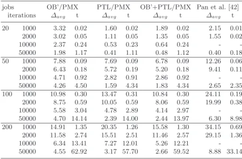
Consequently, we used PMX as two-cut crossover and randomly selected from PTL and OB’ as one-cut crossover for each particle. Table 3.3 shows the obtained results in comparison to the results reported by Pan et al. in [42] (notice that [42] do not give results for 10000 iterations). While Pan et al. re-port faster computation times, we implemented the methods using an object-oriented approach with the focus on an easy combination of the different algorithm elements without putting much value in the optimization of the code in terms of computation times. However, we mainly obtain significantly better results even when comparing on the basis of computation times.

The OB’+PTL/PMX crossover operator combination will be used through-out the remainder of this chapter and will be referred to as DPSO.

Table 3.3: Comparison of advanced crossover strategies for DPSO.

jobs OB’/PMX PTL/PMX OB’+PTL/PMX Pan et al. [42]

iterations ∆avg t ∆avg t ∆avg t ∆avg t

20 1000 3.32 0.02 1.60 0.02 1.89 0.02 2.15 0.01

2000 3.02 0.05 1.11 0.05 1.35 0.05 1.55 0.02

10000 2.37 0.24 0.53 0.23 0.64 0.24 -

-50000 1.98 1.17 0.41 1.11 0.48 1.12 0.40 0.18 50 1000 7.88 0.09 7.69 0.09 6.78 0.09 12.26 0.06 2000 6.43 0.18 5.72 0.19 5.20 0.18 9.41 0.11

10000 4.71 0.92 2.82 0.91 2.86 0.92 -

-50000 4.26 4.50 1.59 4.34 1.83 4.34 2.65 2.35 100 1000 10.98 0.30 13.47 0.31 10.84 0.30 24.11 0.19 2000 8.75 0.59 10.05 0.59 8.06 0.59 19.99 0.38

10000 5.58 3.04 4.78 2.89 4.14 2.97 -

-50000 4.70 14.14 2.39 14.00 2.44 13.97 6.30 8.98 200 1000 14.91 1.35 20.35 1.26 15.58 1.30 34.15 0.69 2000 11.58 2.74 15.51 2.51 11.46 2.57 29.15 1.36

10000 6.34 13.41 7.27 12.01 5.26 12.21 -

-50000 4.55 62.92 3.17 57.70 2.66 59.52 8.88 33.14

In accordance with [42] we also employ a dedicated construction heuris-tic to create the initial swarm population. The results presented in Table 3.4 are produced by evaluating the initial population without any iteration of DPSO performed. The insertion heuristics clearly outperform NN. Interest-ingly NEH, originally developed for the flow-shop scheduling problem with makespan criterion, performed slightly better than NNNEH. The results in-dicate that it may be advantageous to employ NEH in the initial phase of DPSO.

Table 3.4: Comparison of different construction heuristics.

jobs random NNH NEH NNNEH

∆avg t ∆avg t ∆avg t ∆avg t

20 28.54 0.00 19.04 0.00 1.71 0.00 2.10 0.00 50 47.37 0.00 25.77 0.00 4.04 0.01 4.92 0.01 100 57.29 0.00 25.65 0.01 4.62 0.04 5.58 0.04 200 65.28 0.01 19.62 0.05 3.56 0.34 4.15 0.35

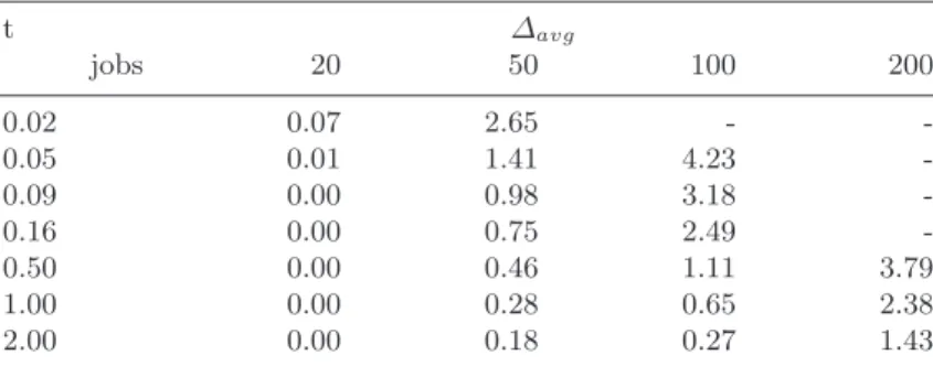
search component within DPSO (DPSOV N D) for a randomly created initial

swarm population.

Table 3.5: Results for DPSOV N D.

t ∆avg

jobs 20 50 100 200

0.02 0.07 2.65 -

-0.05 0.01 1.41 4.23

-0.09 0.00 0.98 3.18

-0.16 0.00 0.75 2.49

-0.50 0.00 0.46 1.11 3.79

1.00 0.00 0.28 0.65 2.38

2.00 0.00 0.18 0.27 1.43

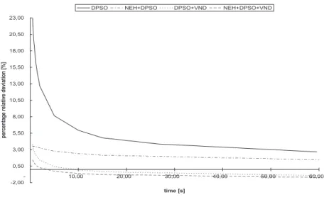
In Table 3.6 DPSO is compared to different hybridized variants. The sub-script VND denotes a possible local search component, which is applied after each iteration to the best solution of the swarm G_{; the superscript NEH}

de-notes the application of a dedicated construction heuristic. The results show that DPSO is clearly outperformed by DPSON EH

V N D. This demonstrates the

piv-otal effect of local search for the effectiveness of the applied PSO procedures. Comparing the results for the 50 jobs instances DPSO obtained∆_avg=1.83

af-ter 4.3 seconds while DPSON EH

V N Dneeded just 0.016 seconds to obtain the same

solution quality. For the 100 and 200 jobs instances DPSO was not able to obtain results with a quality comparable to solutions obtained by DPSON EH

V N D.

The effect of an increasing computational time on the solution quality, ac-cording to Table 3.6, is visualized in Figs. 3.1 – 3.4 (Appendix of this chapter). These figures show that hybridization of DPSO improves the search regardless of elapsed computation time.

Table 3.6: Comparison of DPSO with its hybridized variants.

jobs t DPSO DPSON EH _{DPSOV N D DPSO}N EH V N D

∆avg ∆avg ∆avg ∆avg

20 0.016 2.38 0.81 0.07 0.04

0.031 1.68 0.66 0.02 0.02

0.047 1.35 0.60 0.01 0.01

0.094 1.07 0.53 0.01 0.00

0.156 0.94 0.48 0.00

0.250 0.66 0.40 0.500 0.57 0.32 1.118 0.48 0.26

50 0.016 15.42 3.82 2.65 1.83

0.031 10.99 3.51 1.83 1.29

0.047 9.30 3.30 1.41 1.03

0.094 6.81 2.94 0.98 0.70

0.156 5.54 2.67 0.75 0.58

0.250 4.46 2.43 0.61 0.43

0.500 3.62 2.17 0.46 0.32

1.000 2.82 1.86 0.28 0.17

2.000 2.14 1.59 0.18 0.09

100 0.047 23.72 4.62 -

-0.094 18.30 4.51 3.18 1.92

0.156 14.57 4.34 2.49 1.39

0.250 11.73 4.11 1.89 1.07

0.500 8.72 3.64 1.11 0.59

1.000 6.25 3.13 0.65 0.27

2.000 4.76 2.70 0.27 -0.01

4.000 3.78 2.38 -0.02 -0.20

10.000 2.81 1.93 -0.25 -0.42

200 0.500 23.12 3.55 3.79

-0.750 19.62 3.51 2.88 1.04

1.000 17.57 3.48 2.38 0.78

2.000 12.64 3.26 1.43 0.28

5.000 8.15 2.77 0.41 -0.29

is performed. Therefore, instead of evolving the swarm towards better solu-tions, just the best found solution after the initialization phase is subject to a repeated application of VND. The results are presented in Table 3.7 and Figs. 3.5 – 3.8 (Appendix of this chapter). The results indicate that the ob-tained high quality solutions are mainly caused by VND (and an effective construction of the initial population by NEH).

Table 3.7: Comparison of hybridized DPSO with VND.

jobs t DPSOV N D V N D DPSON EHV N D N EHV N D

∆avg ∆avg ∆avg ∆avg

20 0.016 0.07 0.00 0.04 0.03

0.031 0.02 0.00 0.02 0.01

0.047 0.01 0.01 0.01

0.094 0.01 0.00 0.00

0.156 0.00

50 0.016 2.65 2.66 1.83 1.82

0.031 1.83 1.87 1.29 1.28

0.047 1.41 1.39 1.03 0.99

0.094 0.98 0.98 0.70 0.70

0.156 0.75 0.75 0.58 0.54

0.250 0.61 0.60 0.43 0.42

0.500 0.46 0.41 0.32 0.30

1.000 0.28 0.28 0.17 0.18

2.000 0.18 0.19 0.09 0.12

100 0.094 3.18 3.18 1.92 1.90

0.156 2.49 2.50 1.39 1.38

0.250 1.89 1.89 1.07 1.07

0.500 1.11 1.12 0.59 0.58

1.000 0.65 0.65 0.27 0.23

2.000 0.27 0.27 -0.01 -0.05

4.000 -0.02 0.00 -0.20 -0.25

10.000 -0.25 -0.26 -0.42 -0.44

200 0.500 3.79 3.80 -

-0.750 2.88 2.88 1.04 1.04

1.000 2.38 2.39 0.78 0.77

2.000 1.43 1.44 0.28 0.26

5.000 0.41 0.40 -0.29 -0.31

10.000 -0.08 -0.09 -0.62 -0.63

15.000 -0.35 -0.32 -0.77 -0.79

60.000 -0.94 -0.94 -1.22 -1.23

During our experiments we were able to improve the solutions for 74 out of 80 unsolved instances using DPSON EH

V N D. The obtained best results are listed in

Table 3.8 (Appendix of this chapter). The best solutions are printed in bold letters (with preference to the prior source in case a best solution was found repeatedly).

3.7 Conclusions

We examined the application of DPSO in combination with different crossover strategies, construction heuristics, and variable neighborhood descent. In our computational experiments DPSO without local search achieved clearly worse results than classical meta-heuristics such as, e.g., tabu search and simulated annealing [15]. Based on the computational results we conclude that some good results recently reported in different papers for DPSO may be mainly caused by the employment of local search but not by the original concepts of PSO. While we were able to significantly improve present best results from the literature by investigating and applying hybridization of DPSO with lo-cal search components (i.e., new best solutions for 74 out of 80 unsolved instances), these results are not caused by the core concepts of PSO but by the embedded local search procedure. In particular, we have found that the embedded variable neighborhood descent procedure obtained the best results when particle interactions (i.e., the core concepts of PSO) were deactivated.

With the results at hand PSO and its modified variant DPSO may not be the number one choice for solving scheduling problems. However, the performance of DPSO may be improved by a sophisticated employment of crossover operators. Further research on crossover operators (see, e.g., geo-metric PSO [38]) and on the hybridization with local search may make DPSO more effective for solving combinatorial optimization problems.

References

1. I. Adiri and D. Pohoryles. Flowshop/no-idle or no-wait scheduling to minimize the sum of completion times. Naval Research Logistics Quarterly, 29:495–504, 1982.

2. A. Allahverdi and F. S. Al-Anzi. A PSO and a tabu search heuristics for the assembly scheduling problem of the two-stage distributed database application. Computers & Operations Research, 33:1056–1080, 2006.

3. D. Anghinolfi and M. Paolucci. A new discrete particle swarm optimization approach for the total tardiness scheduling scheduling problem with sequence-dependent setup times. Working Paper, 2007.

4. T. B¨ack, D. B. Fogel, and Z. Michalewicz. Evolutionary Computation 1: Basic Algorithms and Operators. Institute of Physics Publishing, Bristol, 2000. 5. J. C. Bean. Genetic algorithms and random keys for sequencing and

6. E. Bertolissi. Heuristic algorithm for scheduling in the no-wait flow-shop. Jour-nal of Materials Processing Technology, 107:459–465, 2000.

7. E. Bonabeau, M. Dorigo, and G. Theraulaz. Swarm Intelligence: From Natural to Artificial Systems. Oxford University Press, New York, NY, 1999.

8. C.-L. Chen, R. V. Neppalli, and N. Aljaber. Genetic algorithms applied to the continuous flow shop problem.Computers & Industrial Engineering, 30:919–929, 1996.

9. M. Clerc. The swarm and the queen: Towards a deterministic and adaptive particle swarm optimization. Proceedings of the 1999 Congress on Evolutionary Computation, volume 3, pages 1951–1957, 1999.

10. P. Cowling and W. Rezig. Integration of continuous caster and hot strip mill planning for steel production. Journal of Scheduling, 3:185–208, 2000.

11. L. Davis. Applying adaptive algorithms to epistatic domains.Proceedings of the 9th International Joint Conference on Artificial Intelligence, 1:162–164, 1985. 12. J. E. Day and M. P. Hottenstein. Review of sequencing research.Naval Research

Logistics Quarterly, 17:11–39, 1970.

13. R. A. Dudek, S. S. Panwalkar, and M. L. Smith. The lessons of flowshop schedul-ing research. Operations Research, 40:7–13, 1992.

14. R. Eberhart and J. Kennedy. A new optimizer using particle swarm theory. In Sixth International Symposium on Micro Machine and Human Science, pages 39–43, 1995.

15. A. Fink and S. Voß. Solving the continuous flow-shop scheduling problem by meta-heuristics. European Journal of Operational Research, 151:400–414, 2003. 16. J. Gimmler, T. St¨utzle, and T. E. Exner. Hybrid particle swarm optimization: An examination of the influence of iterative improvement algorithms on perfor-mance. In M. Dorigo, L. M. Gambardella, M. Birattari, A. Martinoli, R. Poli, and T. St¨utzle, editors,Ant Colony Optimization and Swarm Intelligence, 5th International Workshop ANTS 2006, volume 4150 ofLecture Notes in Computer Science, pages 436–443. Springer, Berlin, 2006.

17. F. Glover, M. Laguna, and R. Marti. Scatter search. In A. Ghosh and S. Tsutsui, editors,Advances in Evolutionary Computing: Theory and Applications, pages 519–538. Springer, Berlin, 2003.

18. D. E. Goldberg. Genetic Algorithms in Search, Optimization, and Machine Learning. Addison-Wesley, Reading, MA, 1989.

19. D. E. Goldberg and R. Lingle. Alleles, loci, and the traveling salesman prob-lem. In J. Grefenstette, editor,Proceedings of the International Conference on Genetic Algorithms and Their Applications, pages 154–159. Lawrence Erlbaum Associates, Hillsdale, NJ, 1985.

20. J. Grabowski and J. Pempera. Sequencing of jobs in some production system. European Journal of Operational Research, 125:535–550, 2000.

21. J. N. D. Gupta. Optimal flowshop with no intermediate storage space. Naval Research Logistics Quarterly, 23:235–243, 1976.

22. N. G. Hall and C. Sriskandarajah. A survey of machine scheduling problems with blocking and no-wait in process. Operations Research, 44:510–525, 1996. 23. P. Hansen and N. Mladenovi´c. Variable neighborhood search. In E. K. Burke

and G. Kendall, editors,Search Methodologies. Introductory Tutorials in Opti-mization and Decision Support Techniques, pages 211–238. Springer, New York, NY, 2005.

25. W. E. Hart, N. Krasnogor, and J. E. Smith. Memetic evolutionary algorithms. In W. E. Hart, N. Krasnogor, and J. E. Smith, editors, Recent Advances in Memetic Algorithms, volume 166 ofStudies in Fuzziness and Soft Computing, pages 3–30. Springer, Berlin, 2005.

26. H. H. Hoos and T. St¨utzle. Stochastic Local Search: Foundations and Applica-tions. Elsevier, Amsterdam, 2005.

27. S. Janson and M. Middendorf. A hierarchical particle swarm optimizer and its adaptive variant. IEEE Transactions on Systems, Man, and Cybernetics. Part B: Cybernetics, 35:1272–1282, 2005.

28. S. M. Johnson. Optimal two- and three-stage production schedules with setup times included. Naval Research Logistics Quarterly, 1:61–68, 1954.

29. J. Kennedy and R. C. Eberhart. Particle swarm optimization. InProceedings of the 1995 IEEE International Conference on Neural Networks, pages 1942–1948, 1995.

30. J. Kennedy and R. C. Eberhart. A discrete binary version of the particle swarm algorithm.Proceedings of IEEE International Conference on Systems, Man, and Cybernetics, volume 5, pages 4104–4108, 1997.

31. J. Kennedy and R. C. Eberhart. Swarm Intelligence. Morgan Kaufmann Publishers, San Francisco, 2001.

32. J. Kennedy and R. Mendes. Population structure and particle swarm perfor-mance.Proceedings of the 2002 Congress on Evolutionary Computation, volume 2, pages 1671–1676, 2002.

33. B. Liu, L. Wang, and Y.-H. Jin. An effective hybrid particle swarm optimiza-tion for no-wait flow shop scheduling. The International Journal of Advanced Manufacturing Technology, 31:1001–1011, 2007.

34. B. Liu, L. Wang, and Y.-H. Jin. An effective PSO-based memetic algorithm for flow shop scheduling.IEEE Transaction on Systems, Man, and Cybernetics. Part B: Cybernetics, 37:18–27, 2007.

35. H. R. Louren¸co, O. C. Martin, and T. St¨utzle. Iterated local search. In F. Glover and G. A. Kochenberger, editors,Handbook on Meta-heuristics, pages 321–353. Kluwer Academic Publishers, Norwell, MA, 2002.

36. R. Mendes, J. Kennedy, and J. Neves. The fully informed particle swarm: Simpler, maybe better. IEEE Transactions on Evolutionary Computation, 8: 204–210, 2004.

37. D. Merkle and M. Middendorf. Swarm intelligence. In E. K. Burke and G. Kendall, editors,Search Methodologies. Introductory Tutorials in Optimiza-tion and Decision Support Techniques, pages 401–435. Springer, New York, NY, 2005.

38. A. Moraglio, C. Di Chio, and R. Poli. Geometric particle swarm optimisation. In M. Ebner, M. O’Neill, A. Ek´art, L. Vanneschi, and A. I. Esparcia-Alc´azar, editors,Proceedings of the 10th European Conference on Genetic Programming, volume 4445 of Lecture Notes in Computer Science, pages 125–136. Springer, Berlin, 2007.

39. A. Moraglio and R. Poli. Topological crossover for the permutation represen-tation. In F. Rothlauf et al., editors, Genetic and Evolutionary Computation Conference, GECCO 2005 Workshop Proceedings, 2005, pages 332–338. ACM Press, New York, NY, 2005.

82 Czogalla and Fink

Concurrent Computation Program, California Institute of Technology, Pasadena, 1989.

41. M. Nawaz, E. E. Enscore, jr., and I. Ham. A heuristic algorithm for the m-machine, n-job flow-shop sequencing problem. Omega, 11:91–95, 1983. 42. Q.-K. Pan, M. F. Tasgetiren, and Y.-C. Liang. A discrete particle swarm

opti-mization algorithm for the no-wait flowshop scheduling problem.Working Pa-per, 2005.

43. Q.-K. Pan, M. Tasgetiren, and Y.-C. Liang. A discrete particle swarm optimiza-tion algorithm for single machine total earliness and tardiness problem with a common due date. InIEEE Congress on Evolutionary Computation 2006, pages 3281–3288, 2006.

44. C. H. Papadimitriou and P. C. Kanellakis. Flowshop scheduling with limited temporary storage. Journal of the ACM, 27:533–549, 1980.

45. K. E. Parsopoulos and M. N. Vrahatis. Studying the performance of unified par-ticle swarm optimization on the single machine total weighted tardiness problem. In A. Sattar and B.-H. Kang, editors,AI 2006: Advances in Artificial Intelli-gence, volume 4304 ofLecture Notes in Artificial Intelligence, pages 760–769. Springer, Berlin, 2006.

46. T. Peram, K. Veeramachaneni, and K. M. Chilukuri. Fitness-distance-ratio based particle swarm optimization. Proceedings of the 2003 IEEE Swarm Intel-ligence Symposium, pages 174–181, 2003.

47. J.-C. Picard and M. Queyranne. The time-dependent traveling salesman prob-lem and its application to the tardiness probprob-lem in one-machine scheduling. Operations Research, 26:86–110, 1978.

48. W. Raaymakers and J. Hoogeveen. Scheduling multipurpose batch process in-dustries with no-wait restrictions by simulated annealing. European Journal of Operational Research, 126:131–151, 2000.

49. C. Rajendran. A no-wait flowshop scheduling heuristic to minimize makespan. Journal of the Operational Research Society, 45:472–478, 1994.

50. C. Rajendran and D. Chauduri. Heuristic algorithms for continuous flow-shop problem. Naval Research Logistics Quarterly, 37:695–705, 1990.

51. C. R. Reeves. Fitness landscapes. In E. K. Burke and G. Kendall, editors, Search Methodologies: Introductory Tutorials in Optimization and Decision Sup-port Techniques, pages 587–610. Springer, Berlin, 2005.

52. A. Reisman, A. Kumar, and J. Motwani. Flowshop scheduling/sequencing re-search: A statistical review of the literature, 1952-1994. IEEE Transactions on Engineering Management, 44:316–329, 1997.

53. R. Ruiz and C. Maroto. A comprehensive review and evaluation of permutation flowshop heuristics. European Journal of Operational Research, 165:479–494, 2005.

54. K. Sastry, D. Goldberg, and G. Kendall. Genetic algorithms. In E. K. Burke and G. Kendall, editors,Search Methodologies. Introductory Tutorials in Opti-mization and Decision Support Techniques, pages 96–125. Springer, New York, NY, 2005.

56. W. Szwarc. A note on the flow-shop problem without interruptions in job processing. Naval Research Logistics Quarterly, 28:665–669, 1981.

57. E. Taillard. Benchmarks for basic scheduling problems. European Journal of Operational Research, 64:278–285, 1993.

58. E. D. Taillard, L. M. Gambardella, M. Gendreau, and J.-Y. Potvin. Adaptive memory programming: A unified view of meta-heuristics. European Journal of Operational Research, 135:1–16, 2001.

59. L. Tang, J. Liu, A. Rong, and Z. Yang. A review of planning and schedul-ing systems and methods for integrated steel production. European Journal of Operational Research, 133:1–20, 2001.

60. M. Tasgetiren, M. Sevkli, Y.-C. Liang, and G. Gencyilmaz. Particle swarm optimization algorithm for single machine total weighted tardiness problem. In Proceedings of the 2004 Congress on Evolutionary Computation, volume 2, pages 1412–1419, 2004.

61. M. F. Tasgetiren, Y.-C. Liang, M. Sevkli, and G. Gencyilmaz. A particle swarm optimization algorithm for makespan and total flowtime minimization in the permutation flowshop sequencing problem. European Journal of Operational Research, 177:1930–1947, 2007.

62. I. C. Trelea. The particle swarm optimization algorithm: convergence analysis and parameter selection. Information Processing Letters, 85:317–325, 2003. 63. J. M. van Deman and K. R. Baker. Minimizing mean flowtime in the flow shop

with no intermediate queues. AIIE Transactions, 6:28–34, 1974.

Figures and Tables

0,00 0,20 0,40 0,60 0,80 1,00 time [s] p e rc e n ta g e r e la ti v e d e v ia ti o n [ % ]

DPSO NEH+DPSO DPSO+VND NEH+DPSO+VND

Fig. 3.1: Comparison of DPSO with its hybridized variants for 20 jobs instances.

0,00 1,50 3,00 4,50 6,00 7,50 9,00 10,50 12,00 13,50 15,00

0,00 0,50 1,00 1,50 2,00 2,50 3,00 3,50 4,00 time [s] pe rc en ta ge r el at iv e de vi at io n [% ]

DPSO NEH+DPSO DPSO+VND NEH+DPSO+VND

-2,00 1,00 4,00 7 ,00 10,00 13,00 16,00 19,00 22,00

- 1,00 2,00 3,00 4,00 5,00 6,00 7,00 8,00 9,00 10,00

time [s] p er ce n ta g e re la ti ve d ev ia ti o n [ % ]

DPSO NEH+DPSO DPSO+VND NEH+DPSO+VND

Fig. 3.3: Comparison of DPSO with its hybridized variants for 100 jobs instances.

-2,00 0,50 3,00 5,50 8,00 10,50 13,00 15,50 18,00 20,50 23,00

- 10,00 20,00 30,00 40,00 50,00 60,00

time [s] p er ce n ta g e re la ti ve d ev ia ti o n [ % ]

DPSO NEH+DPSO DPSO+VND NEH+DPSO+VND

0,00 0,02 0,04 0,06 0,08 0,10 0,12 0,14 0,16 0,18 0,20

- 0,05 0,10 0,15 0,20 0,25

time [s]

pe

rc

en

ta

ge

r

el

at

iv

e

de

vi

at

io

n

[%

]

VND DPSO+VND NEH+VND NEH+DPSO+VND

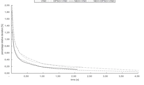
Fig. 3.5: Comparison of hybridized variants of DPSO with NEH & VND (and DPSO mechanisms turned off) for 20 jobs instances.

0,00 0,20 0,40 0,60 0,80 1,00 1,20 1,40 1,60 1,80 2,00

- 0,50 1,00 1,50 2,00 2,50 3,00 3,50 4,00 time [s]

pe

rc

en

ta

ge

r

el

at

iv

e

de

vi

at

io

n

[%

]

VND DPSO+VND NEH+VND NEH+DPSO+VND

-0,50 0,00 0,50 1,00 1,50 2,00 2,50 3,00 3,50

- 1,00 2,00 3,00 4,00 5,00 6,00 7,00 8,00 9,00 10,00

time [s]

pe

rc

en

ta

ge

r

el

at

iv

e

de

vi

at

io

n

[%

]

VND DPSO+VND NEH+VND NEH+DPSO+VND

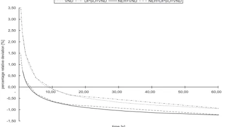
Fig. 3.7: Comparison of hybridized variants of DPSO with NEH & VND (and DPSO mechanisms turned off) for 100 jobs instances.

-1,50 -1,00 -0,50 0,00 0,50 1,00 1,50 2,00 2,50 3,00 3,50

- 10,00 20,00 30,00 40,00 50,00 60,00

time [s]

pe

rc

en

ta

ge

r

el

at

iv

e

de

vi

at

io

n

[%

]

VND DPSO+VND NEH+VND NEH+DPSO+VND

Table 3.8: Best known solutions for Taillard’s benchmark instances.

Instance CF PTL [42] FV [15] Instance CF PTL [42] FV [15]

Ta001 15674 15674 15674 Ta061 303273 304721 308052 Ta002 17250 17250 17250 Ta062 297723 297816 302386 Ta003 15821 15821 15821 Ta063 291033 292227 295239 Ta004 17970 17970 17970 Ta064 276224 276507 278811 Ta005 15317 15317 15317 Ta065 289639 289735 292757 Ta006 15501 15501 15501 _Ta066 286860 _{287133 290819} Ta007 15693 15693 15693 Ta067 297466 298039 300068 Ta008 15955 15955 15955 Ta068 286961 287073 291859 Ta009 16385 16385 16385 Ta069 303357 303550 307650 Ta010 15329 15329 15329 Ta070 297367 297486 301942 Ta011 25205 25205 25205 Ta071 408840 409116 412700 Ta012 26342 26342 26342 Ta072 389674 391125 394562 Ta013 22910 22910 22910 _Ta073 402489 _{403157 405878} Ta014 22243 22243 22243 Ta074 418588 419711 422301 Ta015 23150 23150 23150 Ta075 398088 398544 400175 Ta016 22011 22011 22011 Ta076 388344 388667 391359 Ta017 21939 21939 21939 Ta077 390162 390350 394179 Ta018 24158 24158 24158 Ta078 399060 399549 402025 Ta019 23501 23501 23501 _Ta079 413699 _{413802 416833} Ta020 24597 24597 24597 _Ta080 408855 _{409007 410372} Ta021 38597 38597 38597 Ta081 556991 559288 562150 Ta022 37571 37571 37571 Ta082 561424 563231 563923 Ta023 38312 38312 38312 Ta083 558763 558870 562404 Ta024 38802 38802 38802 Ta084 558797 560726 562918 Ta025 39012 39012 39012 Ta085 552417 552861 556311 Ta026 38562 38562 38562 _Ta086 559950 _{560296 562253} Ta027 39663 39663 39663 Ta087 569714 571150 574102 Ta028 37000 37000 37000 Ta088 573225 573834 578119 Ta029 39228 39228 39228 Ta089 559989 560095 564803 Ta030 37931 37931 37931 Ta090 568013 570292 572798 Ta031 75668 75682 76016 Ta091 1488029 1495277 1521201 Ta032 82874 82874 83403 Ta092 1474847 1479484 1516009 Ta033 78103 78103 _{78282 Ta093} 1488869 _{1495698 1515535} Ta034 82413 82533 82737 Ta094 1458413 1467327 1489457 Ta035 83476 83761 83901 Ta095 1471096 1471586 1513281 Ta036 80671 80682 80924 Ta096 1468536 1472890 1508331 Ta037 78604 78643 78791 Ta097 1502101 1512442 1541419 Ta038 78726 78821 79007 Ta098 1493418 1497303 1533397 Ta039 75647 _{75851 75842 Ta099} 1475304 _{1480535 1507422} Ta040 83430 _{83619 83829 Ta100} 1486285 _{1492115 1520800} Ta041 114051 114091 114398 Ta101 1983177 1991539 2012785 Ta042 112116 112180 112725 Ta102 2024959 2031167 2057409 Ta043 105345 105365 105433 Ta103 2018601 2019902 2050169 Ta044 113206 113427 113540 Ta104 2006227 2016685 2040946 Ta045 115295 115425 115441 Ta105 2006481 2012495 2027138 Ta046 112477 _{112871 112645 Ta106} 2014598 _{2022120 2046542} Ta047 116521 116631 116560 Ta107 2015856 2020692 2045906 Ta048 114944 114984 115056 Ta108 2020281 2026184 2044218 Ta049 110367 110367 110482 Ta109 2000386 2010833 2037040 Ta050 113427 113427 113462 Ta110 2018903 2025832 2046966 Ta051 172831 172896 172845

Table 3.9: Lower bounds for Taillard’s benchmark instances (n= 50,n= 100).

Instance LB Instance LB