On the cyclicality of social expenditure : new time-varying evidence from developing economies

(1)

REM WORKING PAPER SERIES

On the Cyclicality of Social Expenditure: New Time-Varying

evidence from Developing Economies

João Tovar Jalles

REM Working Paper 082-2019

May 2019

REM – Research in Economics and Mathematics

Rua Miguel Lúpi 20, 1249-078 Lisboa,

Portugal

ISSN 2184-108X

Any opinions expressed are those of the authors and not those of REM. Short, up to two paragraphs can be cited provided that full credit is given to the authors.

(2)

O

N THE

C

YCLICALITY OF

S

OCIAL

E

XPENDITURE

:

N

EW

T

IME

-V

ARYING

E

VIDENCE FROM

D

EVELOPING

E

CONOMIES

*

João Tovar Jalles

$

March 2019 Abstract

This paper provides a novel dataset of time-varying measures of social spending cyclicality for an unbalanced panel of 45 developing economies from 1982 to 2012. More specifically, we focus on four categories of government social expenditure: health, social protection, pensions and education. We find that social spending has generally been acyclical over time in developing countries, with the exception of spending on pensions. However, sample averages high marked heterogeneity across countries with the majority showing procyclical behaviour in different social spending categories. In addition, by means of weighted least squares panel regressions with country and time effects, we find that the degree of social spending [pro]cyclicality is generally negatively associated with financial deepening, the level of economic development, trade openness, government size as well as political constraints on the executive.

Keywords: education, health, pensions, time-varying coefficients, weighted least squares, financial development, institutions

JEL codes: C22, C23, H50, H60, H62

*_{The opinions expressed herein are those of the author and do not necessarily reflect those of the author´s employers.} All remaining errors are the author´s sole responsibility.

$_{REM – Research in Economics and Mathematics, UECE – Research Unit on Complexity and Economics. Rua Miguel} Lupi 20, 1249-078 Lisbon, Portugal. UECE is supported by FCT (Fundação para a Ciência e a Tecnologia, Portugal), Economics for Policy and Centre for Globalization and Governance, Nova School of Business and Economics, Rua da Holanda, Carcavelos, 2775-405, Portugal. email: joaojalles@gmail.com

(3)

2 1. Introduction

Understanding the cyclicality of government expenditure is relevant from a policy making perspective. Expenditure patterns may change due to policy makers’ discretionary actions or as a result of the operation of automatic stabilizers (Granado et al., 2013). Government’s social spending policy has a stabilizing effect on the economy if one of its categories (e.g. spending on social protection or health) increases when output growth increases and falls when output growth declines (Furceri, 2010). The more countercyclical government social spending is, the higher its stabilizing effect—a relatively high level of government social spending when private demand is low will stabilize aggregate demand. Most of the empirical studies looking at the cyclical properties of government expenditure (and its components) typically uncover i) an acyclical or countercyclical behaviour for advanced countries (see e.g. Hallerberg and Strauch, 2002) and ii) a procyclical pattern for developing ones (Gavin et al., 1996; Kaminsky et al., 2005; Alesina and Tabellini, 2005). A number of explanations have been put forward to justify the different cyclical patterns in different groups of countries (see section 2 for more details).

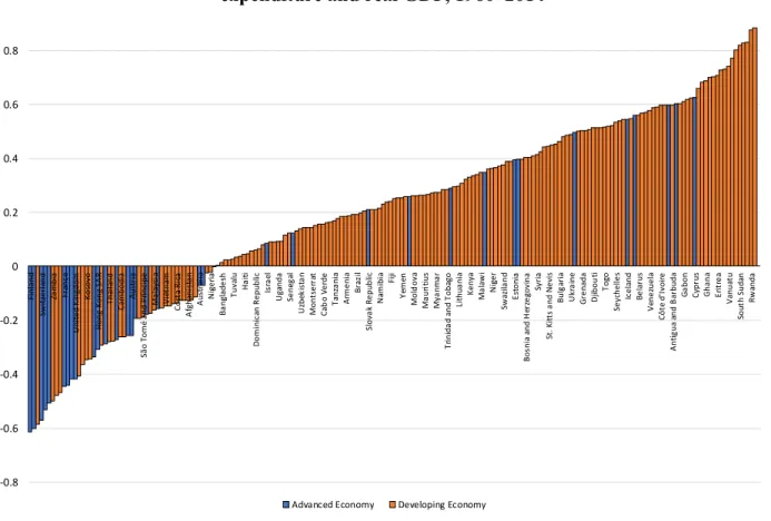
Focusing on government spending, the contrast between the two groups of countries can be clearly seen in Figure 1, which updates evidence presented in Kaminsky et al. (2004) and Frankel et al. (2013). The figure depicts the correlation between (the cyclical components of) government spending and GDP for 196 countries for the period 1960-2014. Blue bars represent advanced economies while orange bars represent developing ones. A positive (negative) correlation indicates procyclical (countercyclical) government spending. The majority of (developing) countries depicts a procyclical fiscal policy.

(4)

3

Figure 1. Country correlations between the cyclical components of real government expenditure and real GDP, 1960–2014

Notes: Dark bars are advanced economies and light ones are developing ones. The cyclical components have been estimated using the Hodrick–Prescott Filter. A positive (negative) correlation indicates procyclical (countercyclical) fiscal policy. Real government expenditure is defined as central government expenditure and net lending deflated by the GDP deflator. Data from IMF’s WEO and IFS.

Most empirical studies on this topic can be split in two: i) those that document the cyclical properties of fiscal policy and/or its components; ii) and those that inspect their determinants (typically using cross-country regressions on large datasets). The overwhelming share of papers has focused, for reasons related to data availability and quality, to analyses of European or OECD countries more generally. In this paper we ask two main questions. First, how stabilizing is de facto government’s social policy in developing countries and how has its cyclicality varied over time, between countries and around business cycles’ turning points? Second, which macroeconomic, financial, institutional and political variables determine the degree of cyclicality of government’s social spending in developing countries?

We try to answer these two questions using a novel empirical strategy and estimating time-varying measures of different categories of social spending cyclicality for an unbalanced panel of 45 emerging and low-income countries from 1982 to 2012.1_{To the best of our knowledge, this is}

1_{The selection of countries was based on the criteria of having at least 20 continuous time-series observations for a} given social spending category so as to be able to properly estimate a time-varying coefficients model.

-0.8 -0.6 -0.4 -0.2 0 0.2 0.4 0.6 0.8 Fi nl an d Sw itz er la nd Za m bi a Fr an ce U ni te d Ki ng do m Ko so vo Ho ng K on g SA R Th ai la nd Ca m bo di a Au st ri a Sã o To m é an d Pr ín ci pe M al ay si a Vi et na m Co st a Ri ca A fg ha ni st an A us tr al ia N ig er ia Ba ng la de sh Tu va lu H ai ti Do m in ic an R ep ub lic Is ra el U ga nd a Se ne ga l U zb ek is ta n M on ts er ra t Ca b o Ve rd e Ta nz an ia Ar m en ia Br az il Sl ov ak R ep ub lic N am ib ia _Fiji Ye m en M ol d ov a M au ri tiu s M ya nm ar Tr in id ad a nd T ob ag o Li th ua ni a Ke ny a M al aw i N ig er Sw az ila nd Es to ni a Bo sn ia a nd H er ze go vi na Sy ria St . K itt s an d N ev is Bu lg ar ia U kr ai ne G re na da D jib ou ti To go Se yc he lle s Ic el an d Be la ru s Ve ne zu el a Cô te d 'Iv oi re A nt ig ua a nd B ar bu da Ga bo n Cy pr us G ha na Er it re a Va nu at u So ut h Su da n Rw an da

(5)

4

the first paper that estimates time-varying measures of different categories of social spending cyclicality for a large set of developing economies. In addition, we examine which are the most relevant determinants of the varying measures of social spending cyclicality. The use of time-varying measures of social spending cyclicality overcomes the major limitation of previous studies assessing the drivers of fiscal cyclicality that rely on cross-country regressions and therefore are not able to account for country-specific as well as global factors.

The key findings of the paper are as follows. First, social spending has generally been acyclical over time in developing countries, with the exception of spending on pensions. However, sample averages high marked heterogeneity across countries with the majority showing procyclical behaviour in different social spending categories. In addition, we find that the degree of social spending [pro]cyclicality is generally negatively associated with financial deepening, the level of economic development, trade openness, government size as well as political constraints on the executive. These results depend on some structural characteristics of a given economy such as its indebtedness level, the stage of development of financial markets and the quality of its institutions.

The remainder of the paper is structured as follows. Section 2 reviews the literature. Section 3 outlines the empirical methodology and discusses the data used. Section 4 presents some key stylized facts and discusses the main empirical results. The last section concludes.

2. Literature Review

Most discussions on the cyclicality patterns of fiscal policy in general are centred around two main theories linking it to business cycle fluctuations: the Keynesian approach and the Neoclassical tax-smoothing model (Barro, 1979). The Keynesians posit that governments should spend and tax countercyclically, i.e., boosting demand through increased spending or lower taxes during a recession and doing the opposite during booms (Prasad and Gerecke, 2010). In contrast, Barro’s tax-smoothing model recommends acyclical fiscal policy that helps keep government expenditure and tax rates constant regardless of output fluctuations.

As far as expenditure policy is concerned, in order to stabilize the economy, governments should increase public spending during an economic downturn and vice versa. This would be a desirable feature from a fiscal stabilization perspective - and indeed a characteristics present is advanced economies (Talvi and Vegh, 2005; Staehr, 2008; Egert, 2012). However, Gavin, Hausmann, Perotti and Talvi (1996)2_{called the attention to the fact that the reality in many}

developing countries was of procyclicality in the conduct of expenditure policy (Kaminsky, Reinhart and Vegh, 2004; Talvi and Vegh, 2005; Ilzetzki and Vegh, 2008; Diallo, 2009; Abdih et al., 2010). In other words, we observe in developing countries spending indicators comoving positively with the business cycle, a behaviour that reinforces cycles and exacerbates booms and aggravates busts. This procyclical patterns was particularly evident in periods of financial distress

2_{These authors were the first to notice the procyclical phenomenon in Latin American countries that differed} substantially from that in the OECD countries and did not conform with either Keynesian or Barro prescriptions.

(6)

5

(Real and Vicente, 2008; Vegh and Vuletin, 2012). 3_{Recently, Frankel, Vegh and Vuletin (2013)}

showed that over the last decade about one third of the developing world could escape the procyclicality trap and engage in countercyclical fiscal policy.

Now, an important component of countercyclical fiscal policy is countercyclical social policy, which includes unemployment benefits and other social transfers, expenditure on health, education and social protection. Some studies have conducted cross-country analyses on the cyclicality of social expenditures. For instance, Braun and Gresia (2003) compared the cyclicality of social expenditures in Latin American and the Caribbean with that in the OECD countries. Molina (2003) showed that social spending was cut disproportionally following the fall in GDP during the 1980s Latin America debt crisis. Doytch et al. (2010) analysed the link between indicators of the business cycle and social spending with a focus on health and education. In middle income countries, education spending was found to be acyclical while health spending was found to be procyclical, with the pattern reversing in low income countries. Granado et al. (2013) found that spending on education and health was procyclical in developing countries.

A number of explanations have been put forward to justify different cyclical fiscal patterns in different groups of countries. Inadequate access to international credit markets and lack of financial depth (Gavin et al., 1996; Gavin and Perotti, 1997; Calderon and Schmidt-Hebbel, 2008) as well as political distortions and weak institutions (Tornell and Lane, 19994; Alesina, Tabellini

and Campante, 2008; Talvi and Vegh, 2005; Acemoglu et al. 2013; and Fatas and Mihov 2013; Abbott, Cabral, Jones, Palacios, 2015) are the two main reasons behind the observation of fiscal procyclicality in developing countries. The first argument relates to the limited access to the international market with the credit rationing imposed by investors (especially during an economic downturn) limiting the ability of the government to conduct countercyclical fiscal policy. The second reason has been built around the perception that political issues and weak institutions are prime contributors to procyclical fiscal policies (Alesina et al., 2008). It also relates to the observation that higher fiscal counter-cyclicality was found in more developed countries and these tend to be characterized by better institutions (or of higher quality). Moreover, political systems in which power is diffused among many agents will witness a higher degree of fiscal procyclicality in contrast to a unitary system.

3_{Emerging markets in particular, have a high reliance on external debt for financing government expenditures} (Reinhart and Rogoff, 2011) and face countercyclical interest rates, meaning high borrowing costs during recessions exacerbate the financing problem. See Neumeyer and Perri (2005) and Uribe and Yue (2006) for evidence of countercyclical interest rates.

4_{Tornell and Lane (1999) seminal framework highlighted different political blocs competing for a share of fiscal} revenues. They argued that competition among these fiscal blocs increased during the boom period. This approach resulted in increased government expenditure as compared to increased general income – an effect known as voracity.

(7)

6 3. Empirical Methodology and Data 3.1 Time-Varying Social Spending Cyclicality

Social spending has a stabilizing effect on the economy if one of its categories (e.g. spending on education or health - expressed in percentage of GDP)- increases when output growth declines and falls when output growth increases. The more countercyclical government social spending is, the higher its stabilizing effect—a relatively high level of government social spending when private demand is low will stabilize aggregate demand. In contrast, government social spending is destabilizing when it is procyclical. Our first step consists of assessing the degree of social spending cyclicality in each country i by estimating the response of changes in a given social spending category to changes in economic activity, as follows5_:

∆ln(𝑠 ) = 𝛼 + 𝛽 ∆ln (𝑦 ) + 𝜀 (1)

where s is a social spending category (expressed in real terms using the GDP deflator), ∆ln (𝑦 ) is a measure of changes in economic activity—proxied by real GDP growth—and 𝛽 measures the degree of social spending cyclicality in country i: 𝛽 > 0 denotes social spending procyclicality; 𝛽 < 0 denotes social spending counter-cyclicality. We look at four social spending categories, namely: health, social protection, pensions and education. Data for these variables, as well as for real GDP and its deflator are taken from the IMF WEO database.

We then generalize equation (1) by introducing the assumption that the regression coefficients may vary over time:

∆ln(𝑠 ) = 𝛼 + 𝛽 ∆ln (𝑦 ) + 𝜀 (2)

The coefficient of interest 𝛽 is assumed to change slowly and unsystematically over time and its conditional expected value today is equal to yesterday’s value. The change of the coefficient 𝛽 is denoted by 𝑣_, , which is assumed to be normally distributed with expectation zero and variance 𝜎 :

𝛽 = 𝛽 + 𝑣 (3)

Equation (2) and (3) are jointly estimated using the Varying-Coefficient model proposed by Schlicht (2003). In this approach the variances 𝜎 are calculated by a method-of-moments estimator that coincides with the maximum-likelihood estimator via the Kalman filter if the time series are sufficiently long and if the variance ratios are properly estimated (see Schlicht, 2003; Schlicht and Ludsteck, 2006 for more details).6_{In addition, the Schlicht approach is useful}

5_{Several papers have employed this first difference specification – see e.g. Lane (1998), Woo (2009) and Thornton} (2008).

6_{The approach proposed by Schlicht (2003) is very similar to that used by Aghion and Marinescu (2008). The main} difference is in the computation of the variances 𝜎 . Aghion and Marinescu (2008) uses the Markov Chain Monte

(8)

7

because: i) it does not require knowledge of initial values prior to the estimation procedure. Instead, both the variance ratios and the coefficients are estimated simultaneously; ii) the property of the estimator that the time averages of the estimated varying coefficients are equal to its time-invariant counterparts, permits easy interpretation of the results in relation to time-time-invariant results. The model described in equation (2) and (3) generalizes equation (1), which is obtained as a special case when the variance of the disturbances in the coefficients approaches to zero.

As discussed by Aghion and Marinescu (2008), this method has several advantages compared to other methods to compute time-varying coefficients such as rolling windows and Gaussian methods. First, it allows using all observations in the sample to estimate the degree of social spending cyclicality in each year—which by construction is not possible in the rolling windows approach. Second, changes in the degree of social spending cyclicality in a given year come from innovations in the same year, rather than from shocks occurring in neighbouring years. Third, it reflects the fact that changes in policy are slows and depends on the immediate past. Fourth, it reduces reverse causality problems when social spending cyclicality is used as explanatory variable as it depends on its own past (see next sub-section).

3.2 Determinants of Social Spending Cyclicality

The second step in our exercise is to empirically assess the importance of various macroeconomic, financial and institutional factors in affecting the degree of (the time-varying) social spending cyclicality. There is only one study – to the best of our knowledge – that assessed the determinants of fiscal cyclicality at the general level (i.e. not looking and public expenditure composition) using time-varying measures. This paper is by Aghion and Marinescu (2008) but they have focused on a subset of advanced economies. We estimate the following regression on an unbalanced panel comprised of 45 countries for which we have estimates of social spending cyclicality for at least 20 years7_:

𝛽 = 𝛿 + 𝛾 + 𝜽′𝑿_𝒊𝒕+ 𝜖 (4)

where 𝛽 are the time-varying coefficient estimates obtained from equation (2), 𝛿 are country-fixed effects to capture unobserved heterogeneity across countries, and time-unvarying factors such as geographical variables; 𝛾 are time-fixed effects to control for global shocks; and 𝑿_𝒊𝒕 is a vector of time-varying macroeconomic, financial and institutional variables: 8

Carlo (MCMC) method to approximate these variances, while Schlicht (2003) uses a method-of-moments estimator. Moreover, the Kalman filter as implemented in common econometric packages typically uses the diffusion of priors for its initiation, but it still produces many corner solutions and often does not achieve convergence. Schlicht and Ludsteck (2006) compare the performance of the moment estimator and the Kalman smoother in terms of the mean squared error on simulated data, and they conclude that the moment estimator outperforms the Kalman filter on small samples with a size of up to 100 observations.

7_{List of countries is provided in the Appendix.}

(9)

8

As far as macroeconomic variables are concerned, we include real GDP per capita as a proxy of economic development in line with Talvi and Vegh (2005) and Mpatswe, Tapsoba and York (2011). This variable is expected to be negatively correlated with procyclicality. Government size has typically been found to be the most important driver (Gali, 1994; Debrun et al., 2008; Debrun and Kapoor, 2011; Woo, 2009; Furceri, 2010; Afonso and Jalles, 2013; Fatas and Mihov, 2013). We include the government expenditures-to-GDP ratio which is expected to negatively affect the degree of procyclicality under the assumption of unitary elasticity of taxes to GDP. In order to reduce reverse causality, all the macroeconomic variables enter with one lag.9

Several variables have been used as proxies of the stringency of financial constraints. One is the degree of trade openness (defined as the sum of exports and imports over GDP) as a measure of access to foreign capital markets: economies that are more open to trade tend to be more exposed to external shocks and may use more actively fiscal policies in order to provide increased stabilization (Rodrik, 1998; Lane, 2003; Woo, 2009). Another is capital account openness (proxied by the Chinn-Ito index) which was found to affect fiscal cyclicality as foreign capital tends to flow in (out) during expansions (recessions), therefore increasing the cost of financing counter-cyclical fiscal policies (Aghion and Marinescu, 2008). We also use a measure of financial deepening the private credit-to-GDP ratio, as a higher level of financial development positively influences the ability of the government to borrow during downturns, and therefore it is expected to decrease fiscal procyclicality. Finally, Leaven and Valencia (2010) financial crises dummies are included but their effect on fiscal cyclicality is ambiguous a priori. On the one hand, governments would be willing to run expansionary fiscal policies to offset the contractionary effects of the crises. On the other hand, the cost of financing countercyclical fiscal policies may increase during crises, particularly in countries with high debt levels.10

Institutional variables comprise of the following. We include dummies for the occurrence of executive and legislative elections since during elections politicians may be tempted to change fiscal components for electoral reasons and not necessarily for macroeconomic stabilization purposes (Drazen 2000; Persson and Tabellini, 2000). Then, following Acemoglu et al. (2013) and Fatas and Mihov (2013) we include a proxy for constrains on the executive that captures potential veto points on the decisions of the executive. This variable is likely to reduce spending volatility and negatively influence procyclicality. Other political variables are the margin of majority, proportional representation, the existence of parliamentary regimes, checks and balances, polity2 indicator and regime durability.

The dependent variable in equation (4) is based on estimates which means that the residuals from that regression can be thought of as having two components. The first is sampling error while the second is the random shock that would have been obtained even if the dependent variable was

9_{Recall additionally, that the TVC method employed to get our dependent variable, also has the property of} minimizing reverse causality problems since the time-varying estimated cyclicality coefficient depends on its own the past (see equation 3 and explanations in section 3.1). Similar results are obtained using contemporaneous regressors (results available upon request).

10_{Other financial variables that have been employed include credit ratings and the spread of sovereign debt over the} US debt (Alesina et al., 2008). We are not using these since they would dramatically reduce the sample size.

(10)

9

observed directly as opposed to estimated. To account for the presence of this un-measurable error term, equation (4) is estimated using Weighted Least Squares (WLS). Specifically, the WLS estimator assumes that the errors 𝜖 in equation (1) are distributed as 𝜖 ~𝑁(0, 𝜎 𝑠⁄ ), where 𝑠 are the estimated standard deviations of the social spending cyclicality coefficient for each country i, and 𝜎 is an unknown parameter that is estimated in the second-stage regression.

4. Empirical Results and Discussion

4.1 Stylized Facts: Social Spending Cyclicality Over Time

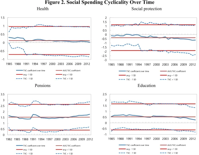
We first report the average level and the time path of the coefficient of social spending cyclicality estimated in equation (2) and (3) for a sample of at most 46 developing countries for which we have time-varying estimates for at least 20 years (Figure 2). Depending on the social spending category in question, the number and composition of countries may change due to data availability.11_{As a first observation, it is worth noting that the time-average health spending}

cyclicality coefficient is positive (about 0.1), which is consistent with the fact that this type of expenditures in our sample is procyclical. However, based on the one standard deviation confidence bands we cannot reject the null that the response of changes in real health spending to changes real GDP is zero (that is, we get, generally, acyclicality). For social protection spending cyclicality, the time-average coefficient equals -0.4, with fluctuations between -0.6 and 0. The coefficient has becoming more negative over time hinting to some counter-cyclical behaviour but, once again, confidence bands suggest acyclicality in this social spending category. A similar pattern can be observed for education spending cyclicality. It has generally been positive and stable over time, despite some downward trending at the end of the period, in line with Frankel et al. (2013) prediction. Finally, regarding the cyclicality of pensions spending, this is the only category that shows a clear procyclical behaviour and the degree of procyclicality has been increasing since the late 1990s.

11_{For health expenditures we have a sample comprising of 29 countries; for social production expenditures we cover} 23 countries; for pension expenditures we have 35 countries; and, finally, for education expenditures we use data for 28 countries.

(11)

10

Figure 2. Social Spending Cyclicality Over Time

Health Social protection

Pensions Education

Note: the figure displays the time profile of the time-varying coefficient estimates for four different social spending categories and covering countries with at least 20 observations. See footnote 9 for the number of countries in each panel. Confidence bands are shown for both the time-average and time-varying estimates based on plus or minus one standard deviation.

The second observation concerns the country heterogeneity hidden by the time profile previously covered. Figure 3 plots the average time-varying cyclicality for the four different social spending categories (it excludes outliers for better readability). Indeed, there is great variation between average cyclicality estimates with the great majority of developing countries in our sample showing procyclical social spending behaviour. However, yet again, as Frankel et al. (2013) allude to, some countries seem to be graduating away from procyclicality into counter-cyclicality. There does not seem to exist a regional pattern though.

-1 -0.5 0 0.5 1 1.5 1985 1988 1991 1994 1997 2000 2003 2006 2009 2012

TVC coefficient over time AVG TVC coefficient avg - 1 SD avg + 1 SD TVC - 1 SD TVC + 1 SD -3 -2.5 -2 -1.5 -1 -0.5 0 0.5 1 1.5 2 1985 1988 1991 1994 1997 2000 2003 2006 2009 2012

TVC coefficient over time AVG TVC coefficient avg - 1 SD avg + 1 SD TVC - 1 SD TVC + 1 SD 0 0.5 1 1.5 2 2.5 3 3.5 1982 1985 1988 1991 1994 1997 2000 2003 2006 2009 2012

TVC coefficient over time AVG TVC coefficient avg - 1 SD avg + 1 SD TVC - 1 SD TVC + 1 SD -1 -0.5 0 0.5 1 1.5 2 2.5 1985 1988 1991 1994 1997 2000 2003 2006 2009 2012

TVC coefficient over time AVG TVC coefficient avg - 1 SD avg + 1 SD TVC - 1 SD TVC + 1 SD

(12)

11

Figure 3. Average Social Spending Cyclicality by country

Note: extreme outliers were excluded for better visibility.

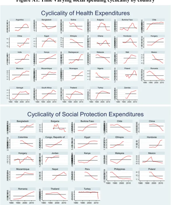
Country specific charts for each social spending category displaying time-varying coefficient estimates are available in Figure A1 in the Appendix. The degree of health spending procyclicality has increased over time for 9 out of 29 countries in the sample. Some, after a period of increasing procyclicality, saw an inversion of the previous trend (e.g. Argentina, Egypt, Senegal, South Africa, Turkey, Mali). Concerning social protection spending procyclicality, several of the set of developing countries covered saw an increase over time (e.g. Bangladesh, Congo, Honduras, Kenya, Romania). In others the degree of procyclicality has stabilized in recent years (e.g. Burkina Faso, Egypt, Mozambique, Philippines, Malaysia). In the case of pensions spending cyclicality, several countries experienced a decline in the degree of its procyclicality since the early to mid-1990s (e.g. Bangladesh, Brazil, Colombia, Mexico, Pakistan, Uganda). In contrast, countries like Chile or Tanzania, the rise in procyclicality over time has been the norm. Finally, when it comes to education spending cyclicality, we also have a heterogeneous picture: countries like Bolivia, Bulgaria, Honduras or Mexico, have seen their degree of procyclicality declining over time; in contrast, Colombia, Indonesia, Romania or Senegal, saw the opposite movement.

Next, we will present and discuss our results from estimating equation (4).

-6 -5 -4 -3 -2 -1 0 1 2 N ic ar ag ua H u ng ar y H o nd u ra s M al i B an gl ad es h So ut h A fr ic a Za m bi a B ur ki n a Fa so Ch in a M al ay si a Eg yp t M o za m bi qu e Tu rk ey In d ia Ch ile Se n eg al Th ai la nd R om an ia Et hi op ia A rg en ti na M o ro cc o Po la nd M ex ic o Ke n ya B ul ga ri a M ad ag as ca r N ig er ia G ha na

Cyclicality of Health Expenditures

-6 -4 -2 0 2 4 6 Ke n ya Ph ili pp in es Tu rk ey B ur ki na F as o Pe ru Po la nd Th ai la nd Ch in a Ch ile M o za m bi qu e R om an ia M al ay si a H u ng ar y Bu lg ar ia Jo rd an Et hi op ia Co ng o, R ep ub lic o f H o nd u ra s M ex ic o Co lo m bi a N ep al Eg yp t

Cyclicality of Social Protection Expenditures

-5 -3 -1 1 3 5 7 Ta nz an ia G ha na In d on es ia Pe ru Co te d 'Iv oi re Eg yp t M ad ag as ca r In d ia B ur ki n a Fa so Pa ki st an M o ro cc o Ch ile A rg en ti na H u ng ar y Se n eg al Tu rk ey Et hi op ia Ph ili pp in es Ke n ya B ol iv ia B ul ga ri a U kr ai ne Za m bi a Ca m er oo n Po la nd M ex ic o Co lo m b ia R om an ia B ra zi l M al ay si a N ig er ia Sa u di A ra b ia Ch in a

Cyclicality of Pension Expenditures

-6 -5 -4 -3 -2 -1 0 1 2 3 N ic ar ag ua N ep al Za m bi a M oz am bi qu e Bu rk in a Fa so Ho nd ur as Eg yp t Ha iti M or oc co Ch ile Ro m an ia So ut h Af ric a Th ai la nd M al i Tu rk ey Se ne ga l In do ne si a Jo rd an Co lo m bi a Bu lg ar ia M ad ag as ca r Et hi op ia Ph ili pp in es M ex ic o N ig er ia Bo liv ia Ke ny a G ha na

(13)

12

4.2 Empirical Findings: Determinants of Social Spending Cyclicality

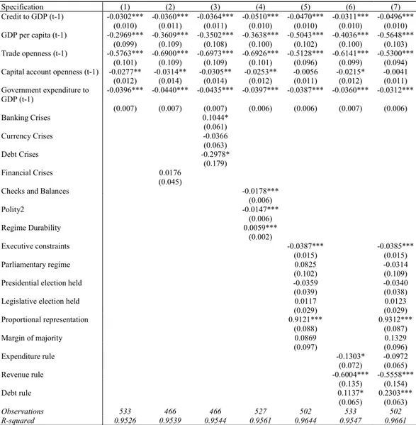
Table 1 presents the results obtained by estimating equation (4) for the case of health spending using different econometric specifications. The coefficients associated with the various determinants typically exhibit the expected sign and confirm the conjectures discussed above. Starting with the set of macroeconomic variables, we find that social spending cyclicality is robustly and negatively associated with the level of financial development, with an increase of 10 percentage points in the credit-to-GDP ratio decreasing the degree of health procyclicality by about 0.3-0.5 (i.e. by about 0.2-0.3 standard deviation). We also find that more developed and open to trade developing economies tend to have a smaller degree of health procyclicality. Similarly, developing countries with larger government are also able to provide more stabilization through increased health spending: an increase of 10 percentage points in the government expenditure-to-GDP ratio decreases health procyclicality 0.3-0.4. Finally, we find that health procyclicality does not generally increase during financial crises once other macroeconomic variables are controlled for but the result depends on the exact type of crisis under consideration (see column 3). Our results suggest that health procyclicality increases during banking crises but declines during sovereign debt crises. Looking at the political variables, we find that constraints on the executive are robustly negatively and significantly associated with health procyclicality. The results are consistent with the evidence provided in Fatas and Mihov (2013) and Lane (2003), who find that more constraints on the executive tend to reduce government spending volatility and positively influence the overall role of fiscal policy stabilization. A similar effect is obtained by better institutional quality, as proxied by either polity 2 or checks and balances. Regime durability, however, seems to be positively correlated with health procyclicality, possibly due to the growing influence of lobbies and other pressure groups next to politicians. Finally, the presence of expenditure and revenue rules seems to reduce the degree of health procyclicality in developing countries.

(14)

13

Table 1. The determinants of health spending cyclicality (WLS)

Specification (1) (2) (3) (4) (5) (6) (7) Credit to GDP (t-1) -0.0302*** -0.0360*** -0.0364*** -0.0510*** -0.0470*** -0.0311*** -0.0496*** (0.010) (0.011) (0.011) (0.010) (0.010) (0.010) (0.010) GDP per capita (t-1) -0.2969*** -0.3609*** -0.3502*** -0.3638*** -0.5043*** -0.4036*** -0.5648*** (0.099) (0.109) (0.108) (0.100) (0.102) (0.100) (0.103) Trade openness (t-1) -0.5763*** -0.6900*** -0.6973*** -0.6926*** -0.5128*** -0.6141*** -0.5300*** (0.101) (0.109) (0.109) (0.101) (0.096) (0.099) (0.094) Capital account openness (t-1) -0.0277** -0.0314** -0.0305** -0.0253** -0.0056 -0.0215* -0.0041 (0.012) (0.014) (0.014) (0.012) (0.011) (0.012) (0.011) Government expenditure to GDP (t-1) -0.0396*** -0.0440*** -0.0435*** -0.0397*** -0.0387*** -0.0360*** -0.0312*** (0.007) (0.007) (0.007) (0.006) (0.006) (0.007) (0.006) Banking Crises 0.1044* (0.061) Currency Crises -0.0366 (0.063) Debt Crises -0.2978* (0.179) Financial Crises 0.0176 (0.045)

Checks and Balances -0.0178*** (0.006) Polity2 -0.0147*** (0.006) Regime Durability 0.0059*** (0.002) Executive constraints -0.0387*** -0.0385*** (0.015) (0.015) Parliamentary regime 0.0825 -0.0314 (0.102) (0.109) Presidential election held -0.0359 -0.0340 (0.039) (0.038) Legislative election held 0.0117 0.0123 (0.029) (0.029) Proportional representation 0.9121*** 0.9312*** (0.088) (0.087) Margin of majority 0.0869 0.1329 (0.097) (0.096) Expenditure rule -0.1303* -0.0972 (0.072) (0.065) Revenue rule -0.6004*** -0.5558*** (0.135) (0.154) Debt rule 0.1137* 0.2303*** (0.065) (0.063) Observations 533 466 466 527 502 533 502 R-squared 0.9526 0.9539 0.9544 0.9561 0.9644 0.9547 0.9661

Note: Results obtained by estimating equation (4). Robust standard errors clustered at the country level in parentheses. Country and time fixed effects were estimated but omitted for reasons of parsimony. The constant term was also omitted for reasons of parsimony. ***, **, * denote significance at 1, 5 and 10 percent level, respectively.

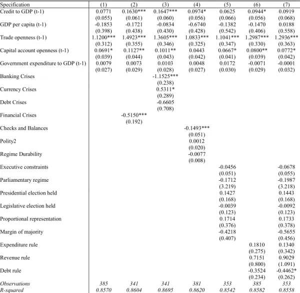
At the same time, some of these determinants tend to have different effects depending on the social spending category under scrutiny. For example, turning to Table 2 – that looks at social protection - here the level of financial deepening, trade and capital account openness are positively associated with its procyclicality. The level of economic development does not seem important in this case to explain social protection cyclicality movements. Financial crises, however, contribute to mitigate the degree of social protection procyclicality. Moreover, with the exception of checks and balances (which has the a priori expected sign), none of the institutional and political economy variables seem to matter.

(15)

14

Table 2. The determinants of social protection spending cyclicality (WLS)

Specification (1) (2) (3) (4) (5) (6) (7) Credit to GDP (t-1) 0.0771 0.1630*** 0.1647*** 0.0974* 0.0625 0.0944* 0.0919 (0.055) (0.061) (0.060) (0.056) (0.066) (0.056) (0.068) GDP per capita (t-1) -0.1853 -0.1721 -0.0834 -0.6740 -0.1382 -0.1470 0.0188 (0.398) (0.438) (0.430) (0.428) (0.542) (0.406) (0.558) Trade openness (t-1) 1.1200*** 1.4923*** 1.3605*** 1.0833*** 1.1041*** 1.2987*** 1.2936*** (0.312) (0.355) (0.346) (0.325) (0.347) (0.330) (0.363) Capital account openness (t-1) 0.0691* 0.1127** 0.1011** 0.0443 0.0667* 0.0800** 0.0772* (0.039) (0.044) (0.043) (0.042) (0.041) (0.039) (0.042) Government expenditure to GDP (t-1) 0.0079 0.0073 0.0103 0.0048 0.0172 -0.0071 -0.0001 (0.027) (0.029) (0.028) (0.027) (0.030) (0.029) (0.032) Banking Crises -1.1525*** (0.238) Currency Crises 0.5311* (0.289) Debt Crises -0.6605 (0.708) Financial Crises -0.5150*** (0.192)

Checks and Balances -0.1493*** (0.051) Polity2 0.0012 (0.020) Regime Durability -0.0077 (0.008) Executive constraints -0.0456 -0.0678 (0.051) (0.055) Parliamentary regime -0.1712 -0.1987 (3.219) (3.218) Presidential election held 0.1427 0.1443 (0.168) (0.168) Legislative election held -0.0039 -0.0092 (0.123) (0.123) Proportional representation 0.1714 0.1733 (0.376) (0.378) Margin of majority -0.4218 -0.5655 (0.407) (0.456) Expenditure rule 0.1810 0.1340 (0.275) (0.342) Revenue rule 0.7151 0.9029 (0.800) (1.091) Debt rule -0.3524 -0.4462* (0.234) (0.262) Observations 385 341 341 381 353 385 353 R-squared 0.8570 0.8604 0.8695 0.8620 0.8542 0.8582 0.8558

Turning to pensions, its degree of procyclicality is positively and significantly affected by the size of the government and degree of capital account openness. As in the case of health spending, the level of financial deepening, economic development and trade openness, all contribute to lower the procyclicality of pensions expenditures. As far as political variables are concerned, having a parliamentary regime with large margins of majority is preferable if one is concerned about boosting the stabilization role of public expenditure policy.

(16)

15

Table 3. The determinants of pensions spending cyclicality (WLS)

Specification (1) (2) (3) (4) (5) (6) (7) Credit to GDP (t-1) -0.0129*** -0.0109*** -0.0106*** -0.0123*** -0.0133*** -0.0076* -0.0092** (0.004) (0.004) (0.004) (0.004) (0.004) (0.004) (0.005) GDP per capita (t-1) -0.2732*** -0.2663*** -0.2687*** -0.2278*** -0.1923** -0.3075*** -0.2359*** (0.068) (0.072) (0.072) (0.073) (0.081) (0.068) (0.082) Trade openness (t-1) -0.2517*** -0.2654*** -0.2662*** -0.2549*** -0.2751*** -0.2474*** -0.2608*** (0.057) (0.059) (0.060) (0.057) (0.060) (0.056) (0.060) Capital account openness (t-1) 0.0235*** 0.0301*** 0.0301*** 0.0254*** 0.0250*** 0.0299*** 0.0300***

(0.008) (0.008) (0.008) (0.008) (0.008) (0.008) (0.008) Government expenditure to GDP (t-1) 0.0094** 0.0078* 0.0076* 0.0104** 0.0144*** 0.0053 0.0101** (0.004) (0.004) (0.004) (0.004) (0.005) (0.004) (0.005) Banking Crises -0.0202 (0.034) Currency Crises -0.0023 (0.035) Debt Crises -0.0188 (0.064) Financial Crises -0.0244 (0.025)

Checks and Balances 0.0042 (0.005) Polity2 -0.0034 (0.004) Regime Durability -0.0015 (0.002) Executive constraints -0.0130 -0.0059 (0.012) (0.012) Parliamentary regime -0.4288*** -0.3445*** (0.095) (0.097) Presidential election held 0.0251 0.0292 (0.027) (0.027) Legislative election held -0.0171 -0.0177 (0.020) (0.020) Proportional representation -0.0325 -0.0655 (0.046) (0.046) Margin of majority -0.1249* -0.1270* (0.071) (0.070) Expenditure rule -0.0953** -0.0712 (0.045) (0.045) Revenue rule -0.1231 -0.1785 (0.174) (0.228) Debt rule -0.1487*** -0.1136*** (0.033) (0.035) Observations 702 628 628 694 610 702 610 R-squared 0.9643 0.9676 0.9676 0.9657 0.9610 0.9660 0.9621

Finally, with regard to education spending cyclicality determinants, we still obtain - as in the case of health - negative and statistically significant coefficients on the level of financial deepening, trade and capital account openness and government size. However, in contrast, the level of development appears to be positively correlated with this social category’s procyclicality. This seems at odds with previous evidence (Talvi and Vegh and Mpatswe et al., 2011) whose prediction was that as nations develop and become richer, their fiscal policies become more stabilizing (of counter-cyclical). None of the institutional or political determinants seem to matter much in this case.

(17)

16

Table 4. The determinants of education spending cyclicality (WLS)

Specification (1) (2) (3) (4) (5) (6) (7) Credit to GDP (t-1) -0.0690*** -0.0659*** -0.0653*** -0.0648*** -0.0846*** -0.0677*** -0.0769*** (0.017) (0.018) (0.018) (0.018) (0.023) (0.018) (0.024) GDP per capita (t-1) 0.4120** 0.3145* 0.3017* 0.5106*** 0.6182*** 0.3804** 0.6632*** (0.167) (0.177) (0.177) (0.173) (0.215) (0.170) (0.221) Trade openness (t-1) -0.8069*** -0.8504*** -0.8704*** -0.8241*** -1.2200*** -0.7430*** -1.1633*** (0.202) (0.212) (0.212) (0.206) (0.220) (0.206) (0.226) Capital account openness (t-1) -0.0477** -0.0655** -0.0660** -0.0457* -0.0594** -0.0445* -0.0532*

(0.024) (0.026) (0.026) (0.025) (0.026) (0.025) (0.028) Government expenditure to GDP (t-1) -0.0880*** -0.0808*** -0.0805*** -0.0883*** -0.0973*** -0.0864*** -0.0947*** (0.008) (0.009) (0.009) (0.009) (0.010) (0.009) (0.010) Banking Crises -0.2267* (0.119) Currency Crises 0.0508 (0.110) Debt Crises 0.2505 (0.224) Financial Crises -0.0135 (0.083)

Checks and Balances 0.0055 (0.028) Polity2 0.0009 (0.010) Regime Durability -0.0009 (0.004) Executive constraints 0.0483 0.0346 (0.031) (0.033) Parliamentary regime 0.2549 -0.0957 (0.180) (0.233) Presidential election held 0.0090 0.0028 (0.087) (0.087) Legislative election held 0.0048 0.0041 (0.071) (0.071) Proportional representation 0.1935 0.2286* (0.136) (0.137) Margin of majority 0.3265 0.3258 (0.209) (0.211) Expenditure rule 0.2013 0.2215 (0.198) (0.206) Revenue rule -0.0460 -0.1036 (0.278) (0.370) Debt rule 0.2327* 0.2929* (0.127) (0.154) Observations 524 482 482 519 457 524 457 R-squared 0.8763 0.8773 0.8787 0.8786 0.8827 0.8782 0.8844

As a robustness check, we replicated the results for the full specification represented by column 7 in Tables 1-4, by alternatively excluding country and/or time fixed effects. Results (available upon request) confirm the previous statistical significance of both macroeconomic and political variables.

A key question is then how can social spending counter-cyclicality be enhanced, particularly in developing countries with high debt-to-GDP levels? Our next exercise consists in conditioning countries based on their level of public debt but also on their level of financial development and institutional quality. More specifically, we split countries between those whose country average is above/below the panel’s median values for public-debt-to-GDP ratio, the credit-to-GDP ratio and polity2, respectively. As before we will focus on the specification represented by column 7 in Tables 1-4. For each social spending category, results conditioned on these three aspects are shown in Appendix Tables A3-A4.

(18)

17

Starting with Appendix Table A3, panel I, we can see that the negative and statistically significant effect of financial deepening, GDP per capita and trade openness are particularly relevant in lowering the degree of health procyclicality in countries highly indebted and characterized by low institutional quality. The beneficial aspect (in a stabilizing sense) of fiscal rules, seems to kick in more strongly in highly indebted countries as well. Constraints on the executive exert a downward force on the degree of health procyclicality in countries with low public debt and poor institutions.

In Appendix Table A3, panel II we observe, in turn, that the more open the economy is, in countries with low debt and poor institutions, the lower the procyclicality of social protection spending. A similar conclusion applies for constraints on the executive as in the case of health.

In Appendix Table A4, panel I we note the fact that higher financial (economic) development exerts a negative influence on pensions spending cyclicality in countries characterized by low debt (financial deepening) and poor institutions. The more open an economy is, the lower the degree of pensions procyclicality in countries with high public debt and financially more developed. Also, debt rules appear to act more strongly (in the sense of lowering procyclicality) in those countries with high public debt, developed financial markets and poor institutions.

Finally, as far as education is concerned, Appendix Table A4, panel II shows that financial deepening reduces education procyclicality in countries with poor institutions. Similarly trade openness has a negative and significant effect of education cyclicality in countries with poor institutions, but also those that are lightly indebted and do not have very developed financial markets. The larger the size of the government the more countercyclical education spending is, particularly in countries with low debt, development financial markets and poor institutions.

The model described above is reduced-form and does not allow making causal statements, meaning that the use of instruments is required.12_{While adding lagged covariates partly corrects}

for these biases, endogeneity can still arise from other omitted variables (unobserved heterogeneity and selection effects), measurement errors in variables and reverse causality (simultaneity). Since causality can run in both directions, some of the right-hand-side regressors may be correlated with the error term. We begin by re-estimating specification 4 of the previous set of tables using a Two Stage Least Squares (TSLS) estimator where instruments are the growth rate of main trading partners and second and third lags of the regressors. In order to account for dynamics, we use a system GMM estimator that exploits stationarity restrictions. This method jointly estimates Equation (4) in first differences, using as instruments lagged levels of the dependent and independent variables, and in levels, using as instruments the first differences of the regressors (Arellano and Bover, 1995; Blundell and Bond, 1998).13 GMM estimators are unbiased, and

compared with ordinary least squares or fixed effects (within-group) estimators, exhibit the

12_{We thank the editor and an anonymous referee for this comment.}

13_{Specifically, we run the two-step system-GMM estimator with Windmeijer standard errors. The significance of the} results is robust to different choices of instruments and predetermined variables.

(19)

18

smallest bias and variance (Arellano and Bond, 1991).14_{We also rely on the Pesaran (2006)}

common correlated effects pooled (CCEP) estimator that accounts for the presence of unobserved common factors by including cross-section averages of the dependent and independent variables in the regression equation, and where the averages are interacted with country-dummies to allow for country-specific parameters. This estimator is a generalization of the fixed effects estimator that allows for the possibility of cross section correlation. Including the (weighted) cross sectional averages of the dependent variable and individual specific regressors is suggested by Pesaran (2006, 2007) as an effective way to filter out the impacts of common factors, which could be common technological shocks or macroeconomic shocks, causing between group error dependence.

Table 5 shows the results of these series of robustness checks. Looking at specifications 1-4 with TSLS we note that the Kleibergen-Paap statistic of weak exogeneity confirms the validity of the instruments used. However, in most specifications we only conservatively reject the null hypothesis that the instrumented variables are exogenous or, in other words, the p-values of the corresponding test statistic are too close or only slightly above 10 percent thus suggesting that the use of instrumental variable estimation may be unwarranted. Moreover, in general most signs and significance levels are retained in comparison with those from Tables 1-4 for the different dependent variables. This is reassuring as a robustness check. Moving on to the dynamic setting with the GMM estimation, the consistency of the obtained set of estimates was checked by using the Hansen and the Arellano-Bond tests. The Hansen test of over-identifying restrictions, which tests the overall validity of the instruments by analysing the sample analog of the moment conditions used in the estimation process, cannot reject the null that the full set of orthogonality conditions is valid. The Arellano-Bond test for autocorrelation cannot reject the null hypothesis of no second-order serial correlation in the first-differenced error terms. Here coefficient estimates generally loose statistical significance, maybe because the system GMM estimator is a very demanding one. Finally, using the CCEP estimator does not reveal any additional insights, as most coefficient estimates turn out to be statistically not different from zero. Then again, conducting Pesaran’s (2004) Cross-Sectional Dependence test (available upon request), we do no reject the null of cross-section independence with a p-value comfortably above the 10 percent level.

14_{As far as information on the choice of lagged levels (differences) used as instruments in the difference (level)} equation, as work by Bowsher (2002) and, more recently, Roodman (2009) have indicated, when it comes to moment conditions (as thus to instruments) more is not always better. The GMM estimators are likely to suffer from “overfitting bias” once the number of instruments approaches (or exceeds) the number of groups/countries (as a simple rule of thumb). In the present case, the validity of instruments was examined using Sargan’s test of overidentifying restrictions. Intuitively, the system GMM estimator does not rely exclusively on the first-differenced equations but exploits also information contained in the original equations in levels.

(20)

Table 5. The determinants of cyclicality: Robustness to alternative estimators

Dependent Cyclicality Variable health Social protection pensions education health Social protection pensions education health Social protection pensions education

Estimator IV IV IV IV SYS-GMM SYS-GMM SYS-GMM SYS-GMM CCEP CCEP CCEP CCEP

Specification (1) (2) (3) (4) (5) (6) (7) (7) (8) 9) (10) (11) Credit to GDP (t-1) -0.2386*** 0.8849*** 0.0149 -0.3012*** -0.0354** -0.0403 -0.0109 -0.0042 -0.0207 0.2188 -0.0545* -0.0939 (0.055) (0.138) (0.057) (0.030) (0.014) (0.110) (0.017) (0.038) (0.122) (0.348) (0.034) (0.070) GDP per capita (t-1) -0.0244 -0.9360*** 0.0443 0.2553*** -0.1983 -0.2198 -0.3148** -0.3232 -0.3054 0.1513 0.3364 -0.5703 (0.075) (0.169) (0.094) (0.045) (0.162) (0.837) (0.148) (0.353) (0.324) (0.891) (0.322) (0.588) Trade openness (t-1) 0.4174 1.6195*** -2.0171*** -1.5421*** -0.0280 -0.1754 -0.0594 0.3138 -0.0178 -0.9799 0.1554 0.1700 (0.287) (0.562) (0.516) (0.386) (0.092) (0.695) (0.106) (0.195) (0.061) (0.801) (0.173) (0.128) Capital account openness (t-1) -0.6053*** 0.7694*** 0.1084 -0.3814*** -0.0122 0.0326 -0.0098 -0.0069 0.0056 0.2474* -0.1015 0.0240 (0.084) (0.179) (0.132) (0.067) (0.026) (0.058) (0.020) (0.062) (0.020) (0.142) (0.080) (0.041) Government expenditure to GDP (t-1) -0.0462* 0.1957*** 0.1411*** -0.0150 -0.0064 -0.0442 -0.0010 -0.0198 -0.0029 -0.0271 0.0291 -0.0025 (0.026) (0.057) (0.043) (0.018) (0.014) (0.039) (0.008) (0.018) (0.005) (0.047) (0.033) (0.017) Checks and Balances 0.0063 0.3418 0.0466 -0.0691 -0.0006 -0.0352 -0.0265*** 0.0014 1.5231 0.1494 0.0088 -0.2929 (0.059) (0.217) (0.103) (0.075) (0.011) (0.065) (0.008) (0.026) (1.061) (0.181) (0.087) (0.316) Polity2 -0.1221*** -0.0965* -0.1459*** -0.0024 -0.0226** 0.0451 0.0029 0.0230* -0.2106 -0.0954 0.0430 0.0157 (0.025) (0.053) (0.036) (0.019) (0.008) (0.044) (0.003) (0.013) (0.170) (0.063) (0.038) (0.034) Regime Durability 0.0312*** 0.0983*** -0.0329*** -0.0263*** 0.0003 0.0173 -0.0042* -0.0056 0.0056 -0.1589 -0.0075 -0.0027 (0.009) (0.019) (0.013) (0.007) (0.003) (0.021) (0.002) (0.004) (0.013) (0.111) (0.015) (0.016) Observations 521 384 692 497 505 381 692 497 527 391 713 513 R-squared 0.1952 0.2267 0.0926 0.2359 0.9997 0.9861 0.9947 0.9977

Kleibergen-Paap test (p-value) 0.01 0.00 0.02 0.04

Wu-Hausman test of endogeneity (p-value)

0.09 0.12 0.10 0.08

ar1 (p-value) 0.000 0.000 0.000 0.000

ar2 (p-value) 0.512 0.481 0.322 0.127

Sargan/Hansen test of overidentifying restrictions (p-value)

0.81 0.29 0.87 0.23

Note: Results obtained by estimating equation (4) with IV (TSLS), system GMM and CCEP estimators. Standard errors in parentheses. Country and time fixed effects were estimated but omitted for reasons of parsimony. The constant term was also omitted for reasons of parsimony. The Kleibergen-Paap rk Wald F statistic of weak exogeneity tests the validity of the instruments used. The Wu-Hausman Test of endogeneity tests the null hypothesis that the regressors are exogenous. Sargan/Hansen test of overidentifying restrictions tests the overall validity of the instruments by analyzing the sample analog of the moment conditions used in the estimation process. The Arellano-Bond tests (ar1 and ar2) evaluate first and second order serial correlation in the error terms. ***, **, * denote significance at 1, 5 and 10 percent level, respectively.

(21)

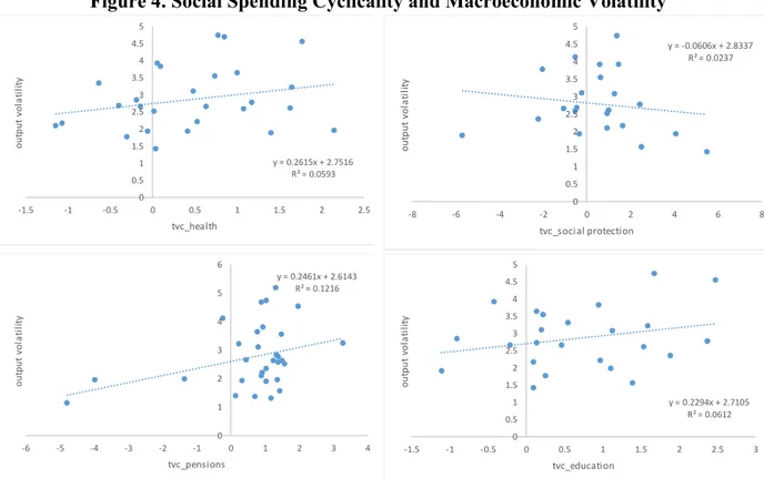
Finally, future research should inspect the consequences of social spending procyclicality to macroeconomic stability. As a teaser, a simple bivariate unconditional scatterplot of each social category cyclicality and a measure of output volatility (proxied by the rolling standard deviation of real GDP growth) is shown in Figure 4. It illustrates the general point that the higher the degree of social spending procyclicality (particularly when it comes to pensions expenditures), the higher the macroeconomic volatility associated. Hence, despite this being an association (and not a causation), there are merits in graduating away from procyclical fiscal policy. Indeed, several studies seem to agree that a timely counter-cyclical response of fiscal policy to (demand) shocks is likely to deliver considerably lower output and consumption volatility (see e.g. Debrun and Kapoor, 2011; Fatas and Mihov, 2012).

Figure 4. Social Spending Cyclicality and Macroeconomic Volatility

Note: the figure displays the correlation between each social spending category average time-varying coefficient estimates and the average rolling standard deviation of real GDP growth. Using the output gap instead does not qualitatively alter our results. The fitted line, regression equation and R-squared are displayed for completeness.

5. Conclusion

Fiscal policy can influence medium-term growth through its support to macroeconomic stability. Most research on fiscal policy cyclicality has, for a long time, focused on advanced economies due to data availability and quality reasons. In this paper we focused on a sample of 45 developing countries and went more granular into the expenditure components of government’s social policy. Using time-varying estimates of social spending cyclicality, we first provided a novel

y = 0.2615x + 2.7516 R² = 0.0593 0 0.5 1 1.5 2 2.5 3 3.5 4 4.5 5 -1.5 -1 -0.5 0 0.5 1 1.5 2 2.5 ou tp ut v ol at ili ty tvc_health y = -0.0606x + 2.8337 R² = 0.0237 0 0.5 1 1.5 2 2.5 3 3.5 4 4.5 5 -8 -6 -4 -2 0 2 4 6 8 ou tp ut v ol at il ity tvc_social protection y = 0.2461x + 2.6143 R² = 0.1216 0 1 2 3 4 5 6 -6 -5 -4 -3 -2 -1 0 1 2 3 4 ou tp ut v ol at ili ty tvc_pensions y = 0.2294x + 2.7105 R² = 0.0612 0 0.5 1 1.5 2 2.5 3 3.5 4 4.5 5 -1.5 -1 -0.5 0 0.5 1 1.5 2 2.5 3 ou tp ut v ol at ili ty tvc_education

(22)

21

characterization of its behaviour across countries and over time and then we went on to empirically inspect its main macroeconomic and institutional determinants.

At the aggregate average, we found that, with the exception of spending on pensions which has been procyclical over time, the other social spending components have generally been acyclical in developing countries. However, sample averages hide high degrees of heterogeneity between countries. The great majority of developing countries in our sample displayed procyclical social spending behaviour. However, as Frankel et al. (2013) allude to, some countries seem to be graduating away from procyclicality into counter-cyclicality but no clear regional pattern seems to exist.

Moreover, while a large body of the literature has typically found that government size is the main determinant of the stabilizing role of government spending policies, the results presented in this paper suggest that other macroeconomic policies and institutional and political characteristics can also affect the degree of social spending cyclicality for a given government size. In particular, while some drivers affect different social components’ cyclicality differently, in general, our results suggest that in addition to political constraints, policies aimed at fostering financial deepening, the level of economic institutions and trade openness can significantly reduce the degree of procyclicality of social spending. Moreover, fiscal rules seem to be important in curbing the procyclical behaviour of social spending. That being said, some results are conditional on whether countries are characterized by high or low levels of public indebtedness and if they operate under developed financial markets and strong institutions, or not.

Future research on the topic should consider looking at the consequences of procyclical social policy, since as we briefly demonstrated – using unconditional associations -, the larger the degree of procyclicality, the higher the macroeconomic instability (which compromises growth prospects).

(23)

Conflict of Interest Disclosure

(24)

23 References

1. Abbott, R. Cabral, P. Jones, R. Palacios (2015), “Political pressure and procyclical expenditure: An analysis of the expenditures of state governments in Mexico”, European Journal of Political Economy, 37, 195-206

2. Abdih, Y., Lopez Murphy, P., Roitman, A., Sahay, R. (2010), “The cyclicality of fiscal policy in the Middle East and Central Asia: is the current crisis different?”, IMF WP Series No. 10/68.

3. Acemoglu, D., S. Naidu, P. Restrepo, and J. A. Robinson (2013), “Democracy Does Cause Growth”, NBER Working Paper 20004.

4. Afonso, A., and J. T. Jalles. (2013), “The Cyclicality of Education, Health, and Social Security Government Spending”, Applied Economics Letters 20 (7), 669–72.

5. Aghion, P. and I. Marinescu (2008), “Cyclical Budgetary Policy and Economic Growth: What Do We Learn from OECD Panel Data?”, NBER Macroeconomics Annual, Volume 22

6. Alesina, A., Campante, F.R., Tabellini G.R. (2008), “Why Is Fiscal Policy Often Procyclical?” Journal of the European Economic Association. 6(5), 1006-103

7. Arellano, M., & Bover, O. (1995), “Another look at the instrumental variable estimation of error-components models”. Journal of Econometrics, 68(1), 29–51.

8. Arellano, M., and Bond, S. (1991), “Some Tests of Specification for Panel Data: Monte Carlo Evidence and an Application to Employment Equations”. The Review of Economic Studies, 58(2), 277.

9. Barro, R. J. (1979), “On the determination of the public debt”, Journal of Political Economy, 87, 940–971. 10. Blundell, R., & Bond, S. (1998), “Initial conditions and moment restrictions in dynamic panel data models”. Journal of Econometrics, 87(1), 115–143.

11. Bowsher, C. G. (2002), “On testing overidentifying restrictions in dynamic panel data models”. Economics Letters, 77(2), 211–220.

12. Braun, M., and L. Di Gresia (2003), “Towards Effective Social Insurance in Latin America: The Importance of Countercyclical Fiscal Policy.” Inter-American Development Bank Working Paper 487, Washington, DC. 13. Calderón, C. and K. Schmidt-Hebbel. (2008), “Business Cycles and Fiscal Policies: The Role of Institutions and Financial Markets”, Central Bank of Chile Working Paper Nº 481, August.

14. Debrun, X. and R. Kapoor (2011), “Fiscal Policy and Macroeconomic Stability: New Evidence and Policy Implications”, Nordic Economic Policy Review, 1(1), 35-70.

15. Debrun, X., Pisani-Ferry, J., Sapir, A. (2008), “Government Size and Output Volatility: Should We Forsake Automatic Stabilization?”, International Monetary Fund, IMF Working Paper 08/122, May 2008.

16. Diallo, O. (2009), “Tortuous Road Toward Countercyclical Fiscal Policy: Lessons from Democratized Sub-Saharan Africa,” Journal of Policy Modelling, 31,36–50.

17. Doytch, N., B. Hu, and R. U. Mendoza (2010), “Social Spending, Fiscal Space, and Governance: An Analysis of Patterns over the Business Cycle.” UNICEF Policy and Practice, second draft, April.

18. Drazen, A. (2000), “The Political Business Cycle after 25 Years.” In: B. Bernanke and K. Rogoff, eds. NBER Macroeconomics Annual 2000. Cambridge, MA: MIT Press.

19. Egert, B. (2012), “Fiscal Policy Reaction to the Cycle in the OECD: Pro-or Counter-cyclical”, CEsifo working papers, 3777.

20. Fatas, A. and I. Mihov (2012), “Fiscal policy as a stabilization tool”, B.E. Journal of Macroeconomics, 12(3), 1-68.

21. Fatas, A. and I. Mihov (2013), “Policy Volatility, Institutions, and Economic Growth”, Review of Economics and Statistics 95: 362-376.,

22. Frankel, J., C. Vegh and G. Vuletin (2011), “On graduation from fiscal procyclicality,” NBER Working Paper No. 17619 (November).

23. Furceri, D. (2010), “Stabilization effects of social spending: Empirical evidence from a panel of OECD countries”, North American Journal of Economics and Finance, 21(1), 34-48.

24. Galí, J. (1994), “Government Size and Macroeconomic Stability”, European Economic Review 38: 117–32 25. Gavin, M., and R. Perotti (1997), “Fiscal Policy in Latin America.” NBER Macroeconomics Annual 1997, edited by Ben Bernanke and Julio Rotemberg. MIT Press

26. Gavin, M., Hausmann, R., Perotti, R., and Talvi, E. (1996), “Managing Fiscal Policy in Latin America and the Caribbean: Volatility, Procyclicality, and Limited Creditworthiness”, mimeo, Office of the Chief Economist, InterAmerican Development Bank.

27. Granado, J., Gupta, S., Hajdenberg, A. (2013), “Is Social Spending Procyclical? Evidence for Developing Countries”, World Development, 42, 16-27.

(25)

24

28. Ilzetzki, E., Vegh, C. (2008), “Procyclical fiscal policy in Developing Countries: truth or fiction?”, NBER WP No. 14191.

29. IMF (2015). World Economic Outlook, October.

30. Kaminsky, G., C. Reinhart, and C. Végh, (2004), “When it Rains, it Pours: Procyclical Capital Flows and Macro Policies,” NBER Macroeconomics Annual 2004, edited by Mark Gertler and Kenneth Rogoff, 19: 54-61. Cambridge, MA: M.I.T. Press.

31. Laeven, L. and Valencia F., (2010), “Resolution of Banking Crises: The Good, the Bad, and the Ugly.” International Monetary Fund Working Paper No. 10/146

32. Lane, P. R. (1998), “On the Cyclicality of Irish Fiscal Policy,” Economic and Social Review, 29(1), 1–17. 33. Lane, P. R. (2003), “The Cyclical Behaviour of Fiscal Policy: Evidence from the OECD”, Journal of Public Economics, 87(12), 2661–2675.

34. Molina, C. (2003), “Gasto Social en America Latina,” Technical Report I-37, Interamerican Development Bank.

35. Mpatswe, G. K., Tapsoba, S. J.-A., and York, R. C. (2011), “The Cyclicality of Fiscal Policies in the CEMAC Region”. IMF Working Papers WP/11/205.

36. Neumeyer, Pablo A., and Fabrizio Perri (2005), “Business Cycles in Emerging Economies: The Role of Interest Rates,” Journal of Monetary Economics, 52(2), 345–380.

37. Persson, T. and G. Tabellini (2000), “Political Economics: Explaining Economic Policy”, Cambridge, MA: MIT Press

38. Pesaran, M. H. (2004), “General Diagnostic Tests for Cross Section Dependence in Panels.” CESifo Group Munich CESifo Working Paper Series 1229

39. Pesaran, M. H. (2006). Estimation and Inference in Large Heterogeneous Panels with a Multifactor Error Structure. Econometrica, 74(4), 967–1012.

40. Prasad, N. and Gerecke, M. (2010) “Social Security Spending in Times of Crisis”, Global Social Policy, 10(2), 218-247.

41. Real, I. and R. Vicente (2008), “Politica Fiscal y Vulnerabilidad Fiscal en Uruguay, 1976-2006,” Technical Report.

42. Reinhart, C. M., and K. S. Rogoff (2011), “From Financial Crash to Debt Crisis” American Economic Review, 101(5), 1676-1706

43. Rodrik, D. (1998), “Why Do More Open Economies Have Bigger Governments”, Journal of Political Economy, 106, 997-1032.

44. Roodman, D. (2009), “A Note on the Theme of Too Many Instruments”. Oxford Bulletin of Economics and Statistics, 71(1), 135–158.

45. Schlicht, E. (2003). “Estimating time-varying coefficients with the VC program”. Discussion Paper 2003-06. University of Munich

46. Schlicht, E. and Ludsteck, J., (2006), “Variance Estimation in a Random Coefficients Model”, IZA Discussion Papers 2031, Institute for the Study of Labor (IZA).

47. Schlicht, E., (1985), “Isolation and Aggregation in Economics”, Berlin-Heidelberg-New York-Tokyo: Springer-Verlag. 22.

48. Staehr, K. (2008), “Fiscal policies and business cycles in an enlarged Euro Area”, Economic Systems, 32, 46-49.

49. Talvi, E., and C. Vegh. (2005). “Tax Base Variability and Procyclical Fiscal Policy”, Journal of Development Economics, Vol. 78, pp. 156-90.

50. Thornton, J. (2008), “Explaining Pro-Cyclical Fiscal Policy in African Countries,” Journal of African Economies, 17(3), 451–64.

51. Tornell, A., Lane, P. (1999), “The voracity effect”, American Economic Review, 89, 22- 46.

52. Uribe, M. and V. Yue (2006) “Country Spreads and Emerging Countries: Who Drives Whom?”, Journal of International Economics, 6-36.

53. Vegh, C. A., Vuletin, G. (2012), “How is tax policy conducted over the business cycle?”, NBER Working Paper No. 17753.

54. Woo, J. (2009), “Why do more polarized countries run more pro-cyclical fiscal policy?”, Review of Economics and Statistics, 91(4), 850-870.

(26)

25 APPENDIX

Figure A1. Time Varying social spending cyclicality by country

.8 5 0 8.8 5 1.8 5 1 2.8 5 1 4 -. 4-. 3 9 9 5-.3 99-.3 9 8 5 -9 .7 4 9 4 -9 .7 4 9 2 -9 .7 4 9 -9 .7 4 88 1 .6 2 8 2 1 .6 2 8 2 5 1 .6 2 8 3 1 .6 2 8 35 -. 1 4 2 5 -. 1 4 2 4 8 -. 1 4 2 4 6 -. 1 4 2 4 4 -. 1 4 2 42 .4 8 4 4 5 .4 8 4 5 .4 8 4 5 5 .4 8 4 6 .4 8 4 6 5 -. 5 0 .5 -2 -1 0 1 .4 .6 .8 1 1 .2 2 .1 4 7 2 2 .1 4 7 2 5 2 .1 4 7 3 2 .1 4 7 3 5 -1 .0 6 7 9 -1 .0 6 7 8 5 -1 .0 6 7 8 -1 .0 6 7 7 5 -1 .0 6 7 7 -1 .1 4 5 -1 .1 4 4 -1 .1 4 3 -1 .1 4 2 .4 1 9 9 5.4 2.4 2 0 0 5 .4 2 0 1 1 .4 0 2 6 1 .4 0 2 7 1 .4 0 2 8 1 .4 0 2 9 1 .4 0 3 1 .6 4 1 8 1 .6 4 1 8 5 1 .6 4 1 9 1 .6 4 1 95 .0 1 5 1 .0 1 5 2 .0 15 3 .0 1 5 4 .0 1 5 5 -. 6 3 5 5 -. 6 3 5 -. 6 3 4 5 -. 6 3 4 -. 6 3 3 5 .5 1 1 .5 2 0 .5 1 1 .5 2 .0 5 6 7 5 .0 5 6 8 .0 5 6 8 5 .0 5 6 9 .0 5 6 9 5 -5 .7 1 5 7 -5 .7 1 5 6 -5 .7 1 5 5 -5 .7 1 5 4 -5 .7 1 5 3 1 2 3 4 1 .0 7 6 1 2 1 .0 7 6 1 4 1 .0 7 6 1 6 1 .0 7 6 1 8 .7 3 7 4.7 3 7 6.7 3 7 8.7 3 8 -1 0 1 2 -. 3 0 6 6 -. 3 0 6 5 -. 3 0 6 4 -. 3 0 6 3 .6 3 3 5 5.6 3 3 6.6 3 3 6 5 .0 9 7.0 9 8.0 9 9 .1 -. 1 9 3 4 -. 1 9 3 2 -. 1 9 3 -. 1 9 2 8 -. 1 9 2 6 1980 1990 2000 2010 1980 1990 2000 2010 1980 1990 2000 2010 1980 1990 2000 2010 1980 1990 2000 2010 1980 1990 2000 2010

Argentina Bangladesh Bolivia Bulgaria Burkina Faso Chile

China Egypt Ethiopia Ghana Honduras Hungary

India Kenya Madagascar Malaysia Mali Mexico

Morocco Mozambique Nicaragua Nigeria Poland Romania

Senegal South Africa Thailand Turkey Zambia

newtime

Cyclicality of Health Expenditures

-1 8. 35 9 -1 8. 35 8 -1 8. 35 7 -1 8. 35 6 -2 0 2 4 -1 .0 6 -1 .0 58 -1 .0 56 -1 .0 54 -. 23 55 5 -. 23 55 -. 23 54 5 -. 23 54 -. 23 53 5 -. 33 55-. 33 5-.3 34 5 2. 50 96 2. 50 982. 512. 51 02 1. 45 2 1. 45 3 1. 45 4 1. 45 5 5. 49 25. 49 45. 49 6 1. 37 1 1. 37 2 1. 37 3 1. 37 4 11 .5 22 .5 3 -1 0 1 2 3 1. 26 18 5 1. 26 191.2 61 95 -5 .6 94 9 -5 .6 94 8 -5 .6 94 7 -5 .6 94 6 -5 .6 94 5 .8 8.9 .9 2.9 4.9 6 0 2 4 6 8 .5 88 .5 9.5 92. 59 4 33 .5 44 .5 5 -. 56-. 55-. 54-. 53-. 52 -2 .2 15 8 -2 .2 15 6 -2 .2 15 4 -1 -. 5 0 .6 35 6.6 35 8.6 36 -. 45 33 -. 45 32 -. 45 31-.4 53-.4 52 9 -6 0-40 -2 0 0 1980 1990 2000 2010 1980 1990 2000 2010 1980 1990 2000 2010 1980 1990 2000 2010 1980 1990 2000 2010

Bangladesh Bulgaria Burkina Faso Chile China

Colombia Congo, Republic of Egypt Ethiopia Honduras

Hungary Jordan Kenya Malaysia Mexico

Mozambique Nepal Peru Philippines Poland

Romania Thailand Turkey

newtime