FUNDAÇÃO GETÚLIO VARGAS
ESCOLA DE ECONOMIA DE EMPRESAS DE SÃO PAULO
Gilberto Orestis Picareta Giannakopoulos
FUNDAÇÃO GETÚLIO VARGAS
ESCOLA DE ECONOMIA DE EMPRESAS DE SÃO PAULO
Gilberto Orestis Picareta Giannakopoulos
Effects of Capital Structure on Markups and Competitive Performance Evidence from Portugal
SÃO PAULO 2016
Dissertação apresentada à Escola de Economia de Empresas de São Paulo da Fundação Getúlio Vargas, como requisito para obtenção do título de Mestre Profissional em Economia.
Campo do Conhecimento: International Master in Finance
Picareta Giannakopoulos, Gilberto Orestis.
Effects of Capital Structure on Markups and Competitive Performance: Evidence from Portugal / Gilberto Orestis Picareta Giannakopoulos. - 2016. 39 f.
Orientadores: Cláudio Custódio e Marcelo Fernandes
Dissertação (mestrado) - Escola de Economia de São Paulo.
1. Estrutura de capital. 2. Empresas - Lucros - Portugal. 3. Concorrência. 4. Desempenho. 5. Crise econômica. I. Custódio, Cláudio. II. Fernandes Marcelo. III. Dissertação (mestrado) - Escola de Economia de São Paulo. IVI. Título.
Gilberto Orestis Picareta Giannakopoulos
Effects of Capital Structure on Markups and Competitive Performance Evidence from Portugal
Dissertação apresentada à Escola de Economia de Empresas de São Paulo da Fundação Getúlio Vargas, como requisito para obtenção do título de Mestre Profissional em Economia.
Campo do Conhecimento: International Master in Finance
Data de Aprovação: 22/01/2016
Banca Examinadora:
______________________________ Prof. Dr. Cláudia Custodio
______________________________ Prof. Dr. Marcelo Fernandes
Acknowledgements
Before everyone else I would like to thank my father who has always guided me by
example in academia and in all relevant aspects of life. I would also like to thank my
mother for making me question generally accepted truths and showing to me that the
world has to be seen through the eyes of many to be understood. I am thankful for
having a little brother that is the most precious gift that one can have in life. I wish to
thank my parents for having supported my studies financially by paying rent, food,
flight tickets, violin classes, insurance, the repairs for my Renault 4L, my Vespa, and
Surfboards. I would like to thank my grandmother for preparing meals that have fed me
well throughout my time in Portugal. I would like to thank Brazil and its people for
teaching me about positivity. I would like to thank the Portuguese sea for receiving
swell, its beaches for producing good surf, and I am thankful for the few that have
Resumo
Este estudo avalia os efeitos da estrutura de capital nas margens de lucro e no
desempenho competitivo. Aplica teorias relativas à contra ciclicidade das margens de
lucro, e aos resultados do mercado do produto de Chevalier e Scharfstein (1996), a
dados portugueses, seguindo a metodologia de Campello (2001). Utilizando dados de
painel de empresas pertencentes à indústria transformadora Portuguesa, a análise
fornece evidencia para a contra-ciclicidade de margens de lucro e de um efeito conjunto
de dívida e recessão económica nas margens de lucro. Tendo por base o recenseamento
de empresas Portuguesas, a análise não fornece evidência de uma relação significativa
entre a estrutura de capital e o desempenho competitivo.
Abstract
This paper examines the effects of capital structure on markups and competitive
performance. It applies theories of markup counter cyclicality and product market
outcomes by Chevalier and Scharfstein (1996) to Portuguese data following the
methodology from Campello (2001). Using industry level panel data of the Portuguese
manufacturing industry, the analysis provides evidence for markup counter cyclicality
and a joint effect of leverage and economic downturn on markups. Using a firm level
census of Portuguese companies the analysis provides no evidence for a significant
relationship between capital structure and competitive performance.
Table of Contents
Introduction 9
1. Literature Review 10
2. Industry Level Analysis 14
2.1 Data 16
2.2 Results from the industry level analysis and interpretation 21
2.3 Limitations 23
3. Firm Level Analysis 24
3.1Data 25
3.2Analysis 26
3.3 Results from the firm level analysis and interpretation 30
3.4 Limitations 31
4. Conclusions 32
References 35
Appendix 37
A1: The ‘robust’ option in STATA 37
A2: Fixed Effects Regression in STATA 38
A3: Complementary estimates and regression results 39
Introduction
A common way of competition between firms in an industry is price competition. In
more mature industries when products tend to be perceived as a commodity by
consumers, many companies compete on the basis of prices. Firms increase market
share by cutting prices thereby also reducing their markup. Particularly, in times of
crisis a firm’s capital structure can restrict the extent to which a firm can reduce its
markup. During economic downturns tighter covenants and the related cost of debt can
restrict a company’s ability to compete. This paper investigates the effect of capital
structure on competitive behaviour of Portuguese companies. This is analysed at two
levels. First, by looking at the effect of leverage on markups during demand shocks at
the industry level and, second, by analysing competitive performance over the business
cycle at the firm level. 1
A firm in an aggressive competitive environment will reduce markups through the
reduction of prices. The reduction of prices is seen as investment in market share- or
sales growth (Chevalier & Scharfstein, 1996). However, in the case of demand shocks,
for example, during a crisis, a firm might be constrained to decrease prices, as it
requires cash flow to nourish its capital structure (Klemperer, 1995). The expectation is
that a relatively highly leveraged firm will have less ability to reduce markups as its
capital structure requires it to cover costs associated with its debt. Consequently, during
economic downturns the leveraged firm will be unable to compete with predatory
pricing imposed by relatively low-leveraged counterparts. An obstacle in this analysis is
endogeneity caused by a confounding variable implying that capital structure and
behaviour may be influenced by a third variable, which has not been included in the
model because it is unobservable. To overcome this obstacle the paper analyses
performance following events affecting competitors’ ability to compete under their
given capital structure. The event is the systemic 2008 financial crisis, which could not
be previously anticipated by market participants.
Using industry level panel data of the Portuguese manufacturing industry, the analysis
provides evidence for markup counter cyclicality and a joint effect of leverage and
economic downturn on markups. From the firm level census data of Portuguese
companies the no evidence for a significant relationship between capital structure and
competitive performance is derived.
The paper is divided into four sections. Section one introduces the foundations of the
studies of capital structure and provides a literature review on academic research about
the impact of capital structure on competitive performance. The second section presents
data, results, interpretation, and limitations for the industry-level analysis. The third
section has the same structure for the firm-level analysis. In the fourth section
conclusions are summarised, major limitations are presented, and themes for further
research are elaborated.
1. Literature Review
This paper’s goal is to analyse how capital structure influences a firm’s and its
competitors’ behaviour. In business and economics academia much work has been
represents the foundation for research on capital structure. In their scenario of a perfect
capital market, the choice between equity and debt does not matter, since under the
assumption of no transaction- and bankruptcy costs, firm value is unaffected by the
choice of financing (Modigliani & Miller, 1958). The leveraged firm as opposed to the
unleveraged firm has a higher cost of equity due to the financial risk associated with
debt but the total value remains unaffected. This is why in their scenario with taxes an
all-debt capital structure is considered optimal. Moreover, the move from Modigliani
and Miller’s perfect scenario into reality along with its imperfections, made theoretical
and empirical researchers evolve in two different directions.
First, there is the study of the effect of capital structure on relationships of agents inside
the firm. This direction deals with agency cost and has been fundamentally influenced
by Jensen and Meckling’s paper (1976) who describe a value loss from information
asymmetry between management and outside investors in a theoretical framework. An
optimal capital structure can be reached by trading off the cost of debt such as cost of
financial distress and agency cost against the benefit of debt. The benefit of debt is often
associated with the tax shield but debt can also have a disciplining effect on
management (Harris & Raviv, 1990). Furthermore, the static tradeoff- and pecking
order theory have provided theoretical explanations for the importance of choosing
different modes of financing (Myers, 1984). A series of authors empirically tested these
theoretical models and found confirming- and disconfirming evidence creating an
academic dialogue about the applicability of these theories, for example between
The second direction of research concerns the study of the effect of capital structure on
relationships of agents outside a firm. This involves competitors, consumers and the
resulting product market outcomes. The variables analysed are price, costs, and
quantity. A firm’s choice of these variables has been observed to affect competition.
Furthermore, capital structure in turn impacts the equilibrium strategies and payoffs
(Harris & Raviv, 1991). Literature in this line of study adopts the view that managers
are incentivised to maximise equity value rather than profits. There are two main
opposing theories that explain how capital structure influences competitive outcomes.
First, based on Jensen and Meckling’s idea that by taking on more debt equity holders
are induced to take riskier actions, Brander and Lewis’ theory (1986) of strategic
commitment suggests that a relatively highly leveraged firm has an incentive to pursue
strategies that raise returns in good states but lower return in bad states. They argue that
firms with higher leverage cut their prices to attain a higher market share even during
negative demand shocks.
Second, Bolton and Scharfstein (1990) posit that firms with a lot of debt financing have
a disadvantage as opposed to their less leveraged competitors. Competitors with less
financial constraints can draw a firm out of competition by setting extremely low prices.
Contrary to the theory of strategic commitment Bolton and Scharfstein’s predatory
pricing theory implies that particularly in periods of low demand financially constrained
firms can suffer from not being able to keep up with price competition.
Chevalier and Scharfstein (1996) revisit this idea and find that debt-financed firms are
sample from the US American supermarket industry they observe that during periods of
negative demand shocks liquidity-constrained firms boost short-run profits by raising
prices. In this case the increase in prices leads to a loss in market share.
Further, Campello (2001) provides evidence for Chevalier and Scharfstein’s results.
Campello examines a sample from the US manufacturing industry and finds that
relatively high leveraged companies have higher markups during recessions but not
during booms. This implies that during recession firms change their competitive
behaviour due to their capital structure. Further, Campello’s findings show that capital
structure’s impact on competitive behaviour is contingent on the capital structure of
other competitors in the same industry. However, during booms capital structure does
not lead to differentiated behaviour. The evidence for counter cyclicality of markups
(Cheavlier and Scharfstein, 1996; Campello, 2001) is challenged in Nekarda and
Ramey's paper (2013) on cyclical behaviour of the price-cost markup.
From the two directions presented the latter is fairly unexplored. This paper aims to
‘reanimate’ the debate by extending the work of Chevalier and Scharfstein (1996) and
of Campello’s (2001) with an industry-level analysis of the Portuguese manufacturing
industries and a firm-level analysis with a census of Portuguese companies. The
analysis closely follows the theoretical approach from Campello’s paper (2001). It
examines the effect of capital structure on markups to test Bolton and Scharfstein’s
predatory pricing theory (1990). Further, it analyses a firm’s competitive performance
contingent on its capital structure and associated ‘financial fragility’ during demand
Whereas Bolton and Scharfstein (1990) solely used debt to define financial fragility,
this paper opts for Campello’s method (2001) by considering a firm financially fragile
only under three conditions. First, the firm has to be highly leveraged relative to its
industry rivals. Second, it is in a market where debt financing is low.
The contribution of this work is the following. First, the analysis of Campello (2001) is
replicated using a more recent and detailed dataset of companies operating in the
Portuguese manufacturing sector and includes firm level data. Second, the more recent
data captures the period of the financial crisis in Europe, which represents a vastly
stronger negative demand shock than the ones studied in previous research. Third, a
census of all Portuguese companies is used for the firm level analysis, compared to a
sample as in previous work by Campello (2001). This allows for a more accurate
measurement of the effects of capital structure.
2. Industry Level Analysis
In terms of methodology this section replicates Campello’s (2001) industry analysis.
This section aims to test the theory of counter cyclicality of markups brought forward
by Chevalier and Scharfstein (1996). Consequently, the expectation is that during
recessions markups increase. The resulting hypothesis states:
H0: Negative economic activity has no positive effect on markup
HA: Negative economic activity has an effect on markup
It also investigates debt’s effect on cyclicality of markups. Following Bolton and
Scharfstein’s initial theory (1990) there should be a joint effect of debt and recession on
H0: Debt and negative economic activity have no joint positive effect on markup
HA: Debt and negative economic activity have a joint positive effect on markup
The resulting empirical model allows testing for countercyclical markups on the
industry level and for the effect of leverage on markups. The regression involves the
dependent variable markup and the three explanatory variables economic activity,
industry leverage, and the interaction term of economic activity and leverage. The
model is stated in equation 1.
Equation 1: Empirical Model
Markup!,!=!+! −Δlog !"# ! +!!"#"$%&"!,!!!+!!"#"$%&"!,!!!× −Δlog !"# ! +!!,!
The -log(GDP) serves as proxy for decreasing economic activity. A positive alpha
coefficient means that during recession markups increase. Just like in Campello (2001)
leverage is lagged one period. This diminishes the simultaneity between markup and
leverage. The OLS regression uses heteroscedasticity-consistent standard error
estimates to correct against a potential violation of the OLS assumptions. To understand
Campello’s (2001) data and methodology his dataset and results were replicated.
Similar findings were obtained. The methodology was changed in a few aspects to
better fit the context of the Portuguese data but did not have an impact on the qualitative
2.1 Data
As for the data used, the paper generally aims to use similar types of data and variables
as deployed by Campello (2001)2. The panel data ranges from 2004 to 2013 and
includes industry-level data from 22 industries of the Portuguese manufacturing sector
resulting in a total of 198 observations. The industries are classified according to the
Portuguese industry classification ‘Classificação Portuguesa das Actividades
Económicas Rev.3’ (CAE 3.0) and are denoted with the codes 10 to 31. Most data have
been compiled through the database of the ‘Instituto Nacional de Estadística’ (INE), the
national statistics bureau in Portugal. Three primary series have been constructed.
First, the markup series, generally price over cost, is calculated according to Campello’s
(2001) simplified version of Bil’s (1987) definition of markup. One major advantage of
Bil’s measure is that it overstates markup cyclicality less than other common measures
like the one used by Rotemberg and Woodford (1991). It allows the incremental cost of
one hour of labour to change with the level of hours worked in an industry3. One
drawback for Bils’ measure, however, is that productivity shifts over the business cycle
are not reflected. This is due to the fact that it takes gross output over the whole period
thereby calculating only one productivity level and does not show when workers are
more or less efficient during sub periods. Also it does not take into account whether
workers are more or less productive in times of economic downturn or growth.
2 Before analysing Portuguese data Campello’s work (2001) was replicated on his own data. The
regression outputs can found in the appendix 3.
3 Note: The cost of an hour of labour increases if overtime hours have been worked – that is more
Equation 2: Markup
!"#$%&!=ln !! −ln !! −ln(1+rV! !! )−ln
!!!!!! !!
−!"#$%−!"#$%&#%
P price of a product
w hourly average wage
r legal overtime premium
H weekly average hours
V(H) overtime hours
j number of weeks in a period
N number of production workers per industry
Y gross output
Generally, markup is price over marginal cost. As can be seen in Equation 2 the markup
series is calculated with Price P, hourly wage w, weekly average hours H, overtime
hours V(H), the number of weeks in a period j, number of production workers N, the
gross output Y and the variable V’(H). V’(H) equals one when the weekly average
hours of work in the industry exceed 40 hours and zero otherwise.
Most of the data used was retrieved as yearly data. If not – it was converted into yearly
data by taking averages or sums. A general obstacle in the data collection was the
conversion between two CAE formats, namely CAE 2.1 and CAE 3.0. To solve this, the
CAE brochures as well as conversion tables were used to convert all data into the final
classification CAE 3.0 (Instituto Nacional de Estatística, 2003; 2007). In a few cases
availability of data for specific time ranges was lacking, for example, for gross output.
After contacting INE the missing data was provided.
Price P was taken from the INE and is a typical index of output prices that allows for
cross-industry comparison. The output price is the price producers receive from the
account any legal entity operating in that industry. This feature is important later on
when using the INE data together with the census data.
On the cost side, hourly wage w is obtained via the gross wages and salaries in industry
series and the total amount of hours worked series – both obtained from the INE.
Similarly, effective weekly average hours H, and number of production workers N were
taken from the same source for each industry, respectively.
In line with Campello (2001), overtime hours V(H) were derived as the weekly average
hours H that exceed 40. This is not very accurate since overtime hours can be worked
even if the weekly average hours are below 40. For instance, a worker can accumulate
overtime hours on one day before the closing of a big order but still work less than 40
hours in a week. However, as the actual series of overtime hours is not available and
could not be provided by the INE, the former method is adopted.
The gross output Y is obtained from the INE for each industry. Gross output measures
two components. First, it measures an industry’s sales to other industries – the
intermediate inputs. The second component is the sale to final users in the economy,
which represents GDP.
For the overtime premium r, a legal overtime premium of 50% is used for the first hour
of overtime and 75% for the second. This is in line with the Portuguese labour standards
that prevailed in the applicable period (Economias, 2015).
The second series is the leverage series, which is computed as the asset-weighted
average long-term debt-to-asset ratio illustrated in Equation 2. The leverage series is
compiled on the basis of a census of all Portuguese companies operating in the
was obtained via an institution of the INE ‘IES - Informação Empresarial Simplificada’
(Instituto Nacional de Estatistica, 2015). As can be seen in Equation 3 the calculation
includes total assets ‘Total do Activo bruto’ and total long-term debt ‘Total Dividas a
terceiros a médio e longo prazo’.
Equation 3: Leverage
Leverage! = !""#$"! !""#$"! ! !!! ! !!! ∙ !"#$! !""#$"! = !"#$! !""#$"! ! !!! ! !!!
(weight based on assets x debt-to-asset ratio)
The author chose not to use the average industry debt-to-asset ratio series of the INE.
Given that the asset-weight provides a more representative picture the measure at hand
was preferred over the afore-mentioned average. This way, small companies, for
instance, with unusual financing patterns do not impact the result as much as larger and
more significant companies. The leverage series ranges from 2004 to 2013 and is based
on data from the census of all companies of the Portuguese manufacturing industry and
data obtained directly from the INE for the more recent years. After data cleansing this
amounted to approximately 1.9 million observations. Data had to be converted from
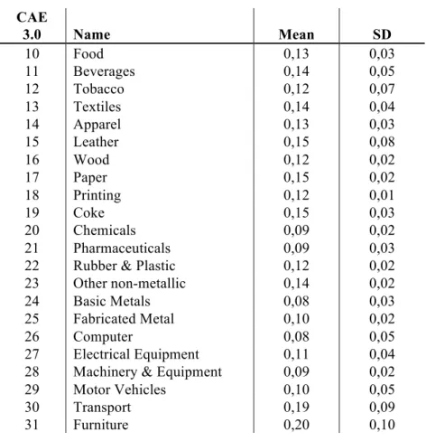
CAE 2.1 to CAE 3.0 as previously described. Summary statistics for leverage of the
different industries are provided in Table 1.
Table 1: Summary Statistics Industry Leverage
CAE
3.0 Name Mean SD
10 Food 0,13 0,03
11 Beverages 0,14 0,05
12 Tobacco 0,12 0,07
13 Textiles 0,14 0,04
14 Apparel 0,13 0,03
15 Leather 0,15 0,08
16 Wood 0,12 0,02
17 Paper 0,15 0,02
18 Printing 0,12 0,01
19 Coke 0,15 0,03
20 Chemicals 0,09 0,02
21 Pharmaceuticals 0,09 0,03
22 Rubber & Plastic 0,12 0,02
23 Other non-metallic 0,14 0,02
24 Basic Metals 0,08 0,03
25 Fabricated Metal 0,10 0,02
26 Computer 0,08 0,05
27 Electrical Equipment 0,11 0,04
28 Machinery & Equipment 0,09 0,02
29 Motor Vehicles 0,10 0,05
30 Transport 0,19 0,09
31 Furniture 0,20 0,10
Graph 1: Markup over time: Markup countercyclicality in transport industry
In Graph 1 the red line represents markup growth of the transport industry. The blue
line represents real GDP growth. This example clearly illustrates the counter cyclicality
-0,3 -0,2 -0,1 0 0,1 0,2 0,3
04 05 06 07 08 09 10 11 12 13
Real GDP Growth
of markups. When the economy grows markup falls and during economic downturn
markup increases4.
2.2 Results from the industry level analysis and interpretation
Following the two hypotheses the analysis involved two regressions. First, a standard
Ordinary Least Squares regression of markup against the proxy of negative economic
activity -log(GDP) was performed. Second, markup is regressed against negative
economic activity, lagged leverage, and an interaction term between lagged leverage
and negative economic activity to test if there is a joint effect of leverage and economic
activity on markups over the given period.
In the first regression of markup against the proxy of negative economic activity
demand shocks -log(GDP), a negative correlation of economic activity and industry
markups is found. The results in Table 2 show that for a 1,00% decline in real GDP
there is a 5.33% increase in markups. Further, the negative coefficient of economic
activity is significant at the 1.00% significance level as it has a p-value of 0.00%. This
rejects the null hypothesis of no effect. The R-squared statistic assesses the strength of
the relationship between the model and the response variable. 13.27% of variation in the
dependent variable is explained by the model. This is acceptable taking into account
that other factors are likely to have significant effect on markups. Some of those factors
are explored in the next regression. The OLS regression uses
heteroscedasticity-consistent standard error estimates to correct against a potential violation of the OLS
independent variable. The results provide support for counter cyclicality5. Note,
however, that the effect of economic downturns increases markups more than economic
growth decreases markups. To find support for the theory by Chevalier and Scharfstein
(1996) that firms increase prices during economic downturn, the regression is run using
log of prices instead of markups. The regression shows a significant positive impact of
economic downturn on prices6. The result from the Portuguese manufacturing industry
provides evidence for countercyclical behaviour of markups. This means that in the
given time between 2004 and 2013, on average, firms of the Portuguese manufacturing
sector increased markups in response to economic downturns. Hence, these results are
in line with Chevaliers and Scharfsteins (1996) theory of markup counter cyclicality and
Bolton and Scharfstein’s (1990) predatory pricing theory. This is also consistent with
Campello’s (2001) work for the United States.
The results for the second regression of markups against negative economic activity,
lagged leverage, and an interaction term between lagged leverage and negative
economic activity are shown in table 3. Here an ordinary least squares fixed-effect
regression7 is applied. The fixed effect regression looks only at within industry
variation. It allows controlling for unobserved heterogeneity as long as it is fixed over
time. Further, the interaction term allows testing for a combined effect of leverage and
negative economic activity. The coefficient of the interaction term is positive and large.
5 The output for the regregssion of economic growth on markups can be found in appendix 3.
Table 2
OLS Regression Markups on the Negative Economic Activity (N = 198)
Table 2 shows the OLS regression of markups on the negative log of economic activity
between 2004 and 2013 on the basis of yearly data.
Markups Coef. Robust SE
Negative Economic Activity 5.3328** 0.8797
Constant 0.0219 0.0173
R2 0.1327
36.74**
0.2589 F
Root MSE
*p < .05. **p < .01.
This suggests a remarkable joint effect of leverage and negative activity. More
precisely, it means that higher debt during recession led markups to increase more
significantly. This finding is significant at the 5% significance level. Consequently, the
null hypothesis of no joint effect is rejected. Again, this is in line with Chevalier and
Scharfstein’ finding (1996) and Campello’s finding (2001).
The result suggests that highly leveraged firms are the ones that tend to increase markup
when GDP goes down. The industry analysis has provided evidence for both – markup
counter cyclicality and a joint effect of leverage and economic downturn on markups.
2.3 Limitations
have an impact on markups and move together with economic activity. An obvious
example are costs that affect the entire industry such as energy prices.
To find direct support for the idea that firms with relatively more debt increase their
prices in response to demand shocks the same regression is run with prices instead of
markups and leads to comparable significant results. The underlying idea is that
companies may very well decrease markups due to an increase of costs.
Table 3
FE-OLS: Markups on economic activity, lagged leverage, and interaction term (N=198)
Table 3 shows the Fixed Effects OLS regression of markups on the negative log of
economic activity, leverage, and an interaction term of leverage and negative economic
activity for the time period between 2004 and 2013 on the basis of yearly data.
Markups Coef. Robust SE
Negative Economic Activity 1.3147 2.2103
Leverage
Leverage*Negative Economic Activity
0.6474
30.7425*
0.7501
R2 0.2434
3.91**
0.2574 F
Root MSE
*p < .05. **p < .01.
3. Firm Level Analysis
Whereas the industry-level analysis dealt with markups, this section focuses on the
effect of leverage on competitive performance contingent on capital structure. The
growth. The theoretical link with the findings from the industry analysis is that firms
compete primarily on the basis of prices and that, by setting lower prices, they can
accelerate sales growth to attain a higher market share. Following Campello (2001), this
section identifies exogenous shocks to the competitive environment. For the Portuguese
economic environment, the 2008 financial crisis has been considered the worst crisis
since the Great Depression (Reuters, 2009). It affected firms’ financial structure in a
way that could not be anticipated by investors or managers. The 2008 crisis’ systemic
nature makes it an ideal setting for testing. The effect of the crisis was not only felt in
certain firms or industries but affected almost all industries at the same time. Still,
according to the theoretical model of Chevalier and Scharfstein (1996), firms should
react differently contingent on their capital structure. Therefore, the objective of this
section is to analyse and compare sales-debt sensitivity between high leveraged and low
leveraged firms.
3.1 Data
The analysis is performed on firm level data. The existence of financial data for a large
set of small and medium Portuguese companies differentiates this analysis from
previous work. Whereas previous work relied on either industry averages or samples
this analysis is based on a census of Portuguese companies. The census of firm-level
financial data was obtained via the ‘IES - Informação Empresarial Simplificada’8
(Instituto Nacional de Estatistica, 2015). Data on sales, fixed assets, total assets, and
leverage were collected for all Portuguese firms for the time range from 2004 to 2010.
excluded from the final testing during the process of data cleansing. Data cleansing
involved the removal of small companies and individuals that were subject to simplified
accounting and, as a consequence, did not report leverage or assets. Examples for these
companies were small cafes, auto repairs, and individuals such as lawyers. Further, for
many companies no more data existed after 2007. A possible explanation for this is that
many companies went out of business following the 2007 financial crisis. Thus, the
remainder is the universe of registered companies in Portugal with organised accounting
that provided a data horizon large enough for testing. The final test was performed on
the basis of 410,336 observations using yearly data.
3.2 Analysis
Campello’s methodology (2001) involves a two-step regression. This helps to reduce
the probability of a type I error. That is the probability of inferring that capital structure
has a significant effect when in fact it does not. The literature review demonstrated links
between capital structure and competitive performance. However, a series of other
factors can influence the competitive performance of a firm. Therefore, the empirical
model includes three other variables next to leverage. First, past performance measured
as one lag of sales growth was taken into account. Second, investments in property,
plant, and equipment (PPE) were considered. The underlying intuition is that good
investments in PPE improve a firm’s competitive performance. In manufacturing, for
instance, obtaining automation machinery or a larger production site to increase
capacity is likely to be followed by an increase in sales assuming the existence of
demand. Third, investments into strategic assets or in Research and Development can
regressed against its past value and the past change in PPE, the past value of total assets,
and past leverage as shown in Equation 4.
Equation 4: First-step regression
Δlog (!"#$%)!
,! =!+αΔlog (!"#$%)!,!!!+βΔlog (!!")!,!!!+γlog (!""#$")!,!!!
+!"#$#%&'#!
,!!!+!!,!
To measure competitive performance a firm’s industry-adjusted sales growth is used.
The advantage of this measure is that it can be compared across industries. The
drawback is that competitive performance is not only measured by market share. It also
depends largely on how well a company is able to put its strategy into practice, and how
the stock market evaluates that reflected in the share price (Kaplan & Norton, 2001).
However, relative market share was preferred due to its comparability and
representativeness of product market competition. Equation 5 shows the calculation of a
company’s industry-adjusted sales growth. The difference between company sales
growth and industry sales growth is divided by the absolute value of industry sales
growth. The absolute value is used to overcome the fallacy of negative and positive
growth numbers. Looking at Equation 4 imagine company sales growth being positive
and industry sales growth negative. Without using the absolute value of industry sales
growth in the denominator, the resulting number for company industry-adjusted sales
Equation 5: Industry-adjusted sales growth
!"#$%&'"!"!"#$%&'(!"#$!!"#$%ℎ!
,! =
!"#$%&'!"#$!!"#$%ℎ!,!−!"#$%&'(!"#$!!"#$%ℎ!,!
!"#$!"#$!"#$!!"#$%ℎ!,!
!"#$%!"#$%ℎ !,!=
!"#$!!,!−!"#$!!,! −1 !"#$!!,!
−1
To obtain the PPE and the total assets variables relative to the industry average, PPE
and total assets were adjusted according to the same principle as industry-adjusted sales
growth. This way a company is not defined by its own measure but relative to its
competitors. This is important when later dividing into high debt and low debt groups.
Leverage is measured as the long-term debt-to-asset ratio and also relativised against
industry leverage. Unlike the other variables industry leverage is calculated by using the
asset-weighted long-term debt-to-asset ratio as can be seen in Equation 6. This measure
is better than a simple average due to its asset-weight. This weight lets the financing
patterns of significant companies influence the industry average more than the financing
of smaller negligible companies. Hence, a representative picture is obtained.
Equation 6: Leverage
Leverage!"=
!""#$"!" !""#$"!" ! !!! ! !!! ∙ !"#$!"
!""#$"!" =
!"#$!" !""#$"!" ! !!! ! !!!
(weight based on assets x debt-to-asset ratio)
First, the regression from the empirical model in Equation 4 is run over the entire data
set to test the fit of the model. The results are displayed in Table 4.
investment in assets leads to a significant increase in sales. Most importantly, leverage
significantly impacted sales growth. Contrary to initial expectations the results show
that last year’s change in sales growth has no impact on current year’s sales growth. All
stated results are significant at the 1% significance level.
Table 4
OLS: Sales growth on itself, PPE, assets, and leverage (N=410,336)
Table 4 shows the OLS regression of sales growth on its past value and the past change
in PPE, the past log of total assets, and past leverage between 2004 and 2010 on the
basis of yearly data. All explanatory variables are lagged one period to reflect previous
period’s effect of decisions on competitive performance.
Sales Growth Coef. Robust SE
Sales Growtht-1 0.0000117 0.0000144
PPE Growtht-1
Assetst-1
Leveraget-1
0.0044285**
7.3000658**
2.50e-06**
0.0006788
1.210572
4.68e-07
R2 0.0002
21.52**
70.162 F
Root MSE
*p < .05. **p < .01.
However, the R-squared of 0.02% and a large MSE do not suggest a good fit. Note that
assumption that investments could take more time to materialise9. However, there are
no significant relationships for any lag larger than one.
In the second step, for each regression run the leverage coefficient, δ, is extracted and
set up as time series. The leverage coefficient series is then run against four lags of
economic activity and a time trend. The proxy for economic activity is -log(GDP) as
used in the industry level analysis. The regression model can be seen in Equation 7.
Equation 7: Second-step regression
δ! =!+ ϕ!ΔActivity!!! !
!!!
+γ!"#!"!+!!
3.3 Results from the firm level analysis and interpretation
Campello’s theory (2001) posits that firms that are highly leveraged relative to their
industry rivals will have higher sales debt sensitivity than firms that are less leveraged
relative to their industry peers during economic downturn. To compare high and low
debt firms two groups are created representing the bottom 25 per cent and the top 25 per
cent in a ranking based on industry-adjusted leverage. The effect is that industries are
ranked according to the degree of competitor’s leverage level for each year t.
Thereafter, the bottom 25 per cent and the top 25 per cent are extracted resulting in two
groups – low debt industries and high debt industries. The resulting data set is 100,037
observations per group. The high debt and low debt datasets are used to perform the
first-step regression from Equation 5. Thereafter, for each year the delta coefficient is
extracted and saved as time series. The resulting time series is then regressed against
one lag of economic activity as described in the second-step regression in Equation 7.
The outputs for these regressions are reported in appendix 3. Unfortunately, no
inference can be drawn from these regressions. This is mainly due the limited number of
observations that stem from the small time range and frequency of the data.
Remarkably, the coefficient for high debt companies is a lot larger (-6.12) than the one
for the low debt companies (-2.99). This would imply that that the more leveraged firms
experience more sales debt sensitivity and would be in line with the expectation and
Campello’s (2001) findings that relatively highly leveraged firms suffer more market
share loss than their relatively low leveraged rivals. Although the coefficients point into
the expected direction they are not significant. In addition to that, the number of
observations that this result is based on is not sufficient. Consequently, no direct
support for the presented theory is obtained from the firm-level analysis.10
3.4 Limitations
The primary limitation in the firm level analysis is the lack of longitude and frequency.
Whereas the dataset covered a census of all Portuguese companies the given time range
of the firm level data only goes from 2004 to 2010. Using yearly frequencies this results
in only seven periods. In the first step regression in Table 4 all but one coefficient are
significant. However, when moving to the second step regression observations are
reduced to the number of periods t namely 7. When running the second regression two
observations are lost due to the lag and the change. Five observations, although they
represent coefficients derived from a much larger dataset, cannot capture the sales debt
sensitivity with respect to economic downturns. To counteract this deficit there are two
solutions. Either a dataset with larger longitude is used or a higher frequency such as
quarterly or monthly data obtained. In his paper Campello (2001), for example, used
quarterly data from 1976 to 1996. With this frequency and longitude of Campello’s data
that allowed for more precise and time sensitive results.
4. Conclusions
This paper investigated the effect of capital structure on competitive behaviour on two
levels. First, the effect of leverage on markups during demand shocks was analysed on
the industry level. The result of the analysis provided evidence for Chevalier and
Scharfstein’s theory of counter cyclicality of markups (1996). A 1% decline in real
GDP was followed by a 5.3% increase in markups. However, the markup-increase for
GDP decline was stronger than the markup-decrease for GDP growth. Another
important result from the industry analysis provided support for Bolton and
Scharfstein’s original theory (1990). Their theory suggested that during economic
downturns more debt-constrained firms are unable to keep up with price competition
and, consequently, increase markups. Accordingly, a positive joint effect of debt and
economic downturns on markups is observed. Both results – markup counter cyclicality
as well as the joint effect of leverage and debt on markups – are in line with Campello’s
findings (2001).
Second, the effect of capital structure on competitive performance was examined at the
industries in which competitors are highly leveraged experience higher sales debt
sensitivities. The general model provides a bad fit. Nevertheless, there is a significant
effect of leverage on competitive performance. However, the final test on subgroups
representing relatively high leveraged and relatively low leveraged companies as
compared to their industries does not yield significant results. Consequently, no
significant results about the effect of capital structure on competitive performance could
be established. In conclusion this paper provides evidence for markup counter
cyclicality and a joint effect of debt and negative economic activity, at industry level.
Overall the evidence from the Portuguese companies provides support for former
theories on the industry level. For the firm level analysis, however, no significant result
could be obtained. This is due to the fact that the employed model required more
observations in terms of longitude and frequency. For this the author would like to
encourage revisiting the proposed methodology within the Portuguese context at a later
point in time with more accumulated data or with a higher data frequency. Moreover,
results are subject to a series of limitations of which three are worth mentioning. First,
leverage, markups, competitive performance, and resulting product market outcomes
might be influenced by a third unobserved variable. Second, a relatively small time
range and data frequency can have very well biased the accuracy of the results. Third,
although a theoretical model from the US was successfully applied in the Portuguese
context, the Portuguese manufacturing industries and their companies are a very small
portion of the global market. In fact the Portuguese GDP represents only around 0.4%
market has been on a decline and economic powers such as China, India and Indonesia
provide interesting and possibly more relevant grounds for future academic research.
This is why the author encourages further research and testing of the theory supported
References
Bils, M. (1987). The Cyclical Behavior of Marginal Cost and Price. The American Economic Review, 77(5), 838-855.
Bloomberg L.P. (2015) Portugal GDP: real growth rate 01/01/04 to 31/12/04. Retrieved November 19th, 2015 from Bloomberg terminal.
Bolton, P., & Scharfstein, D. (1990). A Theory of Predation Based on Agency Problems in Financial Contracting. The American Economic Review, 80(1), 93-106. Brander, J., & Lewis, T. (1986). Oligopoly and financial structure: The limited liability
effect. American Economic Review, 85, 956-970.
Brooks, C. (2008). Panel Data. In Introductory Econometrics for Finance (Second ed., pp. 487-510). Cambridge: Cambridge University Press.
Campello, M. (2001). Capital structure and product markets interactions: Evidence from business cycles. Journal of Financial Economics, 68, 353-378.
Chevalier, J., & Scharfstein, D. (1996). Capital Market Imperfections and
Countercyclical Markups: Theory and Evidence. The American Economic Review, 86(4), 703-725.
Chirinko, R., & Singha, A. (2000). Testing static tradeoff against pecking order models of capital structure: A critical comment.Journal of Financial Economics,58, 417-425.
Harris, M., & Raviv, A. (1990). Capital Structure and the Informational Role of Debt. The Journal of Finance, 45(2), 321-349.
Harris, M., & Raviv, A. (1991). The Theory of Capital Structure. The Journal of Finance, 46(1), 297-355.
Kaplan, R., & Norton, D. (2001). Transforming the Balanced Scorecard from Performance Measurement to Strategic Management: Part I. Accounting Horizons, 15(1), 87-104.
Economias. (2015, May 6). O que diz a Lei Sobre Horas Extras, Domingos e Feriados - Economias. Retrieved December 26, 2015, from http://www.economias.pt/o-que-diz-a-lei-sobre-horas-extras-domingos-e-feriados/
Instituto Nacional de Estadística (INE). (2003). Classificação Portuguesa das Actividades Económicas Rev.2.1. Instituto Nacional de Estadística (INE). Instituto Nacional de Estadística (INE). (2007). Classificação Portuguesa das
Actividades Económicas Rev.3.0. Instituto Nacional de Estadística (INE). Instituto Nacional de Estatistica. (2015, October 26). IES - Informação Empresarial
Simplificada. Retrieved from http://www.ies.gov.pt/site_IES/site/servicos.htm Jensen, M., & Meckling, W. (1976). Theory of the Firm: Managerial Behavior, Agency
Costs and Ownership Structure. Journal of Financial Economics, 3, 305-360. Klemperer, P. (1995). Competition when Consumers have Switching Costs: An
Overview with Applications to Industrial Organization, Macroeconomics, and International Trade. The Review of Economic Studies, 62, 515-539.
Modigliani, F., & Miller, M. (1958). The Cost of Capital, Corporation Finance and the Theory of Investment. The American Economic Review, 48(3), 261-297.
Reuters. (2009, February 27). Three Top Economists Agree 2009 Worst Financial Crisis Since Great Depression; Risks Increase if Right Steps are Not Taken. Retrieved December 29, 2015, from http://www.reuters.com/article/idUS193520 27-Feb-2009 BW27-Feb-20090227
Rotemberg, J., & Woodford, M. (1991). Markups and the Business Cycle. In NBER Macroeconomics Annual 1991, (Vol. 6, pp. 63-140). MIT Press.
Shyam-Sunder, L., & Myers, S. (1999). Testing Static Trade-off Against Pecking Order Models of Capital Structure.
Trading Economics. (2015, December 31). Portugal GDP | 1960-2016 | Data | Chart | Calendar | Forecast | News. Retrieved January 4, 2016, from
http://www.tradingeconomics.com/portugal/gdp
APPENDIX
Appendix 1: The ‘robust’ option in STATA
This Appendix clarifies the mechanics of the robust option and how it corrects for
potentially violated assumptions in the regression. Using ‘robust’ standard errors solves
many problems relating to unfulfilled assumptions (Verardi and Croux, 2009). A
side-effect of using the option is a more conservative approach to testing.
SATA’s ‘robust’ option was used for each regression in this paper and has the following
mechanics. It weighs the observations differently based on how well behaved these
observations are, making the OLS a weighted least square regression. The robust option
obtains the Cook’s distance estimate. The Cook’s distance estimate measures the effect
of deleting a given observation. Data points with large residuals may distort the
outcome and accuracy of a regression. It holds that the larger the estimate, the more
distorting the data point. The robust regression drops any observation with Cook’s
distance greater than 1. Thereafter an iteration process begins in which weights are
calculated on the basis of residuals. Two types of weights are used. First, Huber
weighting that gives observations with small residuals a weight of 1 and observations
with larger residuals smaller weight. Second, via biweighting all cases with a non-zero
residual get a slightly reduced weight. This results in the most influential point being
dropped and the cases with large absolute residuals are down-weighted (Verardi and
Appendix 2: Fixed Effects Regression in STATA
Appendix 2 aims to clarify the specificities and motivation behind using a fixed effects
model in the industry analysis of the paper. The analysis is based on panel data – data
comprising information across time and space. The standard pooled regression assumes
that the average values of the variables and the relationships between them are constant
over time and across all the cross-sectional units in the sample. Consequently, it does
not fit panel data, as average values will very likely differ across entities (Brooks,
2008). The fixed effects regression is different in that is assumes fixed effects. It
imposes time independent effects for each entity that are possibly related with the
regressor. It accounts for effects on the time level t and in the entity level i. A standard
fixed effects model is shown in Equation A2.1.
Equation A2.1 Fixed Effects model
yit =α+βxit +µi +vit
The disturbance term is divided into an individual specific effect µi and the remainder
disturbance vit that varies over time and entities. The individual effect µi includes the
variables that affect the dependent variable cross-sectionally but not over time. In the
dataset of the analysis this can be the industry a firm operates in. The remainder
disturbance captures the effect of variables that vary over time and entity. The fixed
effects model is appropriate for the panel data used because the objective is to measure
fixed effects such as industry and time variant effects such as markups. The
Durbin-Wu-Hausman test is often used to discriminate between the fixed and the random
Appendix 3: Complementary estimates and regression results
A3.1 Campello (2001) Replication: OLS Markups on -Δlog(GDP) US data (N = 700)
This table reports the OLS regression of markups on the negative log of economic
activity for the time period between 1984 and 1996 on the basis of monthly data.
Markups Coef. Robust SE
Negative Economic Activity 6.935739** 2.140439
Constant 0.0897611* 0.0326066
R2 0.0142
10.50**
0.28318 F
Root MSE
*p < .05. **p < .01.
A3.2 Campello (2001) Replication: FE-OLS: Markups on -Δlog(GDP)), Leverage, and
Leverage* -log(GDP) on the basis of US data (N=700)
This table reports the Fixed Effects OLS Regression of markups on a proxy of negative
economic activity, leverage and the interaction term of leverage and negative economic
activity for the time period between 1984 and 1996 on the basis of monthly data.
Markups Coef. Robust SE
Negative Economic Activity -3.281413 7.97016
Leverage
Leverage*Negative Economic Activity
1.67318*
43.61785
0.59271
28.75445
R2 0.1541
A3.1 and A3.2 are the replication of Campello’s (2001) work on the replication of the
set he used. The data included sub industries of the American manufacturing industry in
the time range between 1984 and 1996. The replication was done as an exercise to
understand data and methodology of his paper as well as to analyse if it could be
applied to Portuguese data and context. The results of the replication were similar to his
original work. In the replication of the American data a major difference was the
leverage series that he had obtained using a sample of company information unavailable
to the public.
When comparing the findings on the American data with the findings from the
Portuguese context similarities are found. A3.1 displays the positive effect of economic
downturn on markups as found in the context of the Portuguese data. A3.2 shows a
positive relationship between the interaction term of leverage and economic downturn.
Although the latter coefficient is not very significant it is in line with the result from the
Portuguese data.
A3.3 Industry Analysis: Regressing negative economic activity against price (N = 198)
This table reports the OLS regression of the negative log of economic activity on the
logarithm of prices (instead of markups) between 2004 and 2013 using yearly data.
Price Coef. Robust SE
Negative Economic Activity 1.009294 ** 0.3318921
Constant 0.0061897** 0.0061897
R2 0.0513
9.25**
0.0945 F
Root MSE
The regression in A3.3 shows that during economic downturns prices increase
significantly. For a 1% decrease in GDP prices increase by approximately 1%. The
result is significant at the 1% level This is in line with the Chevalier and Scharfstein’s
(1996) theory that firms are unable to cut prices during recessions. The R-squared of the
model with price is lower (5.13% < 13.27%) than of the model with markups. This
means that GDP explains more variation of markups than for prices.
A3.4 Industry Analysis: OLS Markups on positive economic activity (N = 198)
This table reports the OLS regression of markups on the positive log of economic
activity between 2004 and 2013 on the basis of yearly data.
Price Coef. Robust SE
Positive Economic Activity -3.577047 ** 0.9263732
Constant 0.0260996** 0.0173899
R2 0.0785
14.91**
0.26689 F
Root MSE
*p < .05. **p < .01.
Complementary to testing whether companies increase markups during crisis this
regression tests whether companies decrease markups during booms. The result shows
that for a 1% increase in GDP markups decrease by 3.58%. The result is significant at
the 1% significance level. This is in line with Chevalier and Scharfstein’s (1996) theory
of counter cyclicality. However, it is noteworthy that markups increase stronger during
A3.5 Second step Regressions Firm Level Low Debt Group (N=4)
This table reports the OLS regression of the time series vector extracted from the first
step regression on past negative economic activity between 2004 and 2010 on the basis
of yearly data. The subsample is derived on the basis of the extracted delta coefficient
from the first regression for each year t and reflects the bottom 25% of companies in
terms of debt.
Markups Coef. Robust SE
Negative Economic Activity -2.988037 1.136014
Constant
Trend
-0.4729765
0.1839865
0.061911
0.015428
R2 0.0142
10.50**
0.28318 F
Root MSE
A3.6 Second step Regressions Firm Level High Debt Group (N=4)
This table reports the OLS regression of the time series vector extracted from the first
step regression on past negative economic activity between 2004 and 2010 on the basis
of yearly data. The subsample is derived on the basis of the extracted delta coefficient
from the first regression for each year t and reflects the top 25% of companies in terms
of debt..
Markups Coef. Robust SE
Negative Economic Activity -6.122926 10.96523
Constant
Trend
-0.2810392
0.0614733
0.061911
0.5976229
R2 0.2421
0.28
0.1986 F
Root MSE
*p < .05. **p < .01.
These regression outputs represent the final result of the firm level analysis. Despite
their insignificance their coefficient point into the right direction. If this was significant
– during crisis companies that are high leveraged relative to their industry peers, would
have more negative impact on their sales than companies that are low leveraged relative
Appendix 4: Data for firm level analysis
The dataset is obtained using two sources. The first source is a census of companies
(IES), which includes all resident firms, excluding the financial sector and holding
companies. The IES covers around 1 million companies per year for the period
2004-2010. Around seven hundred thousand are private individuals, which have a simplified
reporting and are excluded from the analysis. These are small businesses without
obligations of maintaining an organised accounting. Some examples are hairdress
saloons, restaurants, cafes, carpenters, construction services and related, auto repair,
auto sales, wholesale, diverse retail, lawyers, accountants, consultants, architects,
educational services, medical services, etc. The remainder is the universe of registered
companies in Portugal with organised accounting of over three hundred thousand per
year. The IES contains financial information (balance sheet, P&L, investment) and