Biomechanical Simulation of the Load Distribution in Dental Implants

Faculdade de Engenharia da Universidade do Porto

Biomechanical Simulation of the Load Distribution

in Dental Implants

João Paulo Dias Andrade

Dissertation elaborated on

Integrated Master in Bioengineering

Branch of Biomedical Engineering

Coordinators: Prof. Aníbal Matos

Prof. Germano Veiga

Prof. Francisco Caramelo

iii

Biomechanical Simulation of the Load Distribution

in Dental Implants

Dissertation approved by the jury:

 President: Renato Natal Jorge

 Examiner: Nuno Chichorro Ferreira

 Coordinators: Aníbal Matos, Germano Veiga, Francisco Caramelo

_______________________________ (Coordinator)

v

Abstract

Thanks to the collaboration of interdisciplinary teams, the success rate of correctly designed, manufactured and placed dental implants has been increased up to 95% worldwide [1]. These numbers can still be improved by the aid of experimental models, such as photoelastic or virtual, which play an important role in this field. Using these models, it is possible to study the stress and strain distributions on mandibles, implants or prosthesis.

The objective of the dissertation is to understand the correlation between the strain results on the mandible when a load is applied on a dental prosthesis and implants in both models tested: experimental three-dimensional photoelastic and virtual Finite Elements.

For this matter, virtual three-dimensional models with the same shape and dimensions of a photoelastic mandible, titanium dental implants and milling alloy on Cobalt basis prosthesis were designed. Using Finite Element Analysis (FEA), numerical simulations were carried out equally to the experimental ones, done prior to this work.

The strain results were compared and a significant agreement was found between both methods with a total error percentage of 8.3% ± 9.6 and a Pearson’s correlation coefficient of 0.836 (p < 0.01)

This suggests that both models are strong and significantly correlated and a cross-validation of both techniques was found for three-dimensional non-destructive assays on a mandible assembled with dental prosthesis and implants.

vii

Resumo

Devido à colaboração de equipas interdisciplinares, a taxa de sucesso da colocação de implantes dentários corretamente modelados, fabricados e colocados tem crescido até 95% em todo o mundo [1]. Estes números podem ainda ser melhorados com a ajuda de modelos experimentais, sejam fotoelásticos ou virtuais, que desempenham um papel importante neste ramo. Usando estes modelos, é possível estudar as distribuições de tensão e deformação em mandíbulas, implantes ou próteses.

O objetivo da dissertação é entender a correlação entre os resultados da deformação na mandíbula quando uma carga é aplicada na prótese dentária e implantes nos dois modelos testados: fotoelástico experimental tri-dimensional e virtual de Elementos Finitos.

Neste sentido, foram desenhados modelos virtuais tri-dimensionais com a mesma forma e dimensões que a mandíbula fotoelástica, implantes dentários de titânio e prótese numa liga de cobalto.

Usando a Análise de Elementos Finitos, foram realizadas simulações numéricas da mesma forma que os testes experimentais, feitos anteriormente a este trabalho.

Os resultados da deformação foram comparados e foi encontrada uma concordância significativa entre os dois métodos com uma percentagem de erro total de 8,3% ± 9,6 e um coeficiente de correlação de Pearson de 0.836 (p < 0.01).

Estes resultados indicam que ambos os modelos são forte e significativamente correlacionados e que se encontrou uma validação mútua das duas técnicas para ensaios tri-dimensionais não-destrutivos em mandíbulas contendo implantes dentários e próteses.

ix

Acknowledgments

Este documento, mais que o resumo de um trabalho de meses, é símbolo de 5 anos de trabalho e empenho que, aliados a todos os risos e choros se tornaram inesquecíveis.

Em primeiro lugar, o meu muito obrigado a todos os que tornaram este trabalho possível: ao Professor Germano Veiga, por toda a disponibilidade demonstrada, ajuda e orientação durante todos estes meses em todas as fases do trabalho, sem exceção. Ao Professor Francisco Caramelo, também pela constante disponibilidade e ajuda preciosa no decorrer do trabalho, nomeadamente na segmentação, nas constantes dúvidas esclarecidas e na revisão deste documento. Ao Doutor Pedro Brito, pela TAC da mandíbula usada, esclarecimento dos vários conceitos relacionados com o tema e com os próprios métodos do trabalho, bem como com o seu enquadramento na investigação decorrente.

Kipp… Kiitos a todos os que, independentemente da nacionalidade ou cultura, me ajudaram a construir um lar nos meses de Erasmus, oferecendo-me uma experiência única.

À fantástica família Metal&Bio, com quem aprendi quem quero ser. Que me fez ser parte de um rio negro de capas ondulantes marcadas a preceito por Momentos e Irmãos. A todos vós, acima ou abaixo, não agradeço.

Um especial obrigado a 08/09 (e a quem por este grupo passou) por terem estado sempre do meu lado, nunca me faltando com nada, fossem ajudas nos trabalhos de grupo, explicações sobre as várias matérias, uma palavra, um ombro, um sorriso ou uma garrafa.

A ti, Helena, por teres sido a minha cúmplice nestes anos imortais, que vivia todos novamente. Por me teres aturado nas horas boas em que sou irritante e nas horas más em que sou ainda mais. Muito, muito obrigado.

Aos meus avós que nunca me deixam só e sempre me relembram do menino que há em mim, aos meus tios e as suas palavras amigas, ao companheirismo e amizade dos meus primos e às vidas que foram aparecendo e crescendo sem se dar por isso nestes anos.

Finalmente ao meu irmão por ter sempre uma goleada no FIFA pronta quando apareço ao fim de semana e, principalmente, aos meus PAIS, pelos sacrifícios feitos para que eu seja a pessoa mais sortuda deste mundo. As minhas desculpas pelo meu feitio muitas vezes difícil de aturar e um enorme obrigado, pela amizade, ensinamentos e raspanetes (vamos tentar que sejam menos).

E a ti, “Porto das pontes, cidade”, cujos “becos cinzentos pintados de outras saudades”, levam agora também a minha pincelada.

xi

“It ain't what you don't know that gets you into trouble. It's what you know for sure that just ain't so.” nobody knows for sure the author

xiii

Table of Contents

Abstract ... v

Resumo ... vii

Acknowledgments ... ix

List of figures ... xv

List of Tables ... xvii

Acronyms and Symbols... xviii

Chapter 1 ... 1

Introduction ... 1

Chapter 2 ... 3

Dental Implants ... 3

2.1 - History of Dental Implants ... 3

2.2 - Dental Implant Insertion Procedures ... 4

2.3 - Types of Implants ... 5

2.4 - Bridges ... 5

Chapter 3 ... 7

Dental Biomechanics ... 7

3.1 - Materials of Dental Implants ... 8

3.2 - Cortical Bone Properties ... 9

3.3 - Trabecular Bone Properties ... 12

3.4 - Periodontal Ligament ... 13

Chapter 4 ... 15

4.2 - Finite Elements Method ... 20

Chapter 5 ... 23

5.1 - Photoelasticity ... 23

5.2 - Finite Elements Method ... 24

Chapter 6 ... 29

Results and Discussion ... 29

6.1 - Photoelasticity ... 29

6.2 - FEM and Methods’ Comparison ... 31

Chapter 7 ... 37

Conclusion... 37

xv

List of figures

Fig. 2.1. Dental implant with abutment and custom-made crown comparison with a

normal tooth [9] ... 3

Fig. 2.2. Dental implants after the one-stage implantation (a) and after the first phase of a two-stage implantation (b) [15] ... 4

Fig. 2.3. Different types of dental implants [10] ... 5

Fig. 2.4. Representation of a bridge supported by two dental implants [19]. ... 6

Fig. 3.1. Bone representation [25] ... 7

Fig. 3.2. Active and passive creep as a function of the stress level normalized to ultimate stress: 33/ 33u: 0.2 (1); 0.3 (2); 0.4 (3); 0.5 (4); 0.6 (5); 0.7 (6) [10]... 11

Fig. 3.3. Stress-strain curve at 2.5 per cent (a) and 10.5 per cent (b) moisture level for 10 -5_{/s strain rate [10] ... 11}

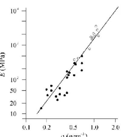
Fig. 3.4. Correlation of density and elastic modulus in tension (filled circles) and compression (empty circles) for trabecular bone [10] ... 12

Fig. 4.1. Plane polariscope and birefringent effect. Adapted from [43]... 16

Fig. 4.2. Representation of reflection polariscope and its relation with the photoelastic object and reflective adhesive. Adapted from [43] ... 17

Fig. 4.3. Representation of the resulting element from the photoelastic analysis in three orthogonal directions [38] ... 18

Fig. 4.4. Sketch showing stress components on a three-dimensional element. ... 19

Fig. 4.5. Finite Elements mesh representation for a given part. Adapted from [46] ... 20

Fig. 5.1. Robot performing mastication simulation under polarized light ... 23

Fig. 5.2. Three-dimensional CAD model of the prosthesis used in the experimental tests, which served as a mold for the virtual model used in the FEM test. Teeth are numbered according to the FDI (World Dental Federation) two-digit notation [54]. ... 24

Fig. 5.4. 3D assembled and meshed objects used in the simulations. Dark yellow: mandible; blue: prosthesis; red: dental implants in a) and b). Close up transparent view in c) and fixation boundary condition area represented delimited by the red line in d). Black arrow in a) points at tooth 46, where the pressure is applied. ... 26 Fig. 5.5. Top view of an horizontal cut of the meshed mandible showing the endpoint of

three of the four implants (black circumferences) and nine black dots tangent to one of them along the light path representing the analysed elements. ... 26 Fig. 6.1. Photoelasticity test photograph showing the photoelastic mandible assembled

with dental implants and prosthesis. It is also visible the piece of the robot that is applying a 200N load on tooth number 46 and the reflective layer posterior to the mandible. Analysed points are coloured and identified in Table 6.1. ... 29 Fig. 6.2. Secondary principal strain difference results for each point represented by their

number and assigned ... 30 Fig. 6.3. General view of the Finite Element’s result for the Maximum Principal Strain of

the model with scale normalized to 0.25 ... 31 Fig. 6.4. Finite Element’s result for the Maximum Principal Strain of the model with scale

normalized to 0.25. Both images show the implant placed on the anatomical right-hand side (closer to the load). a) represents a front view relatively to figure 6.3 and b) shows the view from the anatomical left-hand side of the same implant. ... 31 Fig. 6.5. Finite Element’s result for the Maximum Principal Strain of the model with scale

normalized to 0.25. Results without the use of the tie constraint. Both images show the implant placed on the anatomical right-hand side (closer to the load). a) represents a front view relatively to figure 6.3 and b) shows the view from the anatomical left-hand side of the same implant. ... 32 Fig. 6.6. Relative retardation values for every point analysed in both FEM and

Experimental methods ... 32 Fig. 6.7. Error Ratio using the real difference between methods’ values. Close to implant

are considered 1-10 and away the rest. On traction are considered 1-5 and 11-21 and on compression the rest. ... 33 Fig. 6.8. Error Ratio using the absolute difference between methods’ values. Close to

implant are considered 1-10 and away the rest. On traction are considered 1-5 and 11-21 and on compression the rest. ... 33 Fig. 6.9. Comparison between the error ratio of the points close under compression and

away under tension. ... 34 Fig. 6.10. Parallel beam of light being refracted when passing through an irregular object

xvii

List of Tables

Table 3.1. Conventional alloys used for medical devices [10] ... 8

Table 3.2. Mechanical properties of CP-Ti types [10] ... 9

Table 3.3. Young’s Modulus (E) and Poisson’s ratio (ν) given by the literature [1, 27] for titanium dental implants ... 9

Table 3.4. Average elastic constants for mandibular corpus in different zones [10] ... 10

Table 3.5. Mechanical properties of cortical and trabecular bone given by some authors. Adapted from [1] ... 10

Table 3.6. Yield and ultimate stress values for axial and torsional loading in cortical bone specimens taken from human femur [28]... 11

Table 3.7. Elastic modulus of individual trabeculae of trabecular bone. Comprarison of different experimental data [10] ... 13

Table 3.8. PDL elastic constants used in different works with FEA [34-36] ... 14

Table 5.1. Mechanical properties of the materials used in the FEM simulations. ... 25

Table 5.2. Mesh properties of the different objects ... 25

Table 6.1. Number identification for the coloured dots in figure 6.1. Numbers are assigned from de bottom to the top for each colour. ... 30

Acronyms and Symbols

List of Acronyms

CP-Ti Commercially Pure Titanium CAD Computer Aided Design

CT Computed Tomography

DeVIDE Delft Visualisation and Image processing Development Environment FDI World Dental Federation

FEA Finite Element Analysis FEM Finite Element Method

NURBS Nun-Uniform Rational B-Splines PDL Periodontal Ligament

List of Symbols

N Cycles of Relative Retardation

ρ Density

f Fringe Constant

δ Light Wave Retardation Distance

M Light Wave Velocity

ν Poisson’s Ratio

G Shear Modulus

ε Strain

K Strain Optical Coefficient

σ Stress

t Thickness

τ Torsional Stress

λ Wavelength

Chapter 1

Introduction

Dentistry plays a key role in people’s life, relatively either to health and welfare. When one or more teeth are missing, its substitution is crucial in order to improve appearance, comfort, speech and self-esteem [1]. Relatively to other prosthetic techniques, dental implants improve these factors, since, once well fixed, they just need the normal oral hygiene as maintenance. The individual also does not live with the inconvenience and embarrassment caused by removable partial or full dentures. Dental implants also ensure sustainability to adjacent teeth and prevent the face to get the old appearance characteristic from missing teeth due to jaw’s degradation [1, 2].

Worldwide statistics show over 95% of success rate of dental prosthesis when the implants are designed, manufactures and placed correctly. Moreover, the survival rate at 15 years was determined as 90% [1]. Although the authors of the study [1] consider this low risk as an advantage, it is thought that there is room for improving even further.

Despite the success, the percentage of the population with a single or multiple dental implants is still low (by 2006 [1] only 15% among the Australians). One of the reasons, is the lack of general understanding of stress characteristics associated to the binomial mandible/implant and its biomechanical behaviour [1].

This study is a contribution to the knowledge in the field and aims at helping dentists all over the world to understand more and more about this engineering part of their work.

The success of an implant depends on factors such as its design and placement technique. The major cause of failure is the insufficient biomechanical bounding between the implant and the surrounding bone due to a deficit in osseointegration. The lack of osseointegration may be caused by infections processes or inadequate load protocols. To prevent infections the placement technique is very important but also the shape of the implant surface since better fitting between bone and the implant surface reduce void spaces where bacteria could growth. On the other hand, large load in implants may promote mobility of the implant and holes for bacteria whereas small load may be insufficient to stimuli osteoblast activity and, consequent, ossseointegration. Therefore, it is important to understand the properties of materials and how they are variable for a better study of dental implants. For instance, it is not fully understood how does bone reacts to increased stress in the peri-implant bone. It is thought that either the bone is stronger than expected or it adapts to increased stress [3].

2 Introduction

The strain induced by stress appears to influence a mechanical and hormonal response, which leads to bone remodelling [4, 5]. Therefore, it is important to study different methods that analyse these strain patterns.

As an addition to this bridge between engineering and dentistry, this work intends to analyse a simpler alternative to non-destructive three-dimensional photoelastic approach as the usual ones, for instance Frozen Stress technique, described in [6] [7] and the comparison with finite elements method.

Finite elements method’s results are a target of maximum attention as well, since its cross-validation with photoelasticity is crucial for the development of the work beyond this dissertation.

Thus, this thesis is intended to serve as scientific support for photoelastic studies carried out in the dentistry field. Their future results are proposed to be here validated.

This document is divided in seven chapters, in order to expose and explore the objectives of the dissertation. Since the general context and objectives of the work is presented here, the second and third chapters are dedicated to dental implants and bone biomechanics, respectively. After these introductory oriented chapters, theory on photoelastic and finite elements methods is explained in chapter four for a better understanding of the experimental procedures described in the following fifth chapter.

Finally, the results of the work and discussion are presented in chapter six and conclusions and future work proposals in the seventh and last section.

Chapter 2

Dental Implants

Dental implants are metal or ceramic devices that replace the root of natural teeth. After implant placing, artificial teeth are attached on its head, enabling the normal function [8], as it is represented in figure 2.1.

Fig. 2.1. Dental implant with abutment and custom-made crown comparison with a normal tooth [9]

This type of devices are one of the most used options to replace a missing tooth, since they ensure adjacent teeth sustainability, prevent the face to get the old appearance characteristic from missing teeth due to jaw’s degradation and are reliable substitutes to teeth for their normal functions [2].

Mastication induces a complex configuration of loading, which can be mainly described by vertical and transversal forces. These forces induce stress not only in implant itself but also in the surrounding bone. Many factors affect the load bearing capacity of this system: type of loading, shape and dimension of the implant, implant surface and quantity and quality of the bone tissue which surrounds the implant [10].

2.1 - History of Dental Implants

Humans have been trying to find ways to replace missing teeth for a long time. Egyptians used trimmed and shaped seashells to hammer into the jaw to replace missing teeth. The shells may have worked as dental implants because of its content on calcium carbonate that could have facilitated osseointegration [11]. Much later, by the 30’s of the XX century,

4 Dental Implants

Vitallium, a chrome alloy, was introduced to dentistry due to its demonstrated passivity. In the 50’s, magnets were implanted in patients’ jaws with another magnet (attractive) inside the patients’ denture. Other technique was a vertical transfixation implant, tapped from under the anterior mandible with a variable number of pins (3 to 7) that protrude into the mouth [12].

By the end of this decade, many clinicians were working with metal so-called blade design implants that were said to integrate with the jaw through the formation of a pseudo-periodontal ligament, which was in fact a connective tissue capsule. Also by this period, Dr. Peringvar Brånemark of Gothenburg, Sweden, and his team reported that bone-anchored titanium bonds irreversibly to the living bone after some time under carefully controlled conditions, without long-term soft tissue inflammation, fibrous encapsulation or implant failure. This phenomenon was named osseointegration by Brånemark himself [11].

Indeed, the first practical application of osseointegration was the implantation of titanium roots in an edentulous patient in 1965, who, by the time of his death, over 40 years later, was using the original dental implants. This is considered the birth of modern implantology. The Brånemark implant (first called Biotes) remain one of the main implant systems available today, and its good acceptance, rapidly led to the oblivion of the blade implants.

2.2 - Dental Implant Insertion Procedures

One of two typical procedures is followed for the insertion of dental implants: one-stage (reviewed in [13]) and two-stage (discussed in [14]) techniques.

One-stage technique is characterized by the insertion of the implant in the jaw bone with only one surgical intervention. The implant is inserted and it protrudes through the gingival tissue, not being covered up with soft tissues.

On the other hand, in the two-stage technique, during the first phase, the implant is placed in the proper site and covered up by the gingival tissue. Afterwards, once the implant is fixed, the gingival tissue is reopened and an abutment is connected to the endosseous to connect the artificial tooth on the top of the fixture [10]. Figure 2.2 represents the different appearance of the implant after using a one-stage technique and the first phase of a two-stage technique.

Fig. 2.2. Dental implants after the one-stage implantation (a) and after the first phase of a two-stage

implantation (b) [15]

(a )

(b )

Biomechanical Simulation of the Load Distribution in Dental Implants 5

2.3 - Types of Implants

Since the beginning of the use of dental implants, many biomechanical studies have been made, which lead to the development of different types of implants, varying in size, shape and surface. Examples of these differences can be observed in figure 2.3, where threaded implants are shown, as they are the most common type of implants in use nowadays.

Fig. 2.3. Different types of dental implants [10]

The existent geometries for dental implants in the market vary from: cylindrical or conical, with internal or external connection, with superficial treatment by addition or subtraction and by their different types of turns [2]. Implant size has a significant influence on the transmission of load to the surroundings [10] and their usual measures range between 8 to 14 mm in length and 3 to 5 mm in diameter [8].

Although forces acting vertically have intensities around 200N, they can be up to 550N, whereas transversal forces have intensities of about 10% of the vertical component. These are just indicative values, since it is a difficult task to evaluate the loads acting on implants or natural teeth during normal masticatory movement.

It is well accepted that optimal conditions for the growth of bone around the implant and osseointegration are the key factors for long term stability of the implant-bone system [10] and mechanical behaviour optimisation on bone-implant interface is a matter of intense investigation. The biological process of bone regeneration through improved adhesion and growth factors has been studied [16, 17] and that might help in improving implant stability.

2.4 - Bridges

In dentistry, bridges are structures that, by means of dental implants, are used to treat partially or completely edentulous jaws. This system includes two or more dental implants assembled with their abutments, which are used to fix the metal alloy bridge structure to the respective custom-made crowns [18].

6 Dental Implants

Fig. 2.4. Representation of a bridge supported by two dental implants [19].

Experimental and numerical studies have been taken to determine the optimal shape and material for these bridges, which are the main factors that influence their mechanical behaviour [20-23].

Chapter 3

Dental Biomechanics

Mechanics is the science that studies motion or the absence of it (equilibrium state) and is broadly applied for the study of structure and movement of bridges, aeroplanes or machines, for instance. It is also applicable to examine the structure and movement of organisms and that branch of science is known as biomechanics [24].

Biomechanics is concerned with humans, animals, plants and cells. Regarding to human biomechanics, experts look for solutions for different problems such as the design of prostheses, replacement of heart valves, or the improvement of athletes’ performance [24].

Bone (figure 3.1) is a hard tissue widely studied that has two distinct structures called cortical and trabecular bone. Cortical bone is the hard outer shell-like structure that can further be classified as primary (highly organized lamellar sheets) and secondary (sheets disrupted by the tunnelling of osteons centred on a Haversian canal). On the other hand, trabecular bone, also known as cancellous or spongy bone, does not appear that organized and it is composed by calcified tissue forming a porous continuum [10].

8 Dental Biomechanics

Bone tissue is the result of the complex activities of three types of cells called osteoblasts, osteoclasts and osteocytes. Osteoblasts are responsible for the production of new tissue, osteoclasts have the function of the reabsorption of bone and osteocytes are neutral cells present in completely formed bone. These cells are responsible for the continuous renovation of bone occurred in the organism. This process, called remodelling, depends on a vascular supply for three different reasons: oxygen; nutrients and exchange; and supply of pre-osteoclasts, originally from the marrow bone, present in the circulation before differentiating into osteoclasts [10].

3.1 - Materials of Dental Implants

Materials used in medical devices such as implants are metals and their alloys, characterised by their high Young’s Modulus and yield stress, providing stiffness to the structure. They also should be biocompatible (to favour osseointegration), corrosion resistant and must have high fatigue strength and fracture toughness.

Minding these required properties, the usual materials for medical devices are presented in the Table 3.1.

Table 3.1. Conventional alloys used for medical devices [10]

Alloy Chemical composition Type

Stainless steel 18 Cr, 12 Ni, 2.5 Mo, < 0.03 C, Fe-balance AISI – 316L Cobalt _{20 Cr, 35 Ni, 20, 10 Mo, Co-balance} 28 Cr, 6 Mo, 2 Ni, Co-balance _{ASTM F5758 – CoNiCr} ASTM F75 – CoCr

Titanium 6 Al, 4 V, Ti-balance ASTM F136

Pure titanium 100 Ti ASTM F67

Modern dental implants are made of commercially pure titanium (CP-Ti) due to its proved mechanical resistance, high corrosion resistance, good shape-ability and good welding capacity [26].

Some CP-Ti alloys can also incorporate some “impurities”, for instance, palladium (Ti-0.2Pd) and nickel-molybdenum (Ti-0.3Mo-0.8Ni), since they can offer better corrosion resistance and/or mechanical resistance. But the most used titanium alloy is Ti-6Al-4V (with Aluminium and Vanadium). Even though it is far from being as much used in dental applications as CP-Ti, many biomedical applications, such as bone screws, hip, knee or jaw replacement joints, for instance, use this alloy.

Table 3.2 compares the mechanical properties of CP-Ti types, where it can be seen that the Young’s Modulus does not significantly change with the material.

Biomechanical Simulation of the Load Distribution in Dental Implants 9

Table 3.2. Mechanical properties of CP-Ti types [10]

Material Tensile Strength (MPa) Yield Strength (MPa) Young’s Modulus (GPa)

CP-Ti, Grade-1 240 170 102,7

CP-Ti, Grade-2 345 275 102,7

CP-Ti, Grade-3 450 380 103,4

CP-Ti, Grade-4 550 485 104,1

Poisson’s ratio given by Gallorza et al. in [8] for Titanium is 0.34, which is within the values reported in [27] and [1]. These values are presented in Table 3.3 as well as the Young’s Modulus. Some of the Young’s Modulus’ values fit exactly in the range presented in Table 3.2. The ones that are different, do not vary very significantly.

Table 3.3. Young’s Modulus (E) and Poisson’s ratio (ν) given by the literature [1, 27] for titanium dental implants

Source Papavasiliou et al. Piessisnard et al. Patra et al. Canay et al. Zarone et al. Lewinstein et al. Menicucci et al. Rubo et al. E (GPa) 102.2 110 110 113.8 110 110 103.4 110 ν 0.35 0.3 0.33 0.35 0.29 0.33 0.35 0.35

Other material widely used in dentistry is a type of ceramic, porcelain, which is used in crown and bridge restorations. This material, has Poisson’s ratio of 0.29 and Young’s Modulus of about 66.9 GPa [8].

Relatively to the interface between the implant and the bone, there are two types of designing implant surfaces in order to improve its fixation to the surrounding bone. The first, a more physical approach, is the increasing of the surface roughness, so that the interaction

between implant and bone is favoured, by increasing contact area. The other approach, more chemical, refers to a coating on the implant that will chemically bind the implant to the bone. It is important that this does not cause foreign-body reaction. This coating is usually done using hydroxyapatite, a bioactive and biodegradable ceramic biomaterial. Regarding this, also a combination of these two techniques, roughness increasing and coating, is used to maximize the good results of implant’s link to bone [10].

3.2 - Cortical Bone Properties

Cortical bone presents anisotropic stiffness, usually related to natural mechanical environment as osteoblast and osteoclast activity respond to mechanical stimuli strengthen the bone along the direction of more stress. The anisotropy is easily observed by simply loading samples in different directions which cause distinct deformations. Moreover, bones from different zones show different properties (Table 3.4).

10 Dental Biomechanics

Table 3.4. Average elastic constants for mandibular corpus in different zones [10]

Inferior Lingual Buccal

E1 [GPa] 10.63 10.85 11.04 E2 [GPa] 12.51 16.39 15.94 E3 [GPa] 19.75 18.52 18.06 G1 [GPa] 3.89 4.59 4.31 G2 [GPa] 4,85 5.45 5.2 G3 [GPa] 5,84 6.49 6.45 ν12 0.313 0.138 0.138 ν13 0.246 0.338 0.322 ν23 0.226 0.332 0.294 ν21 0.368 0.178 0.257 ν31 0.465 0.572 0.518 ν32 0.356 0.357 0.326

Rubo and Souza [27] used a value within these ranges for Young’s Modulus and Poisson’s ratio: E = 13.7 GPa and ν = 0.30. However, as it can be seen in Table 3.5, in the survey presented in [1], by Van Staden et al., Young’s Modulus used by some authors for this type of bone does not agree with this range.

Table 3.5. Mechanical properties of cortical and trabecular bone given by some authors. Adapted from [1] Source Papavasiliou et al. (1997) Piessisnard et al. (2002) Meijer et al. 2003) Zarone et al. (1995) Menicucci et al. (2002) Cortical bone E (GPa) 13.7 14 13.7 15 13.7 ν 0.3 0.35 0.3 0.25 0.3 Trabecular bone E (GPa) 7.93 2.5 1.37 1.5 1.37 ν 0.3 0.3 0.3 0.29 0.3

In addition, bone properties, such as strength, depend on the loading direction, so it differs in function of the compression or tension loads (Table 3.6).

Biomechanical Simulation of the Load Distribution in Dental Implants 11

Table 3.6. Yield and ultimate stress values for axial and torsional loading in cortical bone specimens taken from human femur [28]

Yield stress Ultimate stress

115 133

182 195

- 51

121 133

τ 54 69

Another interesting property presented by cortical bone is its time dependence behaviour, which can be described as viscoelastic in certain conditions. As it can be observed in the graph of figure 3.2, the initial application of loading (first 200 minutes) shows an elastic-plastic response of the bone. After this loading the bone was monitored for the following 200 minutes and the strain decreased, tending to zero. The non-zero strains found mainly for larger loads are consequence of inelastic phenomena that degraded the micro structure of bone, inducing a permanent deformation.

Fig. 3.2. Active and passive creep as a function of the stress level normalized to ultimate

stress: 33/ 33u: 0.2 (1); 0.3 (2); 0.4 (3); 0.5 (4); 0.6 (5); 0.7 (6) [10]

Hydration of the bone also has influence on its mechanical response, thus more hydrated specimens show more ductile behaviour with larger strain at failure, while brittle failure is typical of samples with low levels of moisture (figure 3.3).

Fig. 3.3. Stress-strain curve at 2.5 per cent (a) and 10.5 per cent (b) moisture level for 10-5_{/s strain}

12 Dental Biomechanics

Fatigue, the tendency to failure induced by a progressive material degradation, was found in bone specimens in vitro [29]. However, in vivo, bones do not experience fatigue failure, suggesting that remodelling of bone can be an antagonistic factor in the damage process [10].

3.3 - Trabecular Bone Properties

Trabecular bone is a porous material, so its mechanical properties are directly related to its structural density [27, 30] (figure 3.4). In [27], it is reported a Young’s Modulus of 1.5, 4.0 and 7.9 GPa for densities of 25%, 50% and 75%, respectively. Table 3.5, shows the values of the Young’s Modulus used by some authors in Finite Elements Method (FEM) studies .

Figure 3.4 depicts the relation between density and Young’s Modulus for compressive (white circles) and tensile loading (black circles). It can be seen that distinct responses are given by the trabecular bone to tensile and compressive loading, which is typical of this material [31]. In addition, the Young’s Modulus of an individual trabeculae may be different of the cortical bone’s ones. It is difficult to properly define the mechanical properties of single trabecula. Various authors gave their own results, which can be very different from each other (Table 3.7).

Fig. 3.4. Correlation of density and elastic modulus in tension (filled circles) and compression (empty

Biomechanical Simulation of the Load Distribution in Dental Implants 13

Table 3.7. Elastic modulus of individual trabeculae of trabecular bone. Comprarison of different experimental data [10]

Source Type of bone Estimate of trabeculae _{elastic modulus (GPa)}

Wolff human

bovine

17 to 20 (wet) 18 to 22 (wet)

Pugh et al. human, distal femur “modulus of trabecular is less than that of compact

bone” Townsend et al. human, proximal tibia 11.38 (wet)

14.13 (dry)

Ashman and Rho bovine femur

human femur

10.90 ± 1.60 (wet) 12.7 ± 2.0 (wet)

Runkle and Pugh human, distal femur 8.69 ± 3.17 (dry)

Mente and Lewis dried human femur and fresh human tibia

5.3 ± 2.6

Khun et al. fresh frozen human tibia 3.17 ± 1.5

Williams and Lewis human, proximal tibia 1.30

Rice et al. bovine 1.17

Ryan and Williams fresh bovine femur 0.76 ± 0.39

Rice et al. human 0.61

3.4 - Periodontal Ligament

The previous sections are important since teeth and mandible are structures made of bone tissue, thus they assume the aforementioned properties. However not every tissue in this region is made of bone. Periodontal ligament (PDL) is a fibrous connective tissue important to secure teeth to the jaw, since it not only strongly binds teeth roots to the supporting bone but also absorbs the occlusal loads in a way that it distributes the resulting stress over the bone [10].

Albeit there is an abundance of information in the literature on the mechanical properties of bone associated to dentistry, little is known about PDL properties, because it is difficult to examine this 0.2 mm in thickness tissue. Stress-strain distributions have been estimated using the Finite Element Analysis (FEA, detailed later) [10].

Stress-strain curves of the PDL were obtained by K. Komatsu and M. Chiba in [32] at various velocities of extrusive loading in vitro for rat mandibular incisor and compared for four different species by these authors in [33]. Mechanical properties of this tissue were

14 Dental Biomechanics

found to be greatly directly dependent on the strain rate, increasing significantly the maximum shear stress, tangent modulus and failure strain energy density.

A wide range of values for the Young’s Modulus of the PDL has been adopted in stress-strain analysis using FEA. Table 3.8 presents some of those values as well as values for the Poisson’s ratio. Young’s Modulus ranges from 0.1 to almost 2000 MPa and Poisson’s ratio from 0.3 to 0.49. It is difficult to test such a small tissue which presents non-linear elastic properties (like the other soft tissues). That might be the reason for such a wide range.

Table 3.8. PDL elastic constants used in different works with FEA [34-36]

Authors Young’s Modulus (MPa) Poisson’s ratio

Vollmer 0.05 _0.22 0.3 _0.3 Andersen 0.07 0.8 – 68.9 13.8 0.49 0.3 – 0.45 0.49 Yettram 0.18 0.49 Tanne 0.67 0.49 Williams ₁₀₀ 1.5 0 – 0.45 _{0 – 0.45} Korioth 2.5 – 3.2 0.45 Farah 6.9 0.45 Takahashi 9.8 0.45 Wright 49 0.45 Wilson 50 0.45 Ree 50 0.49 Merdji 50 0.49 Cook 68.9 0.49 Ko 68.9 0.45 Atmaram 171.6 0.45 Thresher 1379 0.45 Goel 1750 0.49

When a tooth is replaced by a dental implant, there is a lack of periodontal ligament. PDL was playing an important role in the masticatory movements’ control by the brain, due to its mechanoreceptors. In the case of implants, if possible, it is of good practice to leave as many teeth as possible, so that implant’s neighbour teeth are free to function as sensors for a normal function of the mastication [37].

Chapter 4

Methods Theory

4.1 - Photoelasticity

Photoelasticity is a property that some materials exhibit that causes light to be refracted differently according to the plane of polarization. This means that materials have different refractive indexes to different planes of polarization and they change when the material is deformed. This property is used to setup an experimental method which permits the analysis of stress and strain. This technique is suitable to this study since it is particularly useful for problems involving complicated geometry, complicated loading conditions, or both [38].

This phenomenon is called birefringence, which was first discovered by Sir David Brewster. That property is inherent to various mineral, animal and vegetable bodies [39, 40], but, in photoelasticity, it is considered artificial, since it is “controlled” by the state of stress or strain induced to the body [38].

Besides providing ultimate valuable qualitative and quantitative information about the stresses and strains present in the object, this technique also gives important information for FEM, since it is possible to verify in which zones the stresses and strains are higher or more variable. With this information, it is possible to arrange a suitable mesh with smaller elements and more nodes in the critical zones [41].

4.1.1 - Polarized light

According to the electromagnetic theory of light, one can define ordinary or unpolarized light as light in which the end point of the electromagnetic vector does not show any preferential direction, moving irregularly in space [42].

On the other hand, citing Sir David Brewster [39], “when a ray of light has been so modified by reflection or refraction that in certain planes it is not divided into two parts by a prism of Iceland spar, that ray is said to be polarized”. However, as it will be seen later in this document, there are means to depolarize that ray of light.

16 Methods Theory

Hence, contrarily to ordinary light, the end point of the light vector in polarized light moves along well-defined simple curves in a definite direction [42].

Perfectly polarized light does not exist in nature. There is always some amount of ordinary light present. This mixture is called partially polarized light [42].

This concept of polarized light is very important in photoelasticity because, as it will be seen later, in photoelasticity, the stresses (or strains) are measured based on the incident polarized light.

4.1.2 - Photoelastic Phenomenon

When a ray of polarized light passes through a stressed object made of a photoelastic material along the direction of the principal stress, it is divided into two component waves parallel to the remaining two principal stresses (σ1 and σ2) and, consequently, mutually perpendicular [42]. According to Hooke’s law, σ = Eε, as this is considered an elastic, homogeneous and isotropic material, information about principal strains is also obtained. Both principal strains are represented in figure 4.1 as ε1 and ε2.

These two paths taken by the two component waves induce different velocities for the light waves. The resulting phase retardation is represented in figure 4.1 as δ.

Fig. 4.1. Plane polariscope and birefringent effect. Adapted from [43]

Hence, depending on the stress or strain induced, the incident wave light is differently decomposed, causing different colour contours in the material. Therefore, the observation and analysis of the resulting contours allows taking conclusions about the stress and strain induced by the applied load.

These measures are made using an optical instrument that allows this property to be analysed, called polariscope. This setup usually consists, in this order, of: a light source, a polarizer, a quarter-wave plate, a specimen, another optional quarter-wave plate and a second polarizer called analyser.

Biomechanical Simulation of the Load Distribution in Dental Implants 17

Quarter-wave plates are used in order to produce circularly polarized light, so that the image observed is not influenced by the direction of principal strains [43]

Mathematically, in case of plane polariscope, the emerging light intensity, I, is given by:

(4.1)

where b is the incident light vector, α and β are the incident and emerging angle, respectively, δ is the retardation and λ is the wave length of the incident light.

This equation shows that, if β - α = 0 or when the crossed polarizer/analyser (see figure 4.1) is parallel to the direction of principal strains, the light intensity becomes 0.

On the other hand, if quarter-wave plates are added, in the positions referred before, circularly polarized light is produced. This way, the image observed is not influenced by the direction of the principal strains (equation (4.2)).

(4.2)

Particularly in this work, it was used a reflection polariscope from Vishay Micro-Measurements which used the light reflected by a reflective adhesive placed after the photoelastic specimen (figure 4.2)

Fig. 4.2. Representation of reflection polariscope and its relation with the photoelastic object and

reflective adhesive. Adapted from [43]

Birefringence is represented by the number of complete cycles of relative retardation N. If N is 0, 1, 2, 3, … cycles, the waves reinforce each other and the resulting light intensity is increased. On the other hand, if N is 1/2, 3/2, 5/2, … cycles, they are destructive and the light intensity diminishes to zero [38]. Since white light, composed of all wavelengths in the visual spectrum, is used, this extinction occurs to each wavelength (colour). The consequence is the colourful appearance of the results.

The principal strain difference (ε1 – ε2) at each point of the model is proportional to the

birefringence (N) at that point [38]. Formally, the number N of complete cycles of relative retardation can be expressed in function to the strain difference by:

18 Methods Theory

where f is the fringe constant of the material, which is given by the equation:

(4.4)

where λ is the wavelength selected (typically, 575 nm), t is the object thickness and K is the strain optical coefficient, which is characteristic of the material. It is worth to refer that in (4.4), it is used the double of the thickness because, as aforementioned, in this work, it was used a reflection polariscope. That implies that the light has to cross the object twice: until the reflective layer and back.

If there is lack of this information of these values, the fringe constant of the material can be determined by calibration. Using a simple model, for instance a bar in pure tension or a disk in compression, where the principal stresses are well known since they are dependent on the dimensions of the model and the applied load [38]. It is important to use the same photoelastic material and light source for the calibration process and the actual experiment to avoid errors and imprecisions.

In order to characterize the mechanical properties of the photoelastic material, a mechanical procedure might be done using tensile samples (for instance, dogbone-shaped) of the material in study. A standard mould should be made in order to eliminate the influence of edge concentrations upon the cutting samples [44].

4.1.3 - Three-Dimensional Photoelasticity

Until now, it was introduced the photoelastic method for two-dimensional approximations, where the stress and strain results are given for a specific point in a roughly “two-dimensional” object. However, this work intends to study an actual three-dimensional part on a reusable way, knowing (and proving with FEM) that not every point in the object presents the same stress and strain values.

The most used technique for three-dimensional photoelastic analysis is called

frozen-stress method. This method’s key lies on a property of some polymeric materials when they

are heated. When the heating temperature is slightly above the material’s glass-transition temperature, its rigidity is greatly reduced maintaining, however, the material’s elastic behaviour. In this technique, the desired load is applied and retained while the model is cooled back to ambient temperature. The state of stress created is unaltered even though the model is cut into slices with a thickness such that the variation of principal stress directions through it may be considered negligible. Duplicate models should be cut into slices at three orthogonal directions so that the principal stress differences in each direction may be calculated [42]. This originates results in voxel-like elements (figure 4.3).

Fig. 4.3. Representation of the resulting element from the photoelastic analysis in three orthogonal

Biomechanical Simulation of the Load Distribution in Dental Implants 19

This method, although, with careful conduction, might be of good precision, is difficult to perform accurately and it is necessary to create and destroy several models and duplicates. In addition, it is restricted to static loadings only [42].

In this work, results were taken using a non-destructive method based on the secondary principal stresses concept. Secondary principal stresses are defined as the principal stresses resulting from the stress components which lie in a plane normal to a given direction (i). They are denoted by (p’,q’)I [7].

In other words, considering the standard coordinate system (x,y,z), if the direction of the polarized light ray is x, the secondary principal stresses for that given direction result from the stress components σy, σz, and τyz [7] and are calculated by:

(4.5)

with the directions given by:

(4.6)

These components are represented in figure 4.4.

Fig. 4.4. Sketch showing stress components on a three-dimensional element.

As aforementioned, similar equations may be derived substituting stresses for strains, that is, using εy, εz, and γyz instead of σy, σz, and τyz, for elastic, homogeneous and isotropic

materials.

Hence, it may be concluded that, for each point of a stressed body, there is only one set of primary principal stresses, but there exists an infinite number of secondary principal stresses, because there are infinite directions through a given point.

When measuring the retardation given by δ = Nλ, in a three-dimensional photoelastic part on a non-destructive way, one of three scenarios might occur: (a) secondary principal stresses remain constant through the light ray path; (b) only the directions of the secondary principal stresses remain constant and the magnitudes vary or (c) the secondary principal stresses’ rotation tends to increase the resulting retardation.

20 Methods Theory

(4.7)

On the other hand, if (b) occurs, the result is given by:

(4.8)

Finally, if (c) happens, the increase of resulting retardation is small and, for practical purposes, may be neglected, and the equation (4.7) is used [7].

4.2 - Finite Elements Method

FEM, or Finite Element Analysis (FEA), which was developed in the 1950s to analyse complex structures subjected to mechanical loads is nowadays the most used numerical computer-based technique worldwide.

In FEM, the system or part under study is subjected to a shape approximation by a contiguous mesh made of simple polyhedral elements called “finite elements”. Properties are assigned to these elements and they are connected to each other through their vertices, which are called “nodes” or “knots” [45]. Theoretically, the smaller the finite elements are the more exact solution given by the FEM is (figure 4.5). However, this originates the increase of computer time and cost [46].

Fig. 4.5. Finite Elements mesh representation for a given part. Adapted from [46]

Those assigned properties are represented by equations, which solution is the value of the desired variable. The number of unknowns (nodal values) is equal to the number of nodes [46].

Biomechanical Simulation of the Load Distribution in Dental Implants 21

For this strain analysis work, linear equations were used, since it was considered that the material behavior is linear elastic and the displacements are small [46].

In this method, it is important to define correctly the materials’ mechanical properties and their shape, because that affects significantly stress distribution and stress values [47].

The comparison of the photoelasticity and FEM results might be useful in many areas of engineering in general but also in many areas of biomedical engineering. For instance, it has been investigated the stresses between vertebrae [48] or dental bridges [49], strains in an abdominal aortic aneurysm [44, 50] or different fixation techniques for the sagittal split ramus osteotomy in mandibular advancement [51, 52]. These studies show similarities between the results of both methods relatively to stress differences. However, there is not a standard protocol relatively to this comparison. Moreover, it was not found in the literature any comparison with an actual 3 dimensional mandible model, which gives an additional interest to this study.

As written above, in FEM, materials’ mechanical properties definition is crucial to acquire reliable results. For that reason, a correct determination of the photoelastic properties (referred above) is of maximum importance for this comparison.

It is also important to define the boundary conditions for the FEM model that were used for the photoelasticity test. The closer the boundary conditions are the more agreement between results is expected. These boundary conditions should not interfere with the regions in study.

Chapter 5

Experimental Methods

5.1 - Photoelasticity

Photoelastic assays were performed prior to this work but the analysis of some of the results is done here. These results are used for comparison with the FEM model.

Three mandibles where fabricated as described in [53] using photoelastic material PL2 from Vishay Micro-Measurements assembled with four Brånemark System Mk III Groovy dental implants and a prosthesis of non-precious dental milling alloy on Cobalt basis fabricated by Ortopedia Médica. Each of these mandibles presents the two lateral implants with different inclinations: 0º, 15º and 30º (with the lower end pointing medially).

All of them were also coated with a layer of Vishay adhesive reflective material PC-8 in order to allow the use of a reflection polariscope.

Tests were made using the robotized system described in [53] as shown in figure 5.1. Forces with different magnitudes and inclinations were applied on each tooth of the prosthesis.

24 Experimental Methods

In this work only one of these assays is analysed for cross-validation with FEM results. Analysis were made for 200N vertical load applied on tooth 46 (figure 5.2) for vertical dental implants.

Fig. 5.2. Three-dimensional CAD model of the prosthesis used in the experimental tests, which served

as a mold for the virtual model used in the FEM test. Teeth are numbered according to the FDI (World Dental Federation) two-digit notation [54].

It is worth to mention that the robot piece that applies the specified load has a non-punctual area. The contact area was estimated to be 4.22 mm2_{, although the value is a}

source of systematic errors, because of its round shape and surface irregularity. Similarly, prosthetic tooth which is in contact with this piece also presents surface irregularity.

Photoelastic results were calculated using the path taken by the light since this is the direction that should be considered in the calculations in order to analyse the secondary principal strains [7].

5.2 - Finite Elements Method

Finite Element Method (FEM) was intended to be used to cross-validate its values with data obtained from the photoelastic experiments.

It is important to maintain as much as possible the same conditions in both assays in order to ensure a fairy comparison between the two.

The first step was to create a virtual 3D model of the mandible used in the photoelastic experiment. For that, a CT scan of the photoelastic mandible was acquired. Then, using suitable software (DeVIDE, freely distributed in internet), the mandible was segmented and transformed into a cloud of 3D points. In order to improve the geometry, namely removing spikes, small holes and self-intersections, the data was processed, with Geomagic. Afterwards, using the same software, the NURBS algorithm was run in order to create a virtual 3D part of the model. NURBS is a mathematical representation which gives polynomial curves that approximate free-form boundaries.

Fig. 5.3. 3D modelling and testing diagram

Biomechanical Simulation of the Load Distribution in Dental Implants 25

When the mandible was ready to manipulate virtually in order to perform simulations, it was necessary to have the virtual models of the implants and prosthesis as well.

The implants were designed using SolidWorks, with the dimensions specified by the Brånemark System Manual by Nobel Biocare for Brånemark System® Mk III Groovy. Since the desired comparisons are not related to the microstructure and screw of the implant, and to avoid numerical errors with FEM, the implant screw was ignored although the rest of the geometry was accurately reproduced.

Finally, the manufactured prosthesis’ CAD was kindly provided by Ortopedia Médica. However, due to geometry imperfections in the model, which would lead to numerical problems in FEM, using SolidWorks, a new three dimensional part was created using the given CAD as mold.

Attention was taken to guarantee that the geometry was as exact as possible. Nevertheless, the mechanical properties of each part were chosen to be similar to the real object. Materials’ mechanical properties were given by the objects’ manufacturers or it was found different authors’ agreement on their values. Table 5.1 presents the mechanical properties of the materials used.

Table 5.1. Mechanical properties of the materials used in the FEM simulations.

Material Young’s Modulus (GPa) Poisson’s Ratio

PL-2 fotoelastic mandible 0.21 0.42

Titanium dental implant 110 0.3

Gialloy CB prosthesis 190 0.3

The assembly of mandible, implants and prosthesis was done similarly to the one in the photoelastic assay. Four dental implants were placed vertically in the mandible, supporting the dental prosthesis.

Each of these three types of objects was meshed with linear tetrahedral elements of type C3D4. With the number of nodes and elements presented in Table 5.2.

Table 5.2. Mesh properties of the different objects

Object Number of Nodes Number of Elements Approximate Global

Element Size (mm)

Mandible 61037 316830 1

Implant 2011 9301 0.53

Prosthesis 13753 65105 1.1

Therefore, the total number of nodes and elements in each simulation was 82834 and 419139, respectively.

Mandible elements’ size was the one presented because it was considered that it was acceptable to take 1mm as the visual resolution for the experimental model.

As Boundary Conditions, the mandible was totally fixed on the most distal portion of its ramus (left and right condyles) and the prosthesis was tied to the dental implants as well as dental implants themselves were tied to the mandible.

26 Experimental Methods

A 200N vertical load was applied on tooth number 46 (figure 5.2), on an area of 4.22 mm2_{, corresponding to the contact area between the robot and the prosthesis in the}

experimental assay.

Figure 5.4 shows the assembled meshed objects and the fixation boundary condition, as well as the place of the applied force.

Fig. 5.4. 3D assembled and meshed objects used in the simulations. Dark yellow: mandible; blue:

prosthesis; red: dental implants in a) and b). Close up transparent view in c) and fixation boundary condition area represented delimited by the red line in d). Black arrow in a) points at tooth 46, where the pressure is applied.

Points under analysis were chosen based on the photoelastic fringes.

Results were taken using nine approximately equidistant elements along the light path (fig. 5.5) for several points of the mandible, calculating each individual secondary principal strain which will be used in calculations from the formula (4.4). It can be discussed if this is the actual light path, because of refraction and reflexion of light. However, there was not found any commonly acceptable way to predict more accurately this path. So it was considered that the predominant light path follows the axis of the camera view.

Fig. 5.5. Top view of an horizontal cut of the meshed mandible showing the endpoint of three of the

four implants (black circumferences) and nine black dots tangent to one of them along the light path representing the analysed elements.

Biomechanical Simulation of the Load Distribution in Dental Implants 27

Thus, one may say that the frozen-stress technique associated to photoelasticity was the inspiration for the calculation of the FEM results, because a reverse process to that one was used. After obtaining each element’s Secondary Principal Strains, they were integrated for the whole light ray path and the resulting equivalent relative retardation (formula 4.8) was compared with the one verified in the photoelastic experimental test.

To complete the comparison, SPSS Statistics software was used for statistical analysis. Points were chosen in the virtual model by triangulation based on measures made on the photograph taken to the photoelastic assay.

Chapter 6

Results and Discussion

6.1 - Photoelasticity

As explained in 4.1.2, the performed photoelastic assays give coloured contours, which are analysed based on the formulas (4.1) and (4.2).

Figure 6.1 shows these resulting contours as well as the analysed points. These dots are numbered in Table 6.1 for a simpler identification and comparison with FEM. Only strains around the closest implant to the load were calculated since those appeared to be the most significant ones.

Fig. 6.1. Photoelasticity test photograph showing the photoelastic mandible assembled with dental

implants and prosthesis. It is also visible the piece of the robot that is applying a 200N load on tooth number 46 and the reflective layer posterior to the mandible. Analysed points are coloured and identified in Table 6.1.

30 Results and Discussion

Table 6.1. Number identification for the coloured dots in figure 6.1. Numbers are assigned from de bottom to the top for each colour.

Colour Numbers Black 1 – 5 Green 6 - 10 Light Blue 11 - 16 Purple 17 - 21 Dark Red 22 – 26 Red 27 - 32

Figure 6.2 presents the secondary principal strain difference results for the photoelastic test presented before according to the equations (4.1) and (4.2), using the 575 nm for the wavelength [43], and 0.02 for the strain optical coefficient [55]. For each point, the thickness was analysed and varies from 10.8 to 12.5 mm.

Fig. 6.2. Secondary principal strain difference results for each point represented by their number and

assigned

Figure 6.2 allows one to notice that the strain differences appear as expected. Firstly, close to the implant the strain difference decreases with the vertical coordinates because the maximum strains are located at the bottom of the implant, where it compresses strongly the mandible. However, not the whole length of the implant was analysed because results become difficult to examine closer to the top, probably due to poor or too dispersed reflexion.

Analysing the two sides on the implant, it can be observed that tension strains (anatomical right-hand side) are higher than the compression (anatomical left-hand side) ones. That might be due to mandible attachment to the implant, which may be seen as a simulation for osseointegration.

Finally, besides this verification, observing the other points, the closer the point is to the implant, the stronger the strain difference is.

Although the photoelastic fringe colour is the same for each set (colour) of analysed points, they do not present the same strain differences because of the different thickness of the mandible which leads to longer or shorter path that has to be crossed by light.

It is worth to mention that it was experimentally verified that, no matter where the light source was located, relatively to the camera, the results were the same because the light rays that were reflected to the camera followed the same path. The variation was their concentration resulting in more or less clear and intense coloured fringes.

Biomechanical Simulation of the Load Distribution in Dental Implants 31

6.2 - FEM and Methods’ Comparison

Finite Element Method’s results were first analysed qualitatively by the observation of the Maximum Principal Strain contour, which is presented in figures 6.3 and 6.4.

Fig. 6.3. General view of the Finite Element’s result for the Maximum Principal Strain of the model with

scale normalized to 0.25

Fig. 6.4. Finite Element’s result for the Maximum Principal Strain of the model with scale normalized to

0.25. Both images show the implant placed on the anatomical right-hand side (closer to the load). a) represents a front view relatively to figure 6.3 and b) shows the view from the anatomical left-hand side of the same implant.

The three-dimensional view of this result seemed to offer a good agreement with the photoelastic result shown previously in this document, since the side under tension appeared to show higher strain values, induced by the previously referred tie constraint, simulating the attachment between the mandible and the implant. This connection may be a bit over-constrained, because not the whole area is thought to be tied, but it seemed to be a relatively good approximation.

In addition, a zone with high strains is spotted around the neck of the implant. However it does not present the maximum strains because the osseointegration is simulated as 100%.

32 Results and Discussion

Figure 6.4 also seemed to show a good qualitative correlation with the patterns presented by Nishimura, R.D. et al in [56].

Studies [57] show that stresses and strains around the implant’s neck decrease in inverse proportion to the increase in percentage of osseointegration. As a verification of this, if the “tie constraint” was not used, higher strains would be present around implant’s neck and along its body (figure 6.5)

Fig. 6.5. Finite Element’s result for the Maximum Principal Strain of the model with scale normalized to

0.25. Results without the use of the tie constraint. Both images show the implant placed on the anatomical right-hand side (closer to the load). a) represents a front view relatively to figure 6.3 and b) shows the view from the anatomical left-hand side of the same implant.

Using the approach explained in 5.2, the results of the relative retardation obtained with both methods can be visualized in the graphic figure 6.6.

Fig. 6.6. Relative retardation values for every point analysed in both FEM and Experimental methods

The graphic shows a good correlation between the relative retardation calculated for both methods. It is clearly visible that the relationship for the points 1 – 5 between the two techniques is not as good as one could expect due to the FEM values. That might be explained by the tie constraint referred before which clearly increases some values, namely for point 4.

Error Ratio was calculated in order to help in the analysis of the correlation between the results of both methods. The formulas used were:

It can be confirmed in figures 6.7 and 6.8 that the error ratio (formulas (6.1) and (6.2)) averages for several set of points are not high, indicating a good performance of the methods and a good correlation between them.