Characterizing spatiotemporal properties of visual motion in the human middle temporal cortex at 7T

2018

UNIVERSIDADE DE LISBOA

FACULDADE DE CIÊNCIAS

DEPARTAMENTO DE FÍSICA

Characterizing spatiotemporal properties of visual motion in the

human middle temporal cortex at 7T

Francisco David Guerreiro Fernandes

Mestrado Integrado em Engenharia Biomédica e Biofísica

Perfil em Radiações em Diagnóstico e Terapia

Dissertação orientada por:

Alexandre Andrade

i

Resumo

O ser humano é diariamente exposto a situações onde é necessária a deteção de movimento. Esta capacidade de deteção da velocidade e direção de um objeto em movimento é considerada vital para a perceção, reação e adaptação a todos os eventos dinâmicos com que nos deparamos no meio ambiente próximo.

O middle temporal cortex (hMT+) é conhecido como a região central de processamento e deteção de eventos visuais em movimento, cuja velocidade pode ser descrita como resultado de propriedades inerentes: frequência espacial e temporal.

Estudos prévios apresentam resultados conflituosos no que diz respeito ao mecanismo de codificação e resposta a estímulos visuais em movimento. Em primatas foi observada uma predominância de neurónios do MT+ cuja resposta apresenta preferência para combinações especificas de frequências espaciais e temporais. Ou seja, a resposta para estímulos visuais no MT+ é dependente das propriedades da velocidade e não da velocidade em si. Contudo, outros estudos em humanos demonstram exatamente o contrário: a existência de uma resposta preferencial para certos valores de velocidade independentemente das frequências espaciotemporais usadas para gerar tal velocidade.

Este projeto tem como objetivo a caracterização da resposta neuronal a estímulos com diferentes frequências espaciotemporais no hMT+ por uso de uma técnica não invasiva, utilizando ressonância magnética funcional de modo a avaliar padrões de ativação BOLD (Blood-oxygen-level dependent).

Pretende-se inferir se a resposta das populações neuronais depende da velocidade do estímulo em questão ou das suas componentes (frequência temporal e espacial).

As aquisições de resposta BOLD foram feitas num scanner 7 Tesla a voluntários sem patologias durante uma tarefa especifica perante um estímulo visual. Este estímulo consistia num alvo subdividido em porções pretas e brancas bem distintas que se expande a partir de um ponto central durante 1 segundo. O estímulo foi repetido em seis scans, cada scan apresentando combinações diferentes de frequências espaciotemporais.

O estímulo foi criado via script de MATLAB e é apresentado ao voluntário através da sua reflexão num ecrã espelhado presente junto da porção posterior do voluntário.

O primeiro dos seis scans obtido durante a aquisição de scans de ressonância magnética funcional é designado de localizer devido à sua utilização na localização funcional do hMT+ de uma maneira independente e não regressiva. Assim, ao realizar o pré-processamento nestes primeiros scans

localizer é possível obter clusters de ativação que representarão a área de estudo dos restantes cinco

scans adquiridos. Nos restantes cinco scans de ressonância magnética funcional foram apresentados estímulos com três velocidades diferentes (3 graus/segundo, 9 graus/segundo e 15 graus/segundo), sendo que duas destas velocidades estão codificadas por duas combinações diferentes de frequências espaciais e temporais: 3 graus/segundo é codificado utilizando 1 grau/ciclo e 3 Hz e 3 graus/ciclo e 1 Hz; 15 graus/segundo é codificado utilizando tanto 3 graus/ciclo e 5 Hz como 5 graus/ciclo e 3 Hz. Desta forma, após o pré-processamento da data adquirida e a extração da resposta hemodinâmica e a analise do sinal BOLD podem-se tecer conclusões relativamente ao perfil seguido pelo hMT+.

Inicialmente, após extração da resposta hemodinâmica, a media da amplitude da mesma sobre todos os clusters de ativação identificados pelo scan localizer foi calculada e comparada entre os vários scans com diferentes características spaciotemporais. Contudo, não foi conclusivo quer a teoria de um perfil no hMT+ baseado na seleção de frequências espaciotemporais, nem um perfil baseado na seleção de velocidades do estímulo. Contudo, foi possível verificar a existência de certas variações entre as várias respostas hemodinâmicas de cada scan dentro das regiões de interesse criadas pelos localizers. Devido à natureza do projeto (o estudo é efetuado num scanner de 7T com a aplicação de uma coil de superfície capaz de trazer grande resolução espacial e rácio signal-to-noise elevado) foi-nos possível partir para uma análise da amplitude máxima da resposta hemodinâmica em cada voluntário dentro das

ii

regiões de interesse (clusters). Ao comparar os máximos da resposta hemodinâmica para cada run foram identificadas diferenças significativas na resposta hemodinâmica entre runs cuja velocidade do seu estímulo visual em movimento é a mesma, simplesmente codificada com combinações diferentes de frequência espacial e temporal. Ou seja, entre os 10 hemisférios cerebrais presentes no estudo (cada scan pode ser dividido por hemisfério, perfazendo os 10 hemisférios mencionados) foi possível observar uma diferença significativa de atividade entre as mesmas velocidades codificadas com frequências diferentes, em pelo menos 7 (na velocidade 3 graus/segundo) e 5 (na velocidade 15 graus/segundo). Esta diferença de resposta em hemisférios expostos à mesma velocidade de estímulos visuais, ainda que insuficiente para uma conclusão acerca do perfil de codificação presente no hMT+, aponta para uma codificação e m torno das componentes da velocidade (frequência espacial e temporal). Isto significaria que o córtex temporal médio apresenta preferência para processar estímulos com certas frequências espaciotemporais.

Com o intuito de investigar o modo como esta preferência por determinadas frequências espaciais e temporais estaria disposta no hMT+ uma análise de voxel por voxel foi de seguida efetuada. Cada voxel presente nos clusters de atividade identificados pelo scan localizer foi classificado conforme o estímulo visual apresentado que resultaria numa diferença maior de atividade (maior amplitude na resposta hemodinâmica).

Após representação dos clusters de atividade em superfícies inflacionadas representativas do córtex individual do voluntario foi possível tecer considerações acerca da presença de um mapa geral para a preferência de frequências espaciais e temporais especificas dentro do hMT+. Deste modo foi-nos possível identificar uma organização espacial dentro do hMT+ com possibilidade de separação do mesmo em subáreas previamente sugeridas noutros estudos mesentéricos do córtex visual: MT (área médio temporal) e MST (área superior temporal).

Estes resultados vão contra as conclusões retiradas de estudos prévios em torno do hMT+ com uso de ressonância magnética funcional: Chawla et al e Lingnau et al. Contudo, no caso de Chawla et

al, as diferentes conclusões podem ser justificadas pela natureza dos estímulos utilizados durante o seu

estudo (pontos em movimento aleatório). Este tipo de estímulos é conhecido por não permitir selecionar a frequência espacial nas várias velocidades demonstradas nos estímulos, eliminando a possibilidade de fazer conclusões quanto ao perfil de codificação baseado em frequência do hMT+. No caso de Lingnau

et al. o paradigma para adaptação foi baseado em estímulos de pouco contraste o que leva a que outras

populações neuronais tenham sido incitadas ao invés das propostas (hMT+).

Contudo, os resultados apresentados vão de encontro a estudos feitos por Gaglianese, A. com electrocorticografia em pacientes. O que torna este estudo uma extensão dos resultados prévios obtidos em electrocorticografia, mas utilizando agora um método não invasivo (fMRI) numa população saudável.

No entanto, mesmo após resultados promissores, o projeto encontra ainda uma panóplia de desafios que têm prioridade em ser corrigidos de modo a tornar os resultados mais robustos e melhores. Em primeiro lugar a seleção das regiões de interesse onde a analise do estudo se baseou pode ser de futuro efetuada de maneira menos restrita e com a ajuda de atlas anatómicos. Isto poderia permitir a utilização dos voxeis que foram selecionados de modo a obter esquemas de distribuição de clusters de ativação sobre o córtex humano motor mais completos. Para além disso o tempo dispensado no pre -processamento poderia ser estandardizado pelo uso de funções automáticas no que diz respeito à remoção de artefactos fisiológicos.

No que diz respeito à direção do projeto para um futuro próximo: devido aos resultados demonstrados neste relatório de tese de mestrado, existem fortes possibilidades de efetuar estudos completos no sentido a obter clusters suficientemente definidos, que possibilitam a separação do córtex temporal médio em duas subdivisões que podem estar relacionadas com funcionamentos específicos e especificidade no que diz respeito a padrões de codificação de estímulos: MT e MST. Esta divisão poderá permitir tecer novas

iii

conclusões no que diz respeito à importância do hMT+ no que diz respeito a casos em que o V1 (córtex visual primário) se encontra danificado, mas a codificação de movimento ainda é efetuada (blindsight).

Palavras-chave : córtex visual associativo, ressonância magnética funcional, resposta neuronal de

v

Abstract

Motion detection comes to humans as an important component in our daily life. Knowing the direction and speed of a moving object helps in understanding, reacting, and adapting to sudden dynamic events in our environment. Among other regions, the middle temporal cortex hMT+ in the human brain is the core region involved in the detection and processing of moving stimuli.

The speed of a moving object depends on the ratio of the change in position in between time samples, or, the spatial and temporal frequencies of a moving object. Therefore, motion can be encoded by speed per se or by separate and independent tuning of the specific different spatial and temporal frequencies components.

A recent study using ECoG in humans and complex visual stimuli using square wave gratings at different spatial and temporal frequencies has proven that specific recorded hMT+ neuronal populations exhibited separable selectivity for spatial and temporal frequencies rather than speed tuning. However, due to specific confined localization of the ECoG grid it remains elusive whether this selectivity comprises a spatial organization within the hMT+. Thanks to the advent of new neuroimaging techniques such as ultra-high field MRI at 7T it is now possible to visualize in unprecedent detail the human brain in vivo (0.8mm). Compared to commonly used field strengths, 7T allows for a gain in sensitivity and signal-to-noise, allowing to map for the first time non-invasively, the mesoscopic architecture of brain regions and measuring non-invasively neuronal responses via BOLD.

The aim of this project is to characterize the neural response to stimuli with different temporal and spatial frequencies in the hMT+ in a non-invasive method with the use of 7T fMRI via evaluation of patterns of blood-oxygen-level dependent imaging activation.

We investigated whether the response preferences of the neural populations present in the human middle temporal cortex depend on the stimulus speed or to the independent spatial and temporal frequency components.

The 7 Tesla blood-oxygen-level dependent functional magnetic resonance imaging responses were collected from healthy human volunteers on a Philips 7 Tesla scanner using advanced channels and techniques such as two 16-channel surface coils and gradient echo-planar imaging sequence. This was done during a specific task that consists on a visual stimulus (a high-contrast black-and-white dartboard) that’s expanded from the fixation point for one second, presented in six scans (one used to localize the activity region – hence designated localizer – and the remaining five to study said activity), while having a baseline of a homogeneous grey background. Each run consisted on different spatial and temporal frequencies of the dartboard that have been previously used in the mentioned ECoG study.

After computation of the BOLD signal using a deconvolution approach, the results showed that the human middle temporal cortex separates motion into its spatial and temporal components rather than decoding speed directly. Moreover, clusters of activity for specific combinations of spatial and temporal frequencies suggest a spatial organization within the human middle temporal cortex.

Keywords: middle temporal cortex, functional magnetic resonance, neuronal population responses,

vii

Acknowledgments

Firstly, I’d like to thank the UMC Utrecht and Nick Ramsey’s Lab for the opportunity to go abroad, to grow and mature to the side of a fantastic, talented, intelligent and resilient group of people dedicated to make our planet a better place.

I’m very grateful for the daily guidance, the sympathy and patience that Anna Gaglianese demonstrated throughout this long journey. You are the sweetest supervisor I could ever had hoped for. I know now that Leo is a very lucky young boy! Also, I don’t know if I would have been able to handle myself in some of the situations as calmly as you did.

Natalia Petridou and Nick Ramsey, for your belief in my skills (even when I can’t see them) and for the secure and confident way of living life you earned my utmost respect and the status of role models.

A big thank you for my internal supervisor, Alexandre Andrade, for the attention, help and time spent along the project and throughout my education in Faculdade de Ciências da Universidade

de Lisboa.

To my old-time friends, you made me grow up into the person I am today. To everyone in FCUL that shared these years with me here, you were the reason why it was so enjoyable.

To my family, no words can explain the importance you have in my life.

To everyone that I met in the Netherlands…from the ones that said I would go back, the ones that I shared houses and stories with, the ones that made me laugh, the ones that I always spend coffee break with, the ones that travelled half a world with me in an amazing trip, the ones that carried me in their bike. To you, who make me feel like a hero. Kudus to you all. You are bigger and better than I could ever be, and you reminded me something that I had forgotten: to never give up.

viii

Table of contents

1. Introduction ...1

1.1. Project Specifications and Goals ...3

1.2. Background ...4

1.2.1. Magnetic Resonance Imaging and functional Magnetic Resonance Imaging ...4

1.2.2. Physical Principles of MRI ...4

1.2.2.1. Spin Excitation and Signal Reception...4

1.2.2.2. From Larmor Frequency and Equation to Resonance ...5

1.2.2.3. Image reconstruction: Slice selection, Frequency and Phase encoding ...8

1.2.2.4. Two-dimensional κ-space and the formation of the 2D Echo-Planar Images ... 10

1.2.3. Physiological Principles of functional MRI ... 11

1.2.3.1. Neurovascular Coupling and The BOLD effect... 11

1.2.3.2. The search for higher Spatial-Temporal Resolution in fMRI ... 13

1.2.3.3. High fields technical challenges in acquisition ... 14

1.2.3.4. Parallel Imaging and Acceleration Techniques in fMRI ... 14

1.3. Brain organization: a visual cortex study... 18

2. Methods and Materials ... 20

2.1. Subjects and Procedure... 20

2.2. 7T MRI Acquisition ... 21

2.2.1. Localizer scans ... 21

2.2.2. Run scans ... 22

2.3. Functional BOLD data pre-processing ... 23

2.3.1. Motion Correction ... 24

2.3.2. Slice Scan Time Correction ... 24

2.3.3. Detrending ... 25

2.3.4. RETROICOR ... 25

2.3.5. Despiking ... 26

2.3.6. Alignment ... 26

2.4. Statistical Analysis of functional data ... 27

2.4.1. The General Linear Model... 27

2.4.2. HRF Models and Deconvolution ... 29

3. Results ... 32

4. Discussion... 45

4.1. Result analysis ... 45

4.2. Limitations and future recommendations ... 47

5. Conclusion ... 49

ix

List of abbreviations

Consistency of notation throughout the documentation was maintained even in cases where this inevitably led to deviations from the notation of the classic and standard literature or some of the publications cited.

Abbreviation/

Symbol Meaning

MRI Magnetic resonance imaging

fMRI Functional MRI

BOLD Bold oxygenation level dependent

MEG Magnetoencephalography

ECoG Electrocortigography

EEG Electroencephalography

PET Positron emission tomography

CBF Cerebral Blood Flow

CBV Cerebral Blood Volume

Hb Hemoglobin

HbO2 Deoxyhemoglobin

𝛾 Gyromagnetic ratio; ratio of the magnetic moment to the angular momentum of a particle. This is a constant for a given nucleus.

T1 Spin-lattice or longitudinal relaxation time; the characteristic time constant

for spins to tend to align themselves with the external magnetic field. T2 Spin-spin or transverse relaxation time; the characteristic time constant for

loss of phase coherence among spins oriented at an angle to the static magnetic field, due to interactions between the spins, with resulting loss of transverse magnetization and MR signal.

T2* Transverse relaxation time star; the observed time constant of the FID due to

the loss of phase coherence among spins oriented at an angle to the static magnetic field, commonly due to a combination of magnetic field inhomogeneities and spin-spin transverse relaxation with resultant more rapid loss in transverse magnetization and magnetic resonance signal. TI Inversion time; time between middle of inverting (180º) RF pulse and middle

of the subsequent exciting (90º) pulse to detect amount of longitudina l magnetization.

TR Repetition time; interval of time between the beginning of a pulse sequence and the beginning of the succeeding (identical) pulse sequence.

FID Free Induction Decay; the decaying signal originated by the decay towards zero with a time constant T2 (or T2*) of the MR signal produced by a

transverse magnetization of the spins.

SENSE SENSitivity Encoding; parallel imaging technique to accelerate the image acquisition.

SNR Signal to noise ratio.

PI Parallel Imaging.

R Acceleration factor; denotes the factor by which the number of samples is reduced to with respect to the full Fourier encoding.

x

α Flip Angle; amount of rotation of the macroscopic magnetization vector produced by an RF pulse, with respect to the direction of the static magnetic field (see B0).

FT Fourier transform; a mathematical procedure to separate out the frequency components of a signal from its amplitudes as a function of time, or vice versa. It is used to generate spectrum from the FID or spin echo in pulse MR techniques which are core to most MR imaging techniques. It can be generalized to multiple dimensions to perform, in MR imaging, connection between an image to its k-space representation.

SE Spin Echo; the RF pulse sequence where a 90º excitation pulse is followed by a 180º refocusing pulse to eliminate field inhomogeneity and chemical shift effects at the echo. Alternative nomenclature RF spin echo might be more appropriate.

FOV Field of view; the rectangular region that is superimposed over the human body over which MRI data are acquired. The dimensions are specified in length in each in-plane direction and controlled by the application of frequency and phase encoding gradients

ROI Region of interest.

hMT+ Human middle temporal cortex

MST Medial superior temporal area

LNG Lateral geniculate nucleus

V1 Primary visual cortex (anatomically defined as the striate cortex) V2 Secondary visual cortex (also called prestriate cortex)

V3 Third visual complex (named visual area V3 in humans)

V4 Visual area V4

V5/MT Middle temporal visual cortex

xi

List of figures

Figure 1.1: Representation of the two paradigms that define speed encoding in the hMT+.--- 1

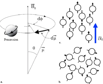
Figure 1.2 a,c. Schematic representation of spinning Hydrogen protons. --- 5

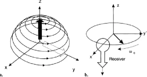
Figure 1.3 Scheme of the magnetization vector viewed from a direction parallel to the static magnetic field after the application of a RF field with frequency of ω0.--- 6

Figure 1.4 a. Excitation of the magnetization when observed in the laboratory frame. --- 7

Figure 1.5 Schematic illustration of the process of the effect of the magnetic field inhomogeneities and how they reduce the Free Induction Decay (FID) and how the application of 180º RF allows for a reduction off this decay effect.--- 8

Figure 1.6 a. Selection of a slice with a gradient field defining the frequency band f1-f2 of said selection. b. Frequency spectrum of the RF pulse. c. Envelope of amplitude of the excitation on time. d. Excitation pulse with following refocussing gradient. --- 9

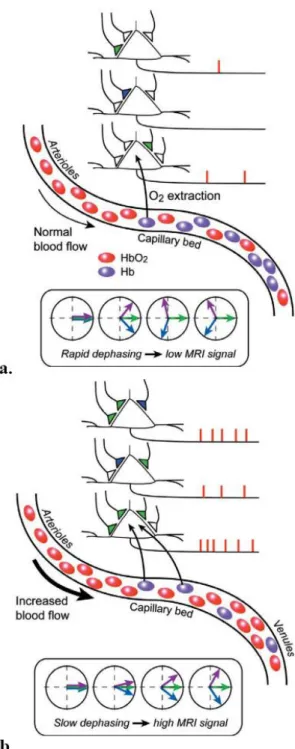
Figure 1.7 a,b. Schematic from neural activity to BOLD MRI response. ---12

Figure 1.8. Idealized time course of the hemodynamic response following a long stimulus (around twenty seconds). ---13

Figure 1.9: Pulse sequence diagram for EPI. ---15

Figure 1.10: Example of a zig-zag traversal of the κ-space in one of the early EPI techniques. ---15

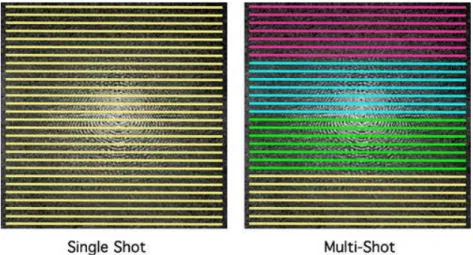
Figure 1.11: Representation of the difference between the single shot EPI sequence. ---16

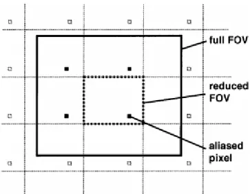
Figure 1.12: Aliasing in 2D Cartesian sampling. ---17

Figure 1.13: Layer and column as core functional parts of the visual cortex. ---18

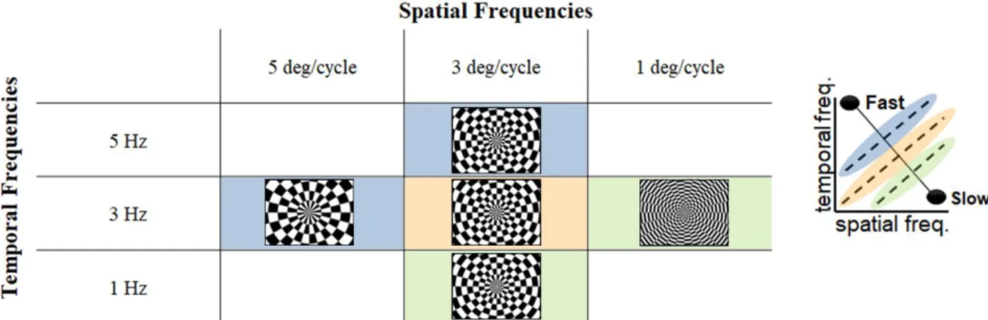
Figure 2.1: Graphical summary of the visual stimuli. ---21

Figure 2.2: Projection of the localizer scan on the anatomical T1 scan, representing the coverage of the former. ---21

Figure 2.3: Projection of the anatomical T2*w scan on the anatomical T1 scan, representing the coverage of the former. ---22

Figure 2.4 a. Representative frames of the localizer task in their several variations: dartboard with moving left side of the visual field, full movement of dartboard, dartboard with moving right side of the visual field. b. Schematic representation of the task with 20 second rest periods and 10 seconds of task. The task periods follow a set-up order of full dartboard movement, left-side moving dartboard and right-side moving dartboard in a total of 360 seconds of task overall (cycled is repeated four times). ---22

Figure 2.5: Projection of the EPI runs on the anatomical T1 scan, representing the coverage of the former. Scans are not aligned. ---23

xii

Figure 2.6 a. Representative frames of the several runs present in the task consisting of high-contrast

black-and-white dartboards with spatial frequencies of 1, 3 and 5 deg/cycle. For the dartboard with spatial frequency of 3 deg/cycle the temporal frequencies were 1, 3 and 5 Hz randomly interleaved and for the 5 and 1 deg/cycle dartboards the temporal frequencies were, on both, 3 Hz. b. Schematic representation of the Event-related design task with stimulus events lasting 1s and with variating resting time intervals, comprising in total 360 seconds. ---23

Figure 2.7: Slice time correction of a functional dataset. During the slice scan time correction, slices

within each functional volume (the black triangles) are shifted in time resulting in a new resampling time series (violet rectangles). In this new time series, all slices of a functional volume are virtually measured at the same moment in time. To calculate the intensity values of the time points that fall in between measurement time points, past and future values were integrated using a sinc interpolation. Here, five slices are scanned in interleaved order.---25

Figure 2.8: Schematic representation of the Least square fits (in red) of the detrending method

(polynomial fit) applied in both the Localizer and Run datasets. Adapted from [54].---25

Figure 2.9: Example of the matricial model for estimating hemodynamic responses by the

deconvolution approach used in the runs. For simplicity, each estimated HRF in this figure is an 8 × 1 vector. For example, the stimulus presentation times are indicated on the right and expressed in volume -TRs (vTR). The stimulus convolution matrix S on the left is constructed based on stimulus presentation times. The HRFs are estimated by solving H = (STS)-1STB. Courtesy of [59]. ---30

Figure 3.1: Representation of the registration parameters (from top to bottom: difference in the

anterior-posterior, right-left, inferior-superior directions and yaw, pitch, roll angles) upon performing a motion correction using Fourier interpolation on one of the localizer scans. These parameters were saved to be used later during the GLM Analysis. All scans, both localizer and run scans, were aligned to their fifth volume of the series. ---32

Figure 3.2: Example of the removal of physiological artefacts by using RETROICOR. In the chosen

voxel, indicated by the green selection axis, the time series were corrected from their original state (in black) to physiological effect free ones (in red). ---33

Figure 3.3 a c: Detrending of motion corrected (and time slice corrected localizer) scans by a linear

least squares detrend. Top left represents a coronal slice, top right a sagittal slice and bottom an axial slice. a. The scan was orthogonalized with respect to two-degree polynomial functions (a sine and cosine wave) with variable period depending on the type of scan: 200 and 195, respectfully, for run scans and 428 and 429, respectfully, for Localizer scans. b. Before the detrending, all the mean intensity values per voxel maps of every scan were generated. c. The mean intensity value per voxel maps calculated in b. were combined with the detrended images to continue the pre-processing analysis. ---33

Figure 3.4: Outlier count of 200 volumes in a localizer scan. The volumes where the outlier count went

beyond the threshold (in red) of several orders of magnitude (1.4 × 104) were removed from the proceeding GLM analysis. ---34

Figure 3.5 a b. Thresholded t-value activation maps of the localizer task visualized with a Bonferroni

corrected threshold p-value of 0.05. These maps are being overlayed in coronal (top), axial (bottom) and sagittal (right) slices of the acquisition. ---34

xiii

Figure 3.6: Representation of clusters of at least 20 voxels of the activation maps (P < 0.05, Bonferroni corrected) from the localizer scan acquisition overlayed in coronal (top) and axial (bottom) slices of the acquisition. These serve as left and right hMT+ activity ROIs for further BOLD analysis. ---35

Figure 3.7: Superimposition of the acquired sagittal (left) and axial (right) run scans on the localizer

scans. From this alignment the transformation matrix required to go from localizer space to run space was obtained allowing the generated ROIs to be put into run space for further analysis without any interpolation of the later images. ---35

Figure 3.8 a b. HRF extraction of one of the runs acquired from one of the subjects. a. These three non

thresholded t-value run activation maps are overlayed on axial slices of the acquisition. These demonstrate that the ROI generated by the localizer scan of this subject (black lines) falls over the region of the activation maps with the highest activation probability (darkest colours represent near to no activation while bright yellow and white represent highest activation). b. The time series of the acquisition (top), the extracted HRF curve of a selected voxel (bottom left) and the mean extracted HRF curve of the whole ROI (bottom right) were plotted for control purposes. ---36

Figure 3.9: Mean HFR extraction for one of the subjects of the study (V4528) of the left hMT+. All the

runs are colour coded (blue for 3 deg/cycle, 1 Hz; red for 3 deg/cycle, 3 Hz; green for 3 deg/cycle, 5 Hz; black for 1 deg/cycle, 3 Hz and light blue for 3 deg/cycle, 1 Hz) and the hemodynamic response signal change in percentage can be seen for about 20 seconds. ---37

Figure 3.10: Mean HFR extraction for one of the subjects of the study (V4528) of the right hMT+. All the runs are colour coded (blue for 3 deg/cycle, 1 Hz; red for 3 deg/cycle, 3 Hz; green for 3 deg/cycle, 5 Hz; black for 1 deg/cycle, 3 Hz and light blue for 3 deg/cycle, 1 Hz) and the hemodynamic response signal change in percentage can be seen for about 20 seconds. ---38

Figure 3.11: Maximum amplitude of the HRF response of both left (to the left) and right (to the right)

hemispheres of one of the subjects in the study. All the differences are indicated with the curly brackets and are of at least one standard deviation. ---38

Figure 3.12: Maximum amplitude of the HRF response of the left hemisphere’s hMT+ for all the

subjects in the study. ---39

Figure 3.13: Maximum amplitude of the HRF response of the right hemisphere’s hMT+ for all the

subjects in the study. ---40

Figure 3.14: Voxel-by-voxel analysis of subject V4528. Voxels with the highest amplitude of HFR on

a specific run are coloured with the colour code of said run and represented on an inflated brain surface generated by their T1 scan (on top). Both left (top left) and right (top right) hemispheres are represented.

A voxel count was performed to infer on the tuning of the hMT+ for speed components on both the left hemisphere (in the middle) and right hemisphere (in the bottom). Here it is also possible to see the colour code for the brain surface representation: red – 1 deg/cycle, 3Hz; blue – 3 deg/cycle, 1 Hz; green – 3 deg/cycle, 3 Hz; yellow – 3 deg/cycle, 5 Hz; purple – 5 deg/cycle, 3 Hz. ---41

Figure 3.15: Voxel-by-voxel analysis of subject V5069. Voxels with the highest amplitude of HFR on

a specific run are coloured with the colour code of said run and represented on an inflated brain surface generated by their T1 scan (on top). Both left (top left) and right (top right) hemispheres are represented.

A voxel count was performed to infer on the tuning of the hMT+ for speed components on both the left hemisphere (in the middle) and right hemisphere (in the bottom). Here it is also possible to see the colour

xiv

code for the brain surface representation: red – 1 deg/cycle, 3Hz; blue – 3 deg/cycle, 1 Hz; green – 3 deg/cycle, 3 Hz; yellow – 3 deg/cycle, 5 Hz; purple – 5 deg/cycle, 3 Hz. ---42

xv

List of tables

Table 3.1: Summary of the visual stimuli (high-contrast black-and-white dartboard) presented during

the several runs of the study. Each run gains a designation in respect to the spatiotemporal frequency of the dartboard presented as stimuli on said run. ---37

Table 3.2: Table with the recollection of significant differences in the maximum amplitude of the HRF

responses of the runs with the dartboard speed of 3 deg/sec, generated with different spatiotemporal frequency combinations (3 deg/cycle, 1 Hz and 1 deg/cycle, 3 Hz). The differences were seen in both hemispheres with a total difference of responses for the same speed in seven of the 10 brain hemispheres present in the study. ---39

Table 3.3: Table with the recollection of significant differences in the maximum amplitude of the HRF

responses of the runs with the dartboard speed of 15 deg/sec, generated with different spatiotemporal frequency combinations (5 deg/cycle, 1 Hz and 1 deg/cycle, 5 Hz). The differences were seen in both hemispheres with a total difference of responses for the same speed in five of the 10 brain hemispheres present in the study. ---39

1

1- Introduction

Even though the perception of speed of a moving object and all the tasks associated with it were identified in several areas of the brain as stated in numerous studies in the past [1]–[6], the general agreement is that the core region responsible for visual motion processing in primates, including humans, is the middle temporal cortex (referred as hMT+ in humans and V5/MT in macaque monkeys and owl monkeys, respectively). Such is demonstrated several times in the several anatomical and functional studies regarding the hMT+ [5], [7], [16], [17], [8]–[15]. While extensive studies have been carried out in the MT due to its retinotopic properties and selectivity for direction of moving stimuli, only recently there was an increase of interest in the mechanism of speed of motion encoding in MT neurons.

This mechanism helps individuals in their spatial navigation, by providing the ability to promptly react to the sudden appearance of potential obstacles or dangers, which in turn leads to the conclusion that any added knowledge behind this complex mechanism holds great potential to help further develop well appropriate solutions for patients who’ve had any damage on the localized brain region of the middle temporal cortex. Findings report the co-existence of an alternative direct route linking the lateral geniculate nucleus (LGN) to the hMT+, bypassing the V1, which serves as an example of the fundamental role played by the hMT+ , even in the presence of individuals with severe destruction of primary visual cortex (blindsight) [18].

The following Subchapter 1.3 of this chapter will subtly dip into the details on these studies and the several advancements that brought attention to this area of the brain as the responsible for encoding the speed of motion in human beings.

Out of the plethora of studies regarding the MT, it is possible to outline two distinct speed encoding mechanisms: the first suggests that the MT neurons have a separate and independent tuning for the spatial and/or temporal frequencies of visual stimuli; the second proposes direct speed tuning, rather than its separation in the two frequencies components.

The two methods (graphically represented in Figure 1.1) provide different predictions about the tuning profiles for spatial and temporal frequencies in the MT neurons. While the direct speed tuning will predict the same preferred speed, given by all the possible combinations of spatial and temporal frequencies; the separated and independent tuning predicts a preferred representation of the speed components (being it either spatial or temporal) instead of the speed per se.

Figure 1.1: Representation of the two paradigms that define speed encoding in the hM T+. a. Several combinations of spatial

and temporal frequency, resulting in the same speed, show similar response, indicating a speed focused tuning profile. b. Response is dependent on spatial or temporal frequency, meaning that different combinations of the two parameters result in different responses.

2

At best, the results that came from countless animal physiology studies can be considered conflicting. While some report that macaque have a more than half of the middle temporal visual area cells tuned for speed [19], with these results being comparable with other reports [20]; others report, for example, in single neuron recordings done in nonhuman primates and also marmosets, to a majority of neurons with distinct responses for spatial and temporal frequencies and only a small percentage displaying a speed tuning profile [21]–[23].

Regarding the human homologue of MT/V5, the studies about responses to speed of motion in the hMT+ come with the same degree of uncertainty present in the animal physiology studies. It is still unsure if the neuronal tuning in human MT+ reflects speed tuning, independent spatial and temporal frequency tuning, or even perhaps a combination of both.

Traditionally, the experiments performed towards a better understanding of speed encoding in the human MT+ were done using functional magnetic resonance imaging (fMRI), magnetoencephalographic (MEG) neuronal responses and intracranial electrocorticography (ECoG). In these, the most widely used motion stimuli were broadband stimuli such as random dots of even spots of light [24]–[26] and its broadband nature doesn’t allow for a clear distinction in between speed tuning of independent spatiotemporal frequency tuning. Also, by observing studies that used gratings moving at different speeds to infer about the encoding of speed motion, only an fMRI adaptation experiment using drifting gratings [27] provided evidence of speed tuning of Blood-oxygen-level dependent imaging (BOLD) responses over different temporal frequencies conversely to the results gathered by MEG [28], which showed independent spatial and temporal frequency tuning in response to said gratings in hMT+.

This thesis comes as a follow up of the work done by Gaglianese, A et al [29], where ECoG was used to investigate speed tuning properties in hMT+ neuronal populations in response to visual motion stimuli. Its findings pointed to neuronal population response to the spatiotemporal frequency properties and not the speed per se of the stimuli, consolidating and extending the findings in macaque and marmoset MT neurons to the now human neuronal populations present in the MT. Here fMRI was found to be the missing link and a valuable addition to corroborate these past results. By combining this non-invasive technique and the extraordinary resolution power of 7T, while extending the findings to a healthy subject dataset, the knowledge of how the hMT+ encodes speed motion would come naturally to light. Also, the proven matching between BOLD and neuronal activity at a scale of mm [30] will also provide proof on the ECoG findings.

The objective is to understand whether the response preferences of the neural populations present in the hMT+ depend on the stimulus speed or the independent spatial and temporal frequency components. More so, the high spatial resolution of the 7T will allow for the division and clustering of neuronal populations inside the MT that exhibit separate and independent spatial and temporal frequency or conversely the stimulus speed directly, with selectivity to multiple combinations of its frequency components.

These findings may point to a division of the human MT+ complex into sub regions [24] that may be identified as homologs to a pair of macaque motion-responsive visual areas, middle temporal visual area (MT) and the medial superior temporal area (MST), with their neuronal populations encoding speed in the two different established methods, explaining the unclearness behind speed encoding in the hMT+.

3

1.1. Project Specifications and Goals

The vast infrastructures and clinical possibilities present in the Utrecht University Medical Centre (UMCU) research environment allowed for the setup of the experiments that this thesis revolves around. Having vast access to patient data who underwent implantation of ECoG grids for the purpose of epilepsy monitoring gave birth to a novel study that used ECoG, a technique with recent increased interest due to its direct and high temporal and spatial resolution measure of neuronal activity within relatively small neuronal populations in the human brain, as means to investigate the speed tuning properties in response to square-wave dartboard moving with several temporal and spatial frequency combinations. [29] Also the sheer power of the high-field 7T fMRI and the high spatial resolution achieved by the development of high spatial resolution surface coils [31] allowed a signal-to-noise ratio level that allowed the study to be performed. The combination of these last two events make the UMCU one of the few neuroimaging centers in the world that allows the mapping of the visual cortex in a non-invasively way under the millimetre scale. By gathering all conditions, the experiment serves as a bridge in between the several neuron recordings done in non-human primates and non-invasive methods such as MEG, Electroencephalography (EEG) and even fMRI studies in humans.

Part of the fMRI studies on humans were traditionally done with main usage of broadband stimuli [25], [26], [32], like random spots of light and/or random dots, as motion stimuli to investigate speed responses. The nature of these broadband stimuli doesn’t allow for distinction between speed tuning or independent spatiotemporal frequency tuning. Although, by using and focusing on adaptation of drifting gratings in an fMRI experiment performed in humans, evidence was provided in the direction of speed tuning of BOLD responses over several temporal frequencies [27].

The final link stands in the methodological use of stimuli that provoke robust responses, like random dot motion patterns and square-wave checker boards, with independent manipulation of temporal and spatial frequencies for a proper analysis of the hypothesis of these components being part of the speed encoding mechanism. Thus, a conclusion was drawn: square-wave checkerboards would be the appropriate stimuli for this type of study. Conversely to the what is expected, checkerboard stimuli hard edges with contrast energy at multiple spatial and temporal frequency harmonics are still regarded as exhibiting a single speed, that being the one of the change in edge position per second. [29]

In combination with the usage of the Philips 7T scanner with the help of two 16-channel high-density multi-element surface coil with minimal electronics developed and present at the UMC and the 16-channel [31], the high contrast potential and accuracy for most of the human tissues brought by this magnitude of B0 strength with the close proximity to the head allowed by the high-density multi-element surface coil allows us to draw some conclusions, contributing to in the definition of a pattern for the speed encoding in the hMT+. Since fMRI is a non-invasive technique and there is a strong positive correlation link between the BOLD amplitude and the ECoG broadband power in some areas of the brain [30] the present study will corroborate or refute some of the conclusions drawn previously in [29], while also expanding them to a healthy population.

4

1.2. Background

1.2.1. Magnetic Resonance Imaging and functional Magnetic Resonance

Imaging

Magnetic resonance imaging (MRI) is a medical imaging technique rapidly with a galloping increasing interest due to its excellent contrast potential and accuracy provided for most of the tissues present in the human. The technique has already existed for more than thirty years, with a lot of its improvements and developments being achieved as higher resolution, better contrast techniques as well as improved safety mechanisms and potential long-term effects analysis. [33]–[35]

The technique allows for visualization of both anatomical and functional data of the human brain and, broadly speaking, it was birthed in the behavior of the magnetization vector of a specific set of protons precessing after being excited by a controlled radiofrequency pulses. [36]

Functional magnetic resonance imaging (fMRI) has grown to be the most widely used tool to study neuronal activity in the human brain in vivo with its oxygenation level-dependent signal ever since it was discovered twenty years ago with a setup of magnetic resonance imaging that allowed for the reception of level of oxygenation signals [37].

The spatial and temporal resolution provided by state-of-the-art MR technology with its non-invasive character, allowing for multiple studies to be performed in the same subject, grant huge advantages to fMRI over the other functional neuroimaging techniques, like positron emission tomography (PET), which are also based on changes in blood flow and cortical metabolism.

Basic principles and methodology of fMRI are explained during this chapter, as well an extensive description of the BOLD contrast mechanism physiology, after a brief description of the physical fundamentals of MRI at a conceptual level.

1.2.2. Physical Principles of MRI

Physical principles of MRI are shared for anatomical and functional imaging. We can split the operation of MRI in two major themes: excitation and recording of electromagnetic signal (reflecting the properties of the measured object), and construction of two- and three-dimensional images (reflecting on how its measured proprieties vary throughout space).

1.2.2.1. Spin Excitation and Signal Reception

The core of spin excitation resides on the magnetic excitation of body tissue and the reception of returned electromagnetic signals from said tissue. All nuclei with an odd number of protons are considered magnetically excitable and while it can happen within all the magnetically excitable nuclei, MRI focuses on the most common isotope of hydrogen with a nucleus of only one proton. Hydrogen protons (1_{H) are ideally suited for MRI due to their abundance in human tissue and favorable magnetic}

properties.

It is the spin that provides the magnetic properties to protons, and due to that, the rotation like a spin top around their own axes, a small directed magnetic field is inducted (Figure 1.2a).

5

Figure 1.2 a,c. Schematic representation of spinning Hydrogen protons. a. Representation of the circular motion of the axis of

rotation of a spinning body, in this case hydrogen protons, around another fixed axis, (B0), produced by a torque applied in the

direction of the motion; defined as precession. b. Whenever no external magnetic field is present, the direction of the spin is distributed in a random manner. c. Upon the presence of an external magnetic field, the affect ed spins will align either parallelly or antiparallelly . Ultimately this results in a net magnetic field parallel to the external magnetic field due to the predominance of parallelly aligned spins. Adapted from [38].

In a normal environment, the collection of all magnetic fields created by the spins in the human body would be oriented randomly, thus canceling each other out (Figure 1.2b). However, when placed under the effect of a strong static magnetic field (B0) of an MRI tomograph, the spins within the subject will orient themselves in line with the present field.

This alignment can either be with the field (parallel to it) or against the field (antiparallel to it) (Figure 1.2c). It is to note that the said “alignment” is but an abuse of language since there is no alignment of rotation axis but of movement of rotation around the direction of the scanner static magnetic field: this motion is called precession. The two states of precession differ in the energy their protons carry, with the parallel precession having less energy and thus being more stable. Due to this difference of energy, a higher percentage of parallel protons are found in the volume, causing the body to be magnetized.

1.2.2.2. From Larmor Frequency and Equation to Resonance

The excess number of spins will produce a total excess magnetic field called M0. The precession frequency of the protons that produce this field depends on the strength of the surrounding magnetic field. More precisely, the precession frequency 𝜔0 is directly proportional to the strength of the external

magnetic field and is defined by the Larmor Equation:

𝜔0= 𝛾𝐵0 (1.1)

The symbol of 𝜔0 is known as the precessional, Larmor or resonance frequency. The symbol 𝛾

refers to the gyromagnetic ratio, which is a constant unique to every atom (for hydrogen protons this is 42.56 mHz per Tesla [33]).

6

When an electromagnetic pulse with the same frequency as the proton’s precession frequency is applied to the protons present in the volume, these will absorb the transmitted energy, getting excited in the process. This principle is the basis of the imaging technique and it gives the name to it: Resonance. Since the precession frequency is in the range of the radio frequency (RF) waves, the electromagnetic pulse can be called radio frequency pulse.

As an effect of being excited, all the spins that were in the parallel state (associated with a lower energy level) will then absorb the energy and to go the anti-parallel state (associated with a higher energy level) and will start precessing in phase. This phased precession will cause the magnetization vector M0

to start moving down towards the x-y plane. This plane is perpendicular to the static magnetic field and, thereby goes by the name of transverse plane. The angle between the magnetization vector and the transverse plane is referred as α and is one of the means of characterization of RF pulse strength and duration.

When α is 90º, the magnetization vector is completely within the transverse plane, meaning that, in terms of proton alignment, the number of protons aligned parallelly and antiparallelly is equal (Figure

1.3). The added spins form a net magnetic field called MXY which exists in the transverse plane and can

be measured in the receiver coil since it induces a detectable current flow.

Due to the nature of the RF pulse, right after its end, the phasing existent within the precessing protons will also cease to exist, due to the spin-spin interactions of the magnetic fields, which ultimately cause the decay of the transverse magnetization in a few tenths of a millisecond.

Figure 1.3 Scheme of the magnetization vector viewed from a direction parallel to the static magnetic field after the application

of a RF field with frequency of 𝜔0. Courtesy of [39].

The transverse dephasing is a result of the interaction between spins. Such interactions lead to slightly different local magnetic field strengths. In turn, these local magnetic field differences lead to different precession frequencies and thus phase shifts between precessing spins. This process is called dephasing and since it happens in the transverse plane it can also be called transversal relaxation and it evolves over time following an exponential function with time constant of T2. This relaxation isn’t

represented by the T2, but by its successor, T2*, which accounts for the faster dephasing of the spins due

to the differences in the inhomogeneities of the static magnetic field and in the physiological tissue as well. Therefore, the raw signal measured in the receiver coil, also called free induction decay (FID), will decay with the shorter time constant T2*.

𝑀𝑋𝑌= 𝑀0𝑒 𝑡

𝑇2∗

⁄

(1.2)

These local field inhomogeneities causing the different precession frequencies that in the end increase the speed of the dephasing allows fMRI to exist as a technique since those field inhomogeneities

7

have a dependency in the local physiological state, i.e., state of local blood oxygenation and level of local neuronal activity, and the measurements of these field changes will allow the inference of neuronal activity. More details on this and their importance in the fMRI technique will be discussed in the following subchapter 1.1.2.

Figure 1.4 a. Excitation of the magnetization when observed in the laboratory frame. b. The presence of a current loop

(sensitive for transverse magnetization) close to the changing magnetic flux of the rotating magnetization causes an induced current: the M R signal. Adapted from [39].

Two effects affect the spin’s speed of dephasing: random effects as well as fixed effects caused by magnetic field inhomogeneities. The field inhomogeneities’ dephasing effect can be reversed with the application of a 180º RF pulse. By allowing 𝑡 = 𝜏 to elapse before the application of a reversing RF pulse, the dephased spins will flip on their X’ and Y’ relative rotation axis, allowing them to reverse their order while maintaining their direction of rotation. Due to the application of the 180º RF pulses, at a time of 𝑡 = 𝑇𝐸 = 2𝜏 the vectors will be again back in phase producing a large signal that goes by the name of spin echo.

This amplitude of the obtained spin echo is smaller than the amplitude of the initial FID. This is due to the spin-spin interactions that inevitable produces irrecuperable loss of signal (during T2 decay).

This goes in a circle by applying consequent 180º RF pulses, since all the spins can start going out of phase the moment that they are back in phase at the echo time. The process can be repeated for as long as enough signal is available, with the interesting part of the process being the possible selection of the T2 signal amplitude by the correct setting of the timing on the 180º pulses (Figure 1.5).

Spins also reorient themselves with the direction of the strong magnetic field that is provided by the scanner while going back to the low energy state after being excited. Longitudinal relaxation is the designation of this spin reorientation with the external magnetic field and it happens to be a slower process than the previous discussed dephasing. The longitudinal component Mz will suffer a recovery

dictated by an exponential function with a time constant T1:

𝑀𝑍= 𝑀0(1 − 𝑒 𝑡

𝑇1

⁄ ₎

(1.3) It is important to notice that the absorbed energy provided by the RF pulse is released both in a way to be detected outside of the body as RF waves; and some part is released to the nearby surrounding tissue, being designated by the term lattice. Just like interactions between spin-spin determined T2 and,

consequently, T2*, the interactions spin-lattice will determine the speed of T1 recovery. What this

represents is that T1 is tissue-specific, and with this value and T2, MRI allows for a differentiation

8

Figure 1.5 Schematic illustration of the process of the effect of the magnetic field inhomogeneities and how they reduce the

Free Induction Decay (FID) and how the application of 180º RF allows for a reduction off this decay effect. The three representations of coloured spin vectors precessing at resonance frequency, slightly faster and slightly slow er than that (green, violet and blue vectors, respectively). The 180º RF pulse flips the dephased vectors about the X’ axis, reversing the order of the spins but not their direction of rotation. This flip culminates in the vectors falling back in phase which induces a large signal called spin echo. The time from the application of the 180 RF pulse and the spin echo is called echo time (TE). Adapted from [40].

1.2.2.3. Image reconstruction: Slice selection, Frequency and Phase

encoding

The principles of magnetic resonance may provide some insights on the physical effects behind the technique but by themselves they solely are not representative on how it is possible to obtain images of human tissue. To put it into perspective: up to this moment the insight on the magnetic resonance Imaging provided was focused only on the magnetic resonance portion; from now on we discuss the Imaging.

To convert the signals obtained from the excitation of protons into a cohesive image there’s a very important step to be taken: assigning components of the signal to its originated positions in space. Not all sequences have the same processes behind them, but the localization of signal source has the combined action of three fundamental techniques: selective excitation of a specific slice; phase and frequency encoding. Three fundamental techniques for three fundamental dimensions, allowing for a complete spatial localization of the received signal.

By analyzing the Larmor equation (1.1), the knowledge that spins exposed to a higher magnetic field will precess faster comes clear to us. This, coupled with the usage of magnetic field gradients created by the gradient coils of the MRI scanner, will add this new magnetic field to the static one existing beforehand. The field strength will then vary linearly with the distance from the magnet’s center. In conclusion, spins exposed to the side of higher magnetic field precess faster, while spins exposed to the side of the lower magnetic field will precess slower.

With RF pulses with frequencies within specific bands, a slice of the imaged object will be excited selectively and any spins that fall outside of that range that are precesing at a different speed won’t absorb the RF transmitted energy (Figure 1.6a).

Slice orientation will always be performed perpendicularly to the axis of the gradient (z-axis), or, by other words, an axial slice will be the result of this slice selection. With the same logic we get to

9

the conclusion that a gradient along the x-axis produces a sagittal slice selection and along the y-axis a coronal slice selection. Oblique slices fall out of these simple rules, but the general approach is their selection by application of simultaneous gradients combination.

Figure 1.6 a. Selection of a slice with a gradient field defining the frequency band f1-f2 of said selection. b. Frequency spectrum

of the RF pulse. c. Envelope of amplitude of the excitation on time. d. Excitation pulse with following refocussing gradient.

The slope of the applied gradient and the frequency band of the applied RF will influence the position and thickness of the selected slice.

After this slice excitation, the echo that is measured is restricted to a compound signal from the protons within said slice and for the rest of the spatial encoding the slice selection gradient is turned off. Following the slice selection, a second gradient can be applied along one of the two remaining spatial dimensions while receiving the signal from said excited slice. This is the basis of what is called frequency encoding.

By having this second gradient running along one of the other spatial dimensions, the protons within the slide will precess with different frequencies along the respective dimension, which in turn will allow for a differentiation in their spatial position in the received signal.

The gradient applied during frequency encoding is usually designated as the read-out gradient due to being tuned on during reception of the signal coming from the protons. The strength of the signal at each frequency is dependent of the strength of the signal at the specific encoded position.

The sum of all frequency responses will obviously consist of all the measured composite time domain signal. This information allows us to use the Fourier transform (FT) to obtain from the composite signal, the strength of the signal at each specific frequency. By other words, the FT provides the frequency-specific information of the signal that, in the end, merely represents the spatial information required to form an image. The image formed with the frequency-specific information uses a grey level to represent the strength of the signal at each picture element.

Even if, at this point, we’re able to recreate an image from all the magnetic information received, one further step is required to be able to separate signal components origination from different positions along the second dimension in the imaging plane. By briefly adding an extra gradient in the static magnetic field with an orientation along the remaining (third) spatial dimension it is possible to phase encode the signal before its reception. The phase encoding merely consists of a slight change in the precession frequency in each row of the slice caused prior to the read-out. The affected protons within each row will precess with a systematic phase shift along the positions on said row after the phase

10

encoding gradient is turned off. The amount of phase shift will depend on the position of the proton in along the encoded second image dimension.

The phase encoding gradient is turned off a moment before the echo read-out as its existence would cause an ambiguous spatial encoding if coupled with the frequency encoding gradient. The two gradients coexistence on the receiving of the echo would result in two-dimension frequency encoding gradients and thus, ambiguous spatial encoding. In the end would represent two different spatial positions being coded in a similar way, much like different numbers can be added to represent the same number.

Through proper combination of both frequency encoding in one dimension and phase encoding in the remaining dimension, all positions within a 2D image (or slice) can be uniquely coded with a determined resolution.

This is, though, without lack of a flaw: the phase-encoding gradient by its own is not sufficient to encode the second image dimension without being repeated many times for a single slice . The repetitions alter in the strength of the phase-encoding in order to, ultimately, obtain a complete phase and frequency encoding of the selected slice.

1.2.2.4. Two-dimensional κ-space and the formation of the 2D

Echo-Planar Images

All the procedures, if applied correctly, will provide a set of data resultant from the series of excitation-recording. This data is then arranged into a two-dimensional space, in frequency space, designated κ-space. Each row of the κ-space corresponds to the data gathered by one cycle of the excitation-recording cycle with different phase-encoding gradient strength. While the slice selection and frequency encoding gradients are constant throughout cycle to cycle, the slope of the phase encoding gradients changes constantly by a set amount from cycle to cycle. This imposed shift for a specific Hydrogen proton depends on the strength of the phase encoding gradient and position of the proton along the second image dimension.

κ-space is then filled in such a way that the second slice dimension also gets frequency encoded. The κ-space contains then two-dimensional frequency encoded information of the slice, which then is transformed into two-dimensional image space by the application of the two-dimensional Fourier transform (2D FT).

This procedure is applied for each slice of a scanned volume. In order to construct a single or multiple 2D images from electromagnetic echoes, a particular sequence of electromagnetic pulses must be applied. These sequences are given the name of MRI pulse sequence and the details of a specific pulse sequence named echo-planar imaging (EPI) will be given in Subchapter 1.2.3.4.

11

1.2.3. Physiological Principles of functional MRI

The MR images and the techniques used for their acquisition have been perfected throughout the years to describe at its best possible a plethora of biological tissues’ properties. Even though MRI is heavily used for its structural view of, for example, the brain matter; to map functional changes in this organ and to track or trace neuronal activity, MRI requires an extension of its approach through time.

This concept is the basis of functional magnetic resonance (fMRI) and the focus of this subchapter. It may seem like fMRI is simply the study of the fluctuation and differences in time of the magnetic properties between arterial blood (oxygenated) and venous blood (deoxygenated), the details and caveats of these types of studies, the processing and interpretation of the data involved are enough to form a distinct field of study.

1.2.3.1. Neurovascular Coupling and The BOLD effect

The existence of neuronal activity is one that requires a constant consumption of energy. Said energy is produced via chemical processes that require the presence of glucose and oxygen which are supplied by the complex vascular network of small and large vessels. Oxygen is transported in the blood via the hemoglobin molecule. Hemoglobin is a molecule that can have two times of terminology associated depending of the presence of oxygen: if the hemoglobin present in the vessels is carrying blood, it is designated oxygenated hemoglobin (HbO2); if this is not the case it is called deoxygenated

hemoglobin (Hb).

When talking about the arterial part of the vascular system, we see a transport of oxygenated blood through an increasingly fine-grained network of blood vessels until its dimensions allow for a chemical transfer of the stored energy (oxygen) to the neurons.

In the brain’s resting state only 30 to 40% of the oxygen present in the blood of the capillary bed is extracted. Both the capillary bed and the venous network contain a mixture of oxygenated and deoxygenated hemoglobin. Due to this the venous system, counterpart to the arterial system, performs the transportation of the less oxygenated blood away from the capillary bed to the pulmonary system, thus completing the cycle of blood transportation back to where the blood oxygenation takes place.

There is a local increase of neuronal activity, because of the frequent neuron firings happening in the brain. This event increases the oxygen extraction rate in the capillary bed which, in turn, will increase the relative concentration of deoxygenated hemoglobin.

12 The vascular system response to the increased energy demand is designated as hemodynamic response. The hemodynamic response is characterized in the local increment of cerebral blood flow (CBF), delayed approximately one to two seconds, and the cerebral blood volume (CBV), due to an increase of the size of vessels. The combined interplay between oxygen extraction, CBV and CBF results in what is classified as the hemodynamic response function (HRF), which is no less than the time course of evoked fMRI signals during an activation of a brain region.

While the HRF has a plethora of physiological events happening in the three phases that it consists of, it is important first to understand the underlying physical properties of the blood and how the MRI becomes sensible to measure these effects due to what is called the BOLD.

Oxygenated hemoglobin has different magnetic properties than deoxygenated hemoglobin, more specifically, while the first is diamagnetic the second is paramagnetic and thus alters the local magnetic susceptibility and inducing magnetic field distortions within and around blood vessels in the capillary bed and venules. During the mentioned oversupply phase of the hemodynamic response, the oxygenated to deoxygenated hemoglobin ratio increases, resulting in a more homogeneous local magnetic field. This homogeneity causes the spins dephasing to happen slower, or in other words, the measured MRI signal in homogeneous magnetic fields is stronger, which leads to the association between the activated brain states and higher measured MRI signals while compared to the resting states. The BOLD effect measures increased neuronal activity indirectly via the local changes in magnetic field (in)homogeneity, caused by oversupply of oxygenated blood following the neuronal activation (Figure 1.7). This effect is the most common primary form of fMRI contrast, discovered by Ogawa, S. [37], being detectable with MRI due to the different magnetic properties of oxygenated and deoxygenated hemoglobin, acting as endogenous marker of neural activity.

As mentioned before, the hemodynamic response function is divided into several phases: initial dip, main response and undershoot. The main response phase of the HRF is dominated by the quick and strong CBF in response to the slightly increased oxygen extraction rate. Because of that, a local substantial oversupply of oxygenated

hemoglobin is originated, and the MRI signal becomes higher due to the homogenization of the magnetic field. While the details of this supply of cerebral blood flow in an overly unnecessary fashion are unclear

Figure 1.7 a,b. Schematic from neural activity to BOLD MRI

response. a Represents the case of a cortical region in baseline mode. Here the neural activity is low, the cerebral blood flow (CBF) is at a basal level and the constant oxygen rate that fuels neuronal activity causes the 1:1 ratio of Hb and HbO2 to

distort the magnetic field, due to Hb presence. b Represents the case of an activated state in a cortical region. This will lead to an increased oxygen extraction rate, CBF strongly increases delivering more local oxy gen beyond local need (overshoot), pushing HbO2 away from capillary bed. Since

HbO2 does not substantially distort the homogeneity of t he