This is a pre-copy-editing, author-produced PDF of an article accepted for publication in Water Resources Research following peer review. The definitive publisher-authenticated version. Monteiro, H. and Roseta-Palma, C. (2011), Pricing for scarcity? An efficiency analysis of increasing block tariffs. Water Resources Research, 47(6): W06510. is available online at:
Pricing for Scarcity? An E¢ ciency Analysis of
1
Increasing Block Tari¤s
2
Henrique Monteiro
Catarina Roseta-Palma
y3
Abstract
4
Water pricing schedules often contain signi…cant nonlinearities, such
5
as the increasing block tari¤ (IBT) structure that is abundantly applied
6
on residential users. IBT are frequently supported as a good tool for
7
achieving the goals of equity, water conservation and revenue
neutral-8
ity but seldom have they been grounded on e¢ ciency justi…cations. In
9
particular, existing literature on water pricing establishes that although
10
e¢ cient schedules will depend on demand and supply characteristics, IBT
11
can hardly ever be recommended.
12
In this paper, we consider whether the explicit inclusion of scarcity
13
considerations can strengthen the appeal of IBT. Results show that when
14
both demand and costs react to climate factors, increasing marginal prices
15
may come about as a response to a combination of water scarcity and
16
customer heterogeneity. We derive testable conditions and then illustrate
17
their application through an estimation of Portuguese residential water
18
demand. We show that the recommended tari¤ schedule hinges crucially
19
on the choice of functional form for demand.
20
JEL classi…cation: C23; C52; D42; Q21; Q25
21
Keywords: water pricing; nonlinear pricing; increasing block tari¤s; water
22
scarcity; residential water demand.
23
henrique.monteiro@iscte.pt. Economics Department and UNIDE, ISCTE-IUL - Lisbon University Institute, Av. das Forças Armadas, 1649-026 Lisboa, PORTUGAL.
ycatarina.roseta@iscte.pt. Economics Department and UNIDE, ISCTE-IUL - Lisbon
1
Introduction
24
In many areas where water is not abundant, water pricing schedules contain
sig-25
ni…cant nonlinearities. Utilities tend to be local natural monopolies, consumers
26
cannot choose multiple connections and resale is tricky. Thus it is easy, and
27
often politically expedient, for utilities to undertake extensive price
discrimina-28
tion, both for distinct types of consumers (residential, industrial, agricultural,
29
and so on) and for di¤erent levels of consumption within each consumer type.
30
Many utilities use two-part tari¤s, with …xed meter charges and a constant unit
31
price, or multipart tari¤s, which combine …xed charges and increasing or, less
32
often, decreasing blocks. Occasionally, seasonal price variations are employed
33
to re‡ect changes in water availability throughout the year. Less common is
34
the imposition of a scarcity surcharge during drought periods, regardless of the
35
season. In extreme droughts water rationing is generally preferred.
36
It seems that the two main motives for water managers’ enduring defense
37
of increasing blocks are their alleged ability to bene…t smaller users and their
38
potential role in signalling scarcity. The lower prices charged for the …rst cubic
39
meters of water are meant to favour lower-income consumers, which use water
40
mainly for essential uses such as drinking, washing, bathing or toilet-‡ushing.
41
The higher prices in the following blocks are set to induce water savings from
42
other users, such as wealthier households with nonessential uses like sprinkling
43
gardens or …lling pools. IBT are thus a form of cross-subsidization, where access
44
to an essential good by poorer users is paid for through the penalization of higher
45
consumptions by the richer. However, if poorer households are larger, due to
46
either larger family size or to the necessity of sharing a meter, increasing prices
47
can end up penalizing the lower-income households they are meant to bene…t
48
(Komives, Foster, Halpern and Wodon (2005)). A third objective that can be
49
achieved through IBT is revenue neutrality (Hanemann (1997)). Although other
50
tari¤ structures could be used to meet this goal, IBT are one way of allowing
51
utilities to break even in a situation of increasing marginal costs, while still
52
using e¢ cient marginal-cost pricing for the upper blocks. One last justi…cation
53
for IBT pointed out in the literature is the positive externality from a public
54
health point of view of a minimum amount of clean water, "reducing the risks of
communicable diseases throughout the community" (Boland and Whittington
56
(2000)), especially in developing countries.
57
Highlighting the link between climate and the use of IBT, Hewitt (2000), p.
58
275, notes that "utilities are more likely to voluntarily adopt ... [IBT] if they
59
are located in climates characterized by some combination of hot, dry, sunny,
60
and lengthy growing season", which is con…rmed by several recent OECD
publi-61
cations (OECD (2009), OECD (2006), OECD (2003)). For instance, in Europe
62
IBT are more common in the Mediterranean countries like Portugal, Spain, Italy,
63
Greece or Turkey. IBT are commonly used by Portuguese water utilities to price
64
residential water consumption, even though tari¤s are independently chosen by
65
each of the more than 300 municipalities. Portuguese residential water tari¤s
66
typically have both a meter charge and a volumetric price, and the latter almost
67
always consists of IBT. More surprisingly, considering the signi…cant seasonal
68
di¤erences in water availability in the country, seasonal price variations are not
69
common, and the few that do exist seem to be uncorrelated with regional climate
70
characteristics. It should also be emphasized that many utilities incorporate a
71
(large) number of further complications into their water rate calculations, such
72
as the implementation of formulas within blocks, the existence of initial blocks
73
with …xed rates or the application of special contracts, so that complexity is
74
de…nitely the prevailing feature of water tari¤s in Portugal. In an attempt to
75
simplify matters, the Regulating Authority for Water and Waste (ERSAR) has
76
included a four-block tari¤ design in its recent proposal for a tari¤ regime to
77
promote e¢ cient water pricing.
78
In contrast, the literature on e¢ cient tari¤ design does not generally
rec-79
ommend increasing price schedules. Only part of the abundant literature on
80
water pricing provides e¢ ciency results, since most studies either compare the
81
properties of di¤erent possible price schemes or estimate water demand, while
82
many also point out the di¢ culties in moving toward more e¢ cient pricing rules.
83
Many important issues, as summarized in the extensive literature review done
84
by Monteiro (2005), are not speci…c to the water sector: marginal cost pricing,
85
capacity constraints, resource scarcity, revenue requirements or nonlinear
pric-86
ing are signi…cant in the more general framework of regulated public utilities,
as is clear from books like Brown and Sibley (1986) and Wilson (1993).
How-88
ever, such issues appear in this sector combined with some of its peculiarities,
89
such as the prevalence of local natural monopolies, the seasonal and stochastic
90
variability of the resource it aims to supply and the essential value of the good
91
for its consumers. Nonetheless, Monteiro (2005) notes that whenever
justi…ca-92
tions for increasing block rates appear, they are not directly related to scarcity
93
concerns. Although in the presence of water scarcity the true cost of water
in-94
creases due to the emergence of a scarcity cost, it is unclear whether increasing
95
block tari¤s are the best way to make consumers understand and respond to
96
water scarcity situations, especially when the resulting tari¤s are very complex.
97
Our contribution in this paper is to investigate whether climate variables
af-98
fect Ramsey price structures, and in particular whether consideration of such
99
variables can contribute to the choice of IBT as an e¢ cient pricing strategy.
100
A recent related reference in the pricing literature is the paper by Elnaboulsi
101
(2009), which includes a climate parameter in consumer utility and looks at the
102
impact of demand and capacity shocks on state-contingent contracts. However,
103
the paper is purely theoretical and it does not evaluate the properties of the
104
derived nonlinear pricing expression, thus steering clear of the debate on IBT.
105
Current analysis of this issue is specially relevant considering that the Water
106
Framework Directive required that by 2010 (art.9, n.1) pricing policies in the
107
European Union’s member states not only recover the costs of the resource
(in-108
cluding environmental and scarcity costs) but also provide adequate incentives
109
for consumers to use water e¢ ciently, contributing to the attainment of
envi-110
ronmental quality targets. The problem of water scarcity in particular is now
111
recognized by European institutions (EEA (2009)) as an increasingly relevant
112
one in the face of potentially more frequent extreme weather events due to
cli-113
mate change, as can be seen in a recent Communication issued on the topic by
114
the European Commission (EC (2007)).
115
We propose di¤erent models of e¢ cient and second-best nonlinear prices
116
under scarcity constraints, and conclude that, when both demand and costs
117
respond to climate factors, increasing marginal prices may indeed come about
118
as a response to a combination of water scarcity and customer heterogeneity
under speci…c conditions, which we derive, although nonlinear pricing is still a
120
consequence of consumer heterogeneity and not explicitly of water scarcity.
Fur-121
thermore, we then test whether those conditions hold in Portugal by estimating
122
the water demand function and analyzing the behavior of its price elasticity.
Un-123
like in previous literature on water demand estimation, special attention is given
124
to the choice of functional form for the water demand equation, as it determines
125
the restrictions on the price-elasticity of demand. We compare the properties
126
of the most widely-used functional forms and test these for Portuguese data.
127
2
Scarcity in a simple model
128
A simple and intuitive view of the main aspects of e¢ ciency in water prices is
129
presented by Gri¢ n (2001) and Gri¢ n (2006). His model includes three pricing
130
components: the volumetric (i.e. per unit) price, the constant meter charge and
131
the one-o¤ connection charge. The latter is meant to re‡ect network expansion
132
costs and will not be considered in our model, since access to water supply
133
networks is nearly universal in Portugal, with 92.3% nationwide connection rates
134
and 100% in urban areas (APA/MAOTDR (2008), INAG/MAOTDR (2008)).
135
Moreover, we focus on the volumetric part of the tari¤, assuming that the
136
…xed charge, if any, is calculated so as to cover exactly the …xed costs of the
137
water supply activity, which is the legally admissible situation in Portugal since
138
the publication of Law 12/2008. On the other hand, Gri¢ n (2001) assumes a
139
single volumetric price and does not allow for more general nonlinear prices.
140
In fact, the author stresses "the ine¢ ciencies of block rate water pricing" (pp.
141
1339 and 1342), most prominently the fact that multiple blocks obscure the
142
marginal price signal. A somewhat di¤erent approach to the issue of water
143
pricing under scarcity is presented by Moncur and Pollock (1988), where water
144
is a nonrenewable resource with a backstop technology. Our model is closer to
145
Gri¢ n (2001), although we develop it further to include nonlinear prices due to
146
customer heterogeneity (whose relevance is pointed out by Krause, Chermak and
147
Brookshire (2003)) and also to analyse the impact of climate variables (Section
148
4).
149
Considering a static model for di¤erent consumer groups, de…ned by their
heterogeneity in relevant variables (see Section 3), with a scarcity constraint,
151
shows that the marginal cost pricing rule still holds. De…ne Bj(wj) as the
152
increasing and concave monetized bene…t of water consumption for consumer
153
group j; with j = 1; :::; J anddBj
dwi = 0 for i 6= j; and C(w) as the (convex) water 154
supply costs, which depend on the total water supplied, i.e. w = PJj=1wj.
155
The assumption that costs are convex in w means that marginal costs increase
156
as more water is supplied, yet we also introduce a direct scarcity constraint to
157
re‡ect ecosystem limits on water abstraction. In particular, we assume there
158
is a limit to water availability, with the maximum amount denoted as W: The
159
welfare maximization problem is
160 M ax fwjg J P j=1 Bj(wj) C(w) s:t: J P j=1 wj W (1)
resulting in …rst order conditions dBj dwj =dC dw + 8j (2) J P j=1 wj W; 0; (W J P j=1 wj) = 0 (3)
where is the Lagrangian multiplier and it is assumed that all wj are positive (every consumer requires a minimum amount of water). The e¢ ciency result, expressed in equation (2), indicates that the marginal bene…t of water consump-tion should be equal to long-run marginal costs (including scarcity costs if the constraint is binding). Also, the marginal bene…t needs to be the same across consumer groups, since marginal cost is the same. Finally, with a unit price pj the bene…t maximization problem for each consumer group is
M ax wj Bj(wj) pjwj (4) , dBdwj j = pj (5)
so that the e¢ cient unit price must be the same for all consumer groups and is
161
given by
162
p = dC
as in Gri¢ n (2006). The lower W the tighter the constraint, meaning that
163
price should rise to re‡ect increasing scarcity. However, this rule does not
164
ensure that the water utility’s budget is balanced, namely if there are …xed
165
costs or if marginal cost is not constant. Several rate structure options could be
166
employed to achieve balanced-budget requirements, but for the aforementioned
167
legal reasons we assume …xed costs are covered by …xed rates, and thus can
168
be excluded from the pricing analysis for simplicity. We choose to obtain a
169
second-best pricing rule through the application of a break-even constraint such
170
as (7) on problem (1). This is known as Ramsey pricing. Naturally, the results
171
derived here arise from this choice, supporting di¤erent volumetric prices for
172
di¤erent customers because we seek the least ine¢ cient way to balance the
173
utility’s accounts with volumetric rates as the only available instrument. In
174
other conditions, alternative instruments could be explored (e.g. meter charges
175 or revenue transfers). 176 J P j=1 pj(wj)wj C(w) = 0 (7)
Note that pj(wj) =dBdwjj is the inverse demand of consumer j. Using equation
177
(5), the welfare maximizing prices with the break-even constraint will now be
178 given by 179 pj dCdw +1+ pj = 1 + 1 j wj (8) where j is the absolute value of the price elasticity of j’s demand and is the
180
Lagrange multiplier of (7). This is a version of the so-called Inverse Elasticity
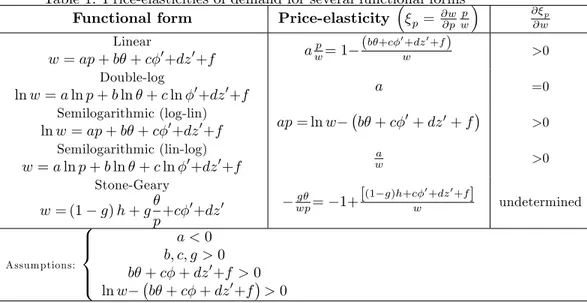
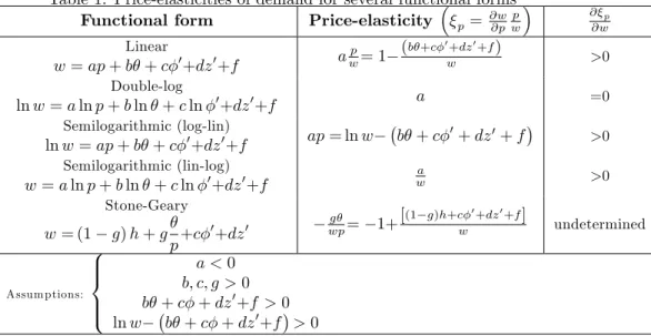
181
Rule, which states that the mark-up of prices over marginal cost will be inversely
182
related to the demand elasticity, so that consumer groups with lower demand
183
elasticities will pay higher prices and vice-versa. The only new term is 1+ ;
184
which re‡ects the scarcity cost. It adds to the price faced by the consumer the
185
opportunity cost of using a scarce resource, but it does not a¤ect the shape of the
186
price schedule. Nonlinear prices may arise in this model because of heterogeneity
187
in the consumers’ preferences (di¤erent price-elasticities), but not because of
188
scarcity. Nonlinear prices would be increasing if the price-elasticities decrease
189
(in absolute value, getting closer to zero) with higher optimal consumption
190
choices and decreasing otherwise.
It should be noted that if the scarcity cost is recovered by a tax which the
192
supplier collects but does not keep, along the lines of what is already done
193
in some European countries, the model will have to be changed accordingly.
194
In particular, if water sources are shared the tax can be de…ned by a Water
195
Authority that oversees several suppliers, since none of them individually will
196
provide adequately for common property (external) scarcity costs. In Portugal
197
a new Water Resource Charge (payed by consumers) was introduced in 2008.
198
The resulting revenue is handed to the River Basin Authorities, the National
199
Water Authorities and a national Tari¤ Balancing Fund.
200
3
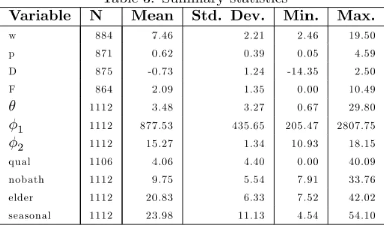
Scarcity with a distribution of consumer types
201
In this section a more complete model is presented, explicitly characterizing
202
demand behavior through the de…nition of a continuum of consumer types.
203
Model development is based on Brown and Sibley (1986) as well as Elnaboulsi
204
(2001). A new parameter, ; is introduced to re‡ect di¤erences in consumer
205
tastes, which can encompass a number of variables. For practical purposes, in
206
the empirical estimation of Section 5 will represent only income, but in theory,
207
customer heterogeneity could stem from any variable which a¤ects residential
208
water demand di¤erently across consumers, such as family size or housing type.
209
A consumer with tastes given by will now enjoy net bene…ts of B(w; ) P (w),
210
where P (w) is the total payment for water consumption. It is assumed that
211
B(0; ) = 0 and that high values of imply higher consumption bene…ts (@B @ >
212
0; @ @w@2B > 0). The distribution of throughout the consumer population is
213
described by a distribution function G( ) and the associated density function
214
g( ): Maximum and minimum values for the taste parameter are represented by
215
and ; respectively, so that G( ) = 1 and G( ) = 0:
216
The …rst order condition of each consumer’s net bene…t maximization is
217
@B(w; )
@w =
dP
dw pm (9)
which is similar to condition (5) except the right-hand side represents the slope
218
of the total payment function, i.e. the marginal price pm: The only restriction to
219
the shape of P (w) is that, if concave, it must be less so than the bene…t function
to ensure that the decision is indeed a maximizing one. Using the consumer’s
221
choice, w( ); the value function is
222
V ( ) = B(w( ); ) P (w( )) (10)
To …nd the properties of the optimal payment function with a scarcity
restric-223
tion, or rather the second best function given the break-even constraint, the
224
following problem can be solved
225 M ax w( ) R V ( )g( )d +R[P (w( )) C(w( ))] g( )d s:t: R [P (w( )) C(w( ))] g( )d = 0 R w( )g( )d W (11)
where the …rst component of the objective function represents consumer surplus
226
aggregating all consumer types, and the second component is pro…t. Some
ma-227
nipulations yield a more tractable version of the problem. Substituting P (w ( ))
228
using equation (10), noting that G( ) 1 =R g( )d and using the envelope
the-229
orem to see that @V
@ =
@B
@ ; consumer surplus can be rewritten using integration
230 by parts 231 Z V ( )g( )d = V ( ) + Z @B @ (1 G( ))d (12)
and the Lagrangian that must be maximized is
L = V ( ) + Z (1 + ) (B (w ( ) ; ) C(w( )) g( ) @B @ (1 G( ))d + 0 B @W Z w( )g( )d 1 C A (13)
For the case where V ( ) = 0; which is the most relevant, the consumer with the lowest taste parameter value has no net bene…t and the …rst order condition
for each is @L @w( ) = 0 (14) = (1 + ) @B @w @C @w g( ) @2B @w@ (1 G( )) g( ) = 0
Using equation (9), a mark-up condition similar to the one from the previous
232
model (equation (8)) can be derived:
233 pm @C@w+1+ pm = 1 + 1 (w; ) (15)
where (w; ) represents the absolute value of the elasticity in each incremental
234
market or consumer group (see Appendix A). As expected, the same
conclu-235
sions as in the discrete case apply to this model regarding the role of customer
236
heterogeneity (here represented by di¤erent ) in generating nonlinear prices,
237
while the scarcity cost does not a¤ect the price schedule shape, but only its
238
level.
239
4
Scarcity in demand, cost, and availability
240
The previous sections have shown that scarcity, represented as a quantity
con-241
straint, has a direct e¤ect that can be seen as an increase in real marginal cost,
242
so that even when coupled with a budget balancing restriction it cannot in itself
243
explain a preference for increasing rates. In order to evaluate other e¤ects of
244
scarcity in a more general sense, this section introduces into the previous models
245
exogenous weather factors, , which a¤ect water availability as well as consumer
246
bene…ts and supply costs. It is assumed that a higher value of means hotter
247
and drier weather, implying that @Bj
@ > 0; @2B
j
@wj@ > 0 (water demand increases, 248
for example due to irrigation or swimming pools), @C@ > 0; @w@@2C > 0 (supply
249
costs are higher due to extra pumping or treatment costs), and dWd < 0 (less
250
available water).
251
Introducing these factors into the models from sections 2 and 3 does not
252
change the fundamental result for the second-best price schedule, expressed by
253
the inverse elasticity rule. The …rst-order conditions for the discrete and the
continuous cases are very similar so we only present results once in a general
255
form, and that is:
256 pm @C(w ; )@w +1+ pm = 1 + 1 (w ; ; ) (16)
Nonlinear pricing is still a consequence of consumer heterogeneity and not
257
of scarcity considerations. However, the shape of the resulting price schedule
258
may now be a¤ected by the in‡uence of the exogenous weather factor on the
259
price elasticities for the di¤erent consumer types.
260
As noted earlier, the marginal unit price and the mark-up for each consumer
261
type or market increment depend inversely on its price-elasticity of demand.
262
Nonlinear prices would be increasing if demand becomes less price-elastic with
263
higher optimal consumption choices and decreasing otherwise. We can
inves-264
tigate the conditions under which the resulting price schedule is increasing,
265
constant or decreasing and how they are a¤ected by the weather parameter.
266
The partial derivative of elasticity with respect to the optimal level of water
267 consumption is: 268 @ (w ; ; ) @w = h @2B(w ; ; ) @w2 i2 w @B(w ; ; )@w hd3B(w ; ; )dw3 w + @2B(w ; ; ) @w2 i h d2B(w ; ; ) dw 2 w i2 (17) The price schedule will be increasing, constant or decreasing according to
269
whether @
@w is negative, null or positive. In order for elasticity to stay the same
270
regardless of consumption, implying that the e¢ cient unit price is constant, the
271
following condition is necessary and su¢ cient:
272 @ (w ; pm) @w = 0 , @B @w h @3B @w 3w + @ 2B @w 2 i @2B @w 2 2 w = 1 (18) Likewise, for @
@w < 0 the expression on the right-hand side of equation (18)
273
must be smaller than 1 and for @
@w > 0 it must be greater than 1. It can be
274
seen that the sign of @ 3B
@w 3, which re‡ects the curvature of the demand
func-275
tion, plays a very important role in determining the shape of the resulting price
schedule. In particular, given an increasing and concave bene…t B(w); @ 3B
@w 3 0
277
is a su¢ cient condition for IBT to be e¢ cient. This condition means the
de-278
mand (marginal bene…t) function is concave, which is related to an accelerating
279
decrease in the marginal bene…t as consumption grows larger.
280
Additionally, we can analyze the impact of the weather parameter on the price schedule by di¤erentiating expression (18) in relation to . We omit the lengthy resulting expression and present only su¢ cient conditions for the result to be negative, i.e., for the in‡uence of the weather variable on the price schedule to reinforce the case for IBT.
@3B @w 3 0 (19) @3B @w 2@ 0 (20) @4B @w 3@ 0 (21)
Condition (19) requires concavity of the demand function, so that IBT would
281
be e¢ cient in the …rst place. Condition (20) implies that the demand function’s
282
negative slope would have to be constant or to become less steep as temperature
283
and dryness increase. Finally, condition (21) requires the demand function’s
cur-284
vature to be constant or to become more concave as temperature and dryness
285
increase. Why do these conditions favour the adoption of IBT in hotter and drier
286
regions or time periods? They seem to create a framework where willingness
287
to pay for water consumption increases more with temperature in high-demand
288
consumers than in those with low-demand pro…les, decreasing the di¤erence in
289
marginal valuation of the initial consumptions and the more extravagant ones.
290
This is consistent with the fact that low-demand residential consumers have
291
a mainly indoor water use which does not vary much with weather conditions,
292
whereas high-demand residential consumers include those with gardens to
sprin-293
kle or swimming pools to …ll in the summer, therefore showing a demand pattern
294
that varies more with weather.
295
High-demand residential consumers are also usually associated with higher
296
income levels (re‡ected in in our model) which means that water expenses can
297
weigh very little on their budget. In this context, relative water demand
ity between high and low-demand users may increase, with
high-income/high-299
demand users being more willing and able to a¤ord the ever scarcer water as
300
temperature increases. The fact that high-income residential consumers tend to
301
have more rigid water demands has been empirically demonstrated for example
302
by Agthe and Billings (1987), Renwick and Archibald (1998) and Mylopoulos,
303
Mentes and Theodossio (2004). In the presence of a Ramsey pricing policy (with
304
price levels inversely related with price-elasticities of demand) this would mean
305
that the tari¤ schedule would tend towards IBT as temperature increases and a
306
bigger share of the water utility’s revenues would be generated by high-demand
307
consumers, which may be an explanation for the fact that IBT are more frequent
308
in countries with hotter and drier climate.
309
Roseta-Palma and Monteiro (2008) provide some additional results for the
310
model. In particular, when marginal cost pricing is followed, if the marginal
311
bene…t functions and the way they respond to weather conditions (@2Bj
@wj@ ) di¤er 312
enough among consumer types, it may be e¢ cient for some consumers (those
313
whose willingness to pay increases more with temperature increases and the
re-314
sulting scarcity) to increase their water consumption in drier periods, while those
315
whose marginal bene…ts change less will save more water. This is not the case
316
in the context of a Ramsey pricing policy, where the greater willingness to pay
317
from such consumer types will be re‡ected in less elastic water demand, so that
318
the water utility will assign them a higher price and they will also consume less
319
water. It can also be shown that the scarcity cost will not necessarily increase
320
with due to the e¤ect on supply costs. The intuitive result that drier and
321
hotter weather will increase scarcity cost arises if the marginal bene…t of water
322
consumption increases more with drier weather conditions than the marginal
323
cost of water supply. This is con…rmed by a dynamic model of water supply
324
enhancement, where the same condition is necessary for optimal investments in
325
water supply to increase with an expected permanent increase in (such as the
326
one that would occur for Mediterranean areas in the context of global warming
327
context).
5
Estimation of Portuguese residential water
de-329
mand
330
In the previous section we included climate variables in a pricing model and
331
analysed the impact of such variables on the price structure. From the
inverse-332
elasticity rule (16) we know that a necessary and su¢ cient condition for
non-333
linear increasing tari¤s is for demand to become less price-elastic with higher
334
levels of water consumption. Therefore, we now estimate water demand and
335
check whether this condition holds, implying that nonlinear increasing tari¤s
336
would be justi…ed.
337
5.1
The importance of the choice of functional form
338
The water demand function can be written as:
339
w = w (p; ; ; z) (22)
where w is the quantity of water demanded and p is the water price. As was
340
previously mentioned, stands for income and represents weather variables
341
such as temperature and precipitation. The vector z can include other household
342
attributes related to water consumption like garden or household size, age and
343
education of household members or the number of water-using appliances, just
344
to name a few. w (: : :) is a parametric function which can take one of several
345
available functional forms.
346
The choice of the functional form for the equation to be estimated is one
347
of the important decisions to be taken by the empirical analyst. Five types
348
of functional forms are more commonly used in the estimation of residential
349
water demand: linear, double-log; semilogarithmic (lin-log or log-lin) and
Stone-350
Geary. The choice of one of these options is not neutral and can have an impact
351
on the results. For instance, Espey, Espey and Shaw (1997) and Dalhuisen,
352
Florax, de Groot and Nijkamp (2003) include a dummy variable for loglinear
353
speci…cations in their meta-analysis of the price-elasticities of water demand
354
estimated in the literature and …nd positive coe¢ cients, meaning that, ceteris
355
paribus, a loglinear speci…cation may result in a less elastic estimate. This
356
fact is known to empirical researchers, despite the fact that it has received less
attention than other aspects of the estimation process, like the choice of the
358
estimation technique (Renzetti (2002)).
359
To see whether demand becomes less price-elastic with higher levels of water
360
consumption we can look directly at the implications of each functional form on
361
the behavior of the price-elasticity of demand. Note that equations (20) and (21)
362
are zero for these functional forms. Table 1 presents the price elasticities for the
363
aforementioned functional forms, where w; p; ; and z are de…ned above and
364
a; b; c; d; f; g; h are parameters. In the Stone-Geary speci…cation, g stands for
365
the …xed proportion of the supernumerary income spent on water (the residual
366
income after the essential needs of water and other goods have been satis…ed)
367
and h stands for the …xed component of water consumption (unresponsive to
368
prices). See Martínez-Espiñeira and Nauges (2004) for more details on the
369
Stone-Geary functional form. The signs for the parameters given in the table are
370
those we expect from the theoretical model. Weather variables with a negative
371
impact on water consumption can be included in vector with a minus sign or
372
with an inverse transformation so that c > 0.
373
We can see that demand becomes less elastic (price elasticity becomes less
374
negative) with higher consumption for most functional forms. Only the
double-375
log case is associated with constant elasticity (this is, in fact, one of the reasons
376
it is so appealing), whereas the Stone-Geary speci…cation has an undetermined
377
result, dependent on the actual values taken by the variables and the associated
378
parameters. Therefore, under the assumptions of our model, IBT will be a
379
natural consequence of demand characteristics for all cases except these two.
380
Insert Table 1 here
381
5.2
The model and the data
382
Annual data on water consumption and water and wastewater tari¤s was
pro-383
vided by the Portuguese National Water Institute (INAG) for the years 1998,
384
2000, 2002 and 2005 (annual consumption was divided by 12 to get average
385
monthly water consumption). It consists of aggregate data for all 278
munici-386
palities in mainland Portugal, excluding the Azores and Madeira archipelagos
for which no information was available. It has been combined with information
388
on income, weather, water quality and household characteristics respectively
389
from the Ministry of Finance and Public Administration, the National Weather
390
Institute (Instituto de Meteorologia, I.P.), the Regulating Authority for Water
391
and Waste (ERSAR) and the National Statistics Institute (INE). Due to the
392
presence of missing data concerning consumption levels it constitutes an
unbal-393
anced panel for the study period. The missing data problem was minimized
394
through direct collection of additional information on consumption and tari¤s
395
from the water and wastewater utilities of each municipality.
396
The estimated model is:
397
wit= f (pit; Dit; Fit; it; 1it; 2it; qualit; nobathi; elderi; seasonali) + i+ "it
398
i IID 0; 2 ; "it= "it 1+ vit; vit IID 0; 2v (23) The formulation of the error variable as the sum of a municipality e¤ect and
399
an autoregressive component is not assumed from the outset but is instead the
400
result of the preliminary analysis.
401
Tables 2 and 3 show the de…nition of the main variables used and some
402
summary statistics. The inclusion of a "di¤erence variable", de…ned by the
403
di¤erence between the variable part of the water and sewage bill and the value
404
it would have had all the volume been charged at the marginal price, is standard
405
in the literature and is meant to capture the income e¤ect of the block subsidy
406
implied by the IBT structure. The …xed part of the bill is included as well
407
because, in theory, it can also have an income-e¤ect on consumption.
408
Note that residential water tari¤s in Portugal are very diverse. For water
409
supply, almost all utilities charge both …xed and variable rates (97.5%), and in
410
the latter 98.6% use IBT. The average number of blocks is 5, although some
411
utilities de…ne as many as 30. The majority of utilities apply the price of each
412
block to the consumption within that block, although 18% bill consumers for
413
the full volume at the price of the highest block, giving rise to marginal price
414
"peaks" at the blocks’ lower limit. Wastewater services are not universally
415
charged, with a zero price in 21% of utilities. Around one third include …xed
416
and variable charges, and another third have only variable rates. In the absence
of sewage meters, these are typically based on water consumption, although
418
they can also be a proportion of the water supply bill (see Monteiro (2009) for
419
a more detailed description).
420
Insert Tables 2 and 3 here
421
5.3
Methodology and estimation
422
We deal with the known endogeneity problem in the price-related variables p
423
and D by creating instrumental variables from the tari¤ unit prices for speci…c
424
volumes of consumption. We look at unit prices for monthly consumptions of
425
1, 5, 10, 15 and 20 m3, (this procedure is also followed by Reynaud, Renzetti
426
and Villeneuve (2005)), the utility’s calculation procedure (whether each unit
427
is charged at the price of its block or all are charged at the unit price of the
428
last block reached) and the type of water utility (municipality, private
com-429
pany, and others). The instruments for p are dummy variables for the type
430
of utility, the utility’s calculation procedure and the tari¤ prices at 5, 10 and
431
15 m3. The instruments for the di¤erence variable are the utility’s calculation
432
procedure and the tari¤ prices at 1, 10 and 20 m3. The Anderson, Sargan and
433
Di¤erence-in-Sargan tests are performed to check on instrument relevance and
434
validity (the xtivreg2 procedure for Stata (Scha¤er (2007)) is used). Regarding
435
the instruments for p, the Anderson underidenti…cation test rejected the null
436
hypothesis of instruments’irrelevance (test statistic: 16.076, p-value for 2(7):
437
0.024) while the Sargan test of instrument validity did not reject the null of
438
instruments’ validity (test statistic: 6.333, p-value for 2(6): 0.387).
Regard-439
ing the instruments for the di¤erence variable, the Anderson test rejected the
440
instrument’s irrelevance (test statistic: 16.368, p-value for 2(4): 0.003) while
441
the Sargan test of instrument validity did not (test statistic: 1.877, p-value for
442
2(3): 0.598). Di¤erence-in-Sargan tests for each instrument (for either p or
443
D) did not reject the null hypothesis of individual instrument validity for any
444
of them.
445
Heteroskedasticity and autocorrelation are detected in the data. We use a
446
GLS estimator with AR(1) disturbances to account for them. The
Pagan Lagrangian multiplier test con…rms the presence of municipal speci…c
448
e¤ects and the Hausman test does not reject the null hypothesis of independence
449
between the municipal e¤ects and the exogenous regressors (this procedure is
450
also followed by Dalmas and Reynaud (2005)). Therefore, the GLS estimator
451
(random e¤ects) is not only e¢ cient but also consistent, so that we choose to
452
use it.
453
Finally, a price perception test (Nieswiadomy and Molina (1991)) was
per-454
formed and con…rmed that consumers respond to the marginal rather than the
455
average price.The test procedure starts by considering a "price perception
vari-456
able" (P ), where k is the price perception parameter to be estimated, p is the
457
marginal price of water services and ap is the average price:
458
P = p ap
p k
(24) A value of 0 for k would mean that consumers were responding to marginal
459
price, rather than average price, while a value of 1 would have the opposite
460
meaning. We adapt the test to our panel data framework by including the
461
ratio app in an estimation of a double-log functional form for water demand
462
together with the marginal price and all other regressors unrelated to the tari¤s
463
with an error structure similar to the one described above. k can be recovered
464
after the estimation by dividing the coe¢ cients associated with ln app and
465
ln p. Because the endogeneity suspicions apply to the average price as well
466
as the marginal price, we start by instrumenting it also. The instruments for
467
the ap are the …xed component of the tari¤, the tari¤ price at 10 m3 and the
468
utility’s calculation procedure. The Anderson underidenti…cation test rejected
469
the instrument’s irrelevance (test statistic: 348.31, p-value for 2(4): 0.00)
470
while the Sargan test of instrument validity did not (test statistic: 348.31,
p-471
value for 2(3): 0.23). Di¤erence-in-Sargan tests for each instrument did not
472
reject the null hypothesis of individual instrument validity for any of them. The
473
coe¢ cients estimated for ln app and ln p are respectively 0.0208 and -0.1110
474
and the value for k is -0.188. After the model was estimated the following
475
nonlinear hypothesis were tested: k = 0 and k = 1. The test statistics were
476
0.23 for k = 0 (p-value for 2(1): 0.6347) and 9.04 for k = 1 (p-value for 2(1):
0.0026), so that k = 0 is not rejected while k = 1 is, meaning that Portuguese
478
consumers do respond to the marginal price and not to the average price of
479
water.
480
5.4
Results
481
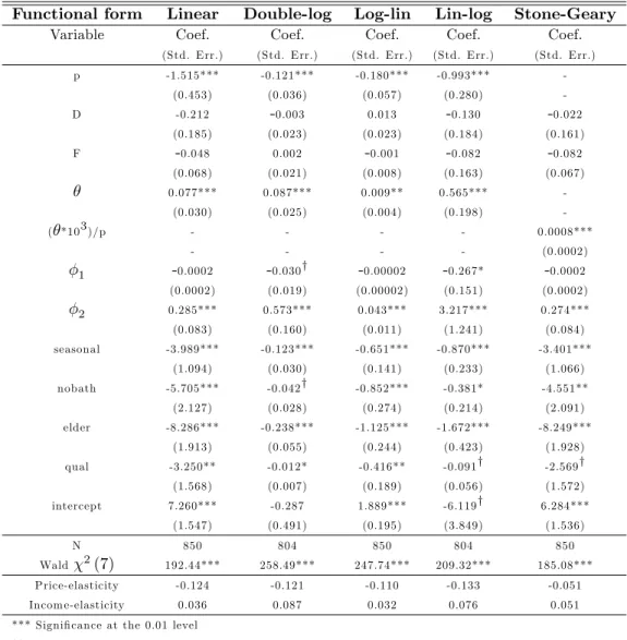
Table 4 presents the estimation results for the functional forms considered in
482
Table 1, including the values derived for price and income elasticities in each
483
case. The fact that the coe¢ cients for the variables which together compose
484
the usual "di¤erence" variable in the Taylor-Nordin price speci…cation are not
485
signi…cantly di¤erent from zero may be a demonstration that consumers are not
486
aware of the block subsidy e¤ect or simply do not react to it since it is small in
487
comparison to their household income.
488
Insert Table 4 here
489
All coe¢ cients have the expected signs and most of them are signi…cant at
490
the 1% level. The value at the sample variable means for the price-elasticity of
491
demand varies between -0.133 and -0.051, a relatively small value, but in line
492
with the established result that water demand is price-inelastic. The estimated
493
values are signi…cantly lower than the value of -0.558 estimated by Martins and
494
Fortunato (2007) for 5 Portuguese municipalities with monthly aggregate data,
495
but is similar to the values estimated by Martínez-Espiñeira and Nauges (2004)
496
and Martínez-Espiñeira (2002) respectively for Seville and Galicia in Spain.
497
The weather-related variables have the expected signs, i.e., water demand
498
increases with temperature and decreases with precipitation, although only
tem-499
perature has a signi…cant coe¢ cient for all functional forms. It would be
inter-500
esting to consider more general functional forms by allowing interaction terms
501
between weather-related variables and price. Thus the households’response to
502
price could vary directly with weather conditions. This approach was tried but
503
the interaction terms turned out non-signi…cant and a substantial amount of
504
multicollinearity was introduced in the estimation, which is probably the
con-505
sequence of using aggregate data. Further tests, using household data, would
506
be needed to allow more general conclusions. Nevertheless, table 1 shows that
with some functional forms, the price-elasticity of demand does depend on the
508
values of these variables.
509
As expected, the percentage of seasonally inhabited dwellings has a
signif-510
icant negative e¤ect on water consumption, as does the percentage of houses
511
without a bathtub or a shower. The negative coe¢ cient for the percentage of
512
people 65 or older also con…rms previous …ndings by Nauges and Thomas (2000),
513
Nauges and Reynaud (2001), Martínez-Espiñeira (2002), Martínez-Espiñeira
514
(2003) and Martins and Fortunato (2007), who have all convincingly shown that
515
older people use less water. Finally the negative (and signi…cant for some
func-516
tional forms) coe¢ cient for qual supports the view that consumers are aware
517
of tap-water quality and do decrease their consumption when they consider it
518
inadequate, perhaps turning to bottled water, private boreholes and wells or
519
public fountains for their drinking and cooking water needs. This …nding adds
520
to the evidence in Ford and Ziegler (1981), the only other study we are aware of
521
which included delivered water quality as an explanatory factor for residential
522
water demand.
523
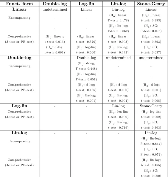
To choose between the functional forms presented in Table 3 we now focus
524
on three di¤erent methods: an encompassing approach (Mizon and Richard
525
(1986)), a comprehensive approach - the J test (Davidson and MacKinnon
526
(1981)), and the PE test (MacKinnon, White and Davidson (1983)). The …rst
527
two approaches are used to compare nonnested models with the same
depen-528
dent variable, while the PE test is used to compare models where consumption
529
is de…ned in natural logarithms with models where it is introduced without that
530
transformation (Greene (2003)). The encompassing approach assumes one of
531
the models being compared as the base model. Then it proceeds to create and
532
estimate a model where the variables from the alternative model not included
533
in the base model are added to it. The null hypothesis of the test is that the
534
coe¢ cients of these additional variables are all zero. A t-test or a Waldman
F-535
test, depending on whether one or more additional regressors were added to the
536
base model, is performed to test the null hypothesis and the validity of the base
537
model. The role of each model can be reversed and the test performed again to
538
the test the validity of the alternative model. The comprehensive approach or
J-test consists of adding to the base model the …tted values of the alternative
540
model and testing whether or not they are signi…cantly di¤erent from zero by
541
means of a t-test. The null hypothesis of a zero coe¢ cient corresponds to a
542
valid base model. Finally, the PE test for the validity of the model with the
543
linear speci…cation of the dependent variable (base model) involves adding to
544
this base model the di¤erence between the natural logarithm of the …tted values
545
for the base model and the …tted values for the alternative model (the one with
546
the dependent variable in logarithms). The null hypothesis that the coe¢ cient
547
of this additional regressor is zero, supports the linear model if it is not rejected
548
and invalidates it against the alternative otherwise. To test the validity of the
549
model with the dependent variable in logarithms we must add to the loglinear
550
model the di¤erence between …tted values of the linear model and the
exponen-551
tial function of the …tted values of the loglinear model. The null hypothesis for
552
this second model states that the coe¢ cient of this additional regressor is zero.
553
If rejected it invalidates the loglinear model, but if not rejected, then it may be
554
preferable. The PE test is an adaptation of the J-test for di¤erent dependent
555
variables.
556
Insert Table 5 here
557
Summing up the results, the Davidson-MacKinnon PE test fails to decide
558
between a semilogarithmic functional form (lin-log) and a double-log functional
559
form. All other speci…cations (Stone-Geary form, linear or the log-lin
semiloga-560
rithmic form) are rejected against at least one of the two previous alternatives.
561
Recall that while a lin-log speci…cation would lead to a recommendation of IBT,
562
the double-log functional form favours a uniform volumetric rate (either of them
563
coupled with a …xed charge, leading to a multi-part tari¤ for the former and a
564
two-part tari¤ for the latter). Hence, our analysis of the Portuguese residential
565
water demand does not enable us to conclude if the IBT typically applied by
wa-566
ter utilities for residential water supply, and to a lesser extent to the wastewater
567
component of the water bill, can be grounded on e¢ ciency reasons.
6
Conclusion
569
We set out to write this paper because of a puzzling question: if increasing block
570
tari¤s for water are not recommended in theoretical economic models, why are
571
they so popular in practice? Clearly, having one block where water is charged
572
at a low price (or even a small free allocation) can be justi…ed by the need to
573
ensure universal access to such a vital good. Yet the IBT schemes we found were
574
much more complex than that. Water managers often mention that increasing
575
rates signal scarcity and as such are a useful tool in reducing resource use. Yet
576
after scanning the literature and developing our own models, a relatively strong
577
conclusion stands out: the best way to allocate water when scarcity occurs is
578
to raise its price in accordance with its true marginal cost, which includes the
579
scarcity cost. Nonlinear pricing is a consequence of consumer heterogeneity and
580
not speci…cally of scarcity considerations.
581
However, we do show that the shape of the resulting price schedule may,
582
in certain circumstances, be a¤ected by the in‡uence of the exogenous weather
583
factor on the price-elasticities of the demands for the di¤erent consumer types.
584
If high demand consumers’ willingness to pay for water rises more with
tem-585
perature increases relative to low demand consumers then IBT may be more
586
appropriate in countries with hotter and drier climates. This is consistent with
587
the fact that Mediterranean European countries are often mentioned in OECD
588
reports to make extensive use of IBT.
589
In a context where volumetric rates are the only available instrument for
590
variable-cost recovery, we tested the condition for IBT to be e¢ cient, derived
591
from our model, through the estimation of Portuguese residential water demand
592
and showed that the choice of functional form is crucial. After the appropriate
593
speci…cation tests, we are left with an inconclusive choice between a
semiloga-594
rithmic lin-log functional form and a double-log speci…cation: the former favours
595
IBT, while the latter favours two-part tari¤s. Thus we have not been able to
596
prove that the use of IBT can be grounded in e¢ ciency, but such a possibility
597
could not be dismissed either. Therefore, it is possible that the widespread use
598
of IBT in Portugal is actually e¢ cient, although decision makers may see it
599
mainly as an issue of equity or perceived water conservation e¤ects. Moreover,
given that results depend on the speci…c demand function, additional research
601
with non-parametric (or semi-parametric) techniques should be carried out.
602
Our demand estimation also produced some results that are relevant in
them-603
selves. Besides the usual positive impact of income, temperature and
water-604
using appliances and the negative impact of price and the proportion of elderly
605
people, we also show that the proportion of seasonally inhabited dwellings and
606
reduced water quality on delivery can have a signi…cant negative in‡uence on
607
the amount of water households consume.
608
Further research should focus on gathering household-level data to increase
609
data variability and improve the choice of the functional form. A database with
610
enough detail would allow the use of discrete-continuous choice models and to
611
estimate the unconditional (on the block choice) price-elasticity of demand. If
612
intra-annual data is available, seasonal e¤ects of weather variables and seasonal
613
house occupancy on water demand could be ascertained. Finally, the current
614
demand analysis could be combined with water supply information, taking into
615
consideration the reduction in water availability which is expected for Portugal,
616
due to climate change. Such work is relevant for an assessment of climate change
617
impacts in the residential water sector.
618
7
Acknowledgements
619
This paper was created within the research project POCI
2010/EGE/61306/2004-620
Tarifaqua, supported by the FCT - POCI 2010, co-…nanced by the European
621
fund ERDF. We are indebted to the institutions which diligently provided the
622
data, namely the INSAAR team at the Portuguese National Water Institute
623
(INAG). The authors thank José Passos, Ronald Gri¢ n, Steven Renzetti, and
624
three anonymous referees for valuable comments. Any errors and omissions are
625
the authors’own responsibility.
626
A
Appendix - Derivation of equation 15
627
This Appendix contains the derivation of equation (15). See also Brown and
628
Sibley (1986, pp.205-6).
(1 + ) @B@w @C@w g( ) @w@@2B(1 G( )) g( ) = 0 630 since @B(w; ; )@w =dP dw pm 631 , (1 + ) pm @C@w g( ) g( ) = @ 2B @w@ (1 G( )) , 632 , pm @C@w+1+ pm =1+ 1 pm @2B @w@ (1 G( )) g( ) , 633 , pm @C@w+1+ pm =1+ p1 m 1 @ @pm (1 G( )) g( ) , 634
where indicates the marginal consumer group ( = (Q; P (Q)))
635
De…ning marginal willingness to pay, (w; ), the self-selection condition is
636 (w; ) = pm;so that d dpm = 1 , @ @ @ @pm = 1 , @ @pm = 1 , @ @pm = 1 > 0 637 Since Bw @2B (w; ) @w@ @ (w; ) @ , @ @pm = 1 B w 638 Finally, 639 , pm @C@w+1+ pm =1+ 1 pm @ @pm g ( ) (1 G( )) , 640 , pm @C@w+1+ pm =1+ 1 (w; pm) 641
which is the condition in the text. (w; pm) emerges through the following
642 manipulations: 643 @ ln pm(w) @pm(w) = 1 pm(w) 644 d ln [1 G ( )] dpm(w) = @ ln [1 G ( )] @ ln pm(w) @ ln pm(w) @pm(w) , 645 , [1 1G ( )] g ( ) @ @pm = @ ln [1 G ( )] @ ln pm(w) 1 pm(w) , 646 , d ln [1d ln p G ( )] m(w) = g ( ) @ @pm pm(w) [1 G ( )] , @ ln [1 G ( )] @ ln pm(w) = g ( ) @ @pm pm(w) [1 G ( )] ] 647
[note that in general: xf (x) = @f (x) @x x f (x)= @ ln f (x) @ ln x ] 648
References
649
Agthe, D. E. and Billings, R. B. (1987), ‘Equity, price elasticity and
house-650
hold income under increasing block rates for water’, American Journal of
651
Economics and Sociology 46(3), 273–286.
652
APA/MAOTDR (2008), REA 2007 Portugal - Relatório de Estado Do
Am-653
biente 2007, Agência Portuguesa do Ambiente, Ministério do Ambiente,
654
do Ordenamento do Território e do Desenvolvimento Regional, Amadora,
655
Portugal.
656
Boland, J. J. and Whittington, D. (2000), The political economy of water tari¤
657
design in developing countries: Increasing block tari¤s versus uniform price
658
with rebate, in A. Dinar, ed., ‘The Political Economy of Water Pricing
659
Reforms’, Oxford University Press, New York, USA, chapter 10, pp. 215–
660
235.
661
Brown, S. and Sibley, D. (1986), The Theory of Public Utility Pricing,
Cam-662
bridge University Press, Cambridge, UK.
663
Dalhuisen, J. M., Florax, R. J. G. M., de Groot, H. L. F. and Nijkamp, P.
664
(2003), ‘Price and income elasticities of residential water demand: A
meta-665
analysis’, Land Economics 79(2), 292–308.
666
Dalmas, L. and Reynaud, A. (2005), Residential water demand in the
slo-667
vak republic, in P. Koundouri, ed., ‘Econometrics Informing Natural
Re-668
sources Management: Selected Empirical Analyses’, Edward Elgar
Pub-669
lishing, Cheltenham, UK, chapter 4, pp. 83–109.
670
Davidson, R. and MacKinnon, J. G. (1981), ‘Several tests for model speci…cation
671
in the presence of alternative hypothesis’, Econometrica 49(3), 781–793.
672
EC (2007), Addressing the challenge of water scarcity and droughts in the
673
european union, Communication from the Commission to the European
674
Parliament and the Council COM(2007) 414 …nal, European Commission,
675
Brussels, Belgium.
EEA (2009), Water resources across europe - confronting water scarcity and
677
drought, EEA Report 2/2009, European Environment Agency,
Copen-678
hagen, Denmark.
679
Elnaboulsi, J. C. (2001), ‘Nonlinear pricing and capacity planning for water and
680
wastewater services’, Water Resources Management 15(1), 55–69.
681
Elnaboulsi, J. C. (2009), ‘An incentive water pricing policy for sustainable water
682
use’, Environmental and Resource Economics 42(4), 451–469.
683
Espey, M., Espey, J. and Shaw, W. D. (1997), ‘Price elasticity of residential
de-684
mand for water: A meta-analysis’, Water Resources Research 33(6), 1369–
685
1374.
686
EU (2000), ‘Directive 2000/60/EC of the european parliament and of the council
687
establishing a framework for the community action in the …eld of water
688
policy - EU water framework directive’, O¢ cial Journal (OJ L 327).
689
Ford, R. K. and Ziegler, J. A. (1981), ‘Intrastate di¤erences in residential water
690
demand’, The Annals of Regional Science 15(3), 20–30.
691
Greene, W. H. (2003), Econometric Analysis, 5th edn, Prentice-Hall, New
Jer-692
sey, USA.
693
Gri¢ n, R. C. (2001), ‘E¤ective water pricing’, Journal of the American Water
694
Resources Association 37(5), 1335–1347.
695
Gri¢ n, R. C. (2006), Water Resource Economics: The Analysis of Scarcity,
696
Policies, and Projects, MIT Press, Cambridge, Massachusetts, USA.
697
Hanemann, W. M. (1997), Price and rate structures, in D. D. Baumann, J. J.
698
Boland and W. M. Hanemann, eds, ‘Urban Water Demand Management
699
and Planning’, McGraw-Hill, New York, USA, pp. 137–179. Chap. 5.
700
Hewitt, J. A. (2000), An investigation into the reasons why water utilities choose
701
particular residential rate structures, in A. Dinar, ed., ‘The Political
Econ-702
omy of Water Pricing Reforms’, Oxford University Press, New York, USA,
703
chapter 12, pp. 259–277.
INAG/MAOTDR (2008), Relatório do estado do abastecimento de água e de
705
saneamento de águas residuais - campanha INSAAR 2006, Technical
re-706
port, Instituto da Água, Ministério do Ambiente, do Ordenamento do
Ter-707
ritório e do Desenvolvimento Regional, Lisboa, Portugal.
708
Komives, K., Foster, V., Halpern, J. and Wodon, Q. (2005), Water, Electricity,
709
and the Poor: Who Bene…ts from Utility Subsidies?, World Bank,
Wash-710
ington D.C.
711
Krause, K., Chermak, J. M. and Brookshire, D. S. (2003), ‘The demand for
712
water: Consumer response to scarcity’, Journal of Regulatory Economics
713
23(2), 167–191.
714
MacKinnon, J. G., White, H. and Davidson, R. (1983), ‘Tests for model
spec-715
i…cation in the presence of alternative hypothesis: Some further results’,
716
Journal of Econometrics 21(1), 53–70.
717
Martínez-Espiñeira, R. (2002), ‘Residential water demand in the northwest of
718
spain’, Environmental and Resource Economics 21(2), 161–187.
719
Martínez-Espiñeira, R. (2003), ‘Estimating water demand under
increasing-720
block tari¤s using aggregate data and proportions of users per block’,
En-721
vironmental and Resource Economics 26(1), 5–23.
722
Martínez-Espiñeira, R. and Nauges, C. (2004), ‘Is all domestic water
consump-723
tion sensitive to price control?’, Applied Economics 36(15), 1697–1703.
724
Martins, R. and Fortunato, A. (2007), ‘Residential water demand under block
725
rates - a portuguese case study’, Water Policy 9(2), 217–230.
726
Mizon, G. E. and Richard, J. F. (1986), ‘The encompassing principle and its
727
application to testing non-nested hypothesis’, Econometrica 54(3), 654–
728
678.
729
Moncur, J. E. T. and Pollock, R. L. (1988), ‘Scarcity rents for water: A valuation
730
and pricing model’, Land Economics 64(1), 62–72.
Monteiro, H. (2005), Water pricing models: A survey, Working Paper 2005/45,
732
DINÂMIA, Research Centre on Socioeconomic Change, Lisboa, Portugal.
733
Monteiro, H. (2009), Water Tari¤s: Methods for an E¢ cient Cost Recovery
734
and for the Implementation of the Water Framework Directive in
Portu-735
gal, Phd thesis, Technical University of Lisbon, School of Economics and
736
Management, Lisboa, Portugal.
737
Mylopoulos, Y. A., Mentes, A. K. and Theodossio, I. (2004), ‘Modeling
res-738
idential water demand using household data: A cubic approach’, Water
739
International 29(1), 105–113.
740
Nauges, C. and Reynaud, A. (2001), ‘Estimation de la demande domestique
741
d’eau potable en france’, Revue Economique 52(1), 167–185.
742
Nauges, C. and Thomas, A. (2000), ‘Privately-operated water utilities,
munic-743
ipal price negotiation, and estimation of residential water demand: The
744
case of france’, Land Economics 76(1), 68–85.
745
Nieswiadomy, M. L. and Molina, D. J. (1991), ‘A note on price perception in
746
water demand models’, Land Economics 67(3), 352–359.
747
OECD (2003), Social Issues in the Provision and Pricing of Water Services,
748
OECD - Organisation for Economic Co-operation and Development, Paris,
749
France.
750
OECD (2006), Water: The Experience in OECD Countries, Environmental
751
Performance Reviews, OECD - Organisation for Economic Cooperation
752
and Development, Paris, France.
753
OECD (2009), Managing Water for All: An OECD Perspective on Pricing and
754
Financing, OECD Publishing, Paris, France.
755
Renwick, M. E. and Archibald, S. O. (1998), ‘Demand side management
poli-756
cies for residential water use: Who bears the conservation burden?’, Land
757
Economics 74(3), 343–359.
Renzetti, S. (2002), The Economics of Water Demands, Kluwer Academic
Pub-759
lishers, Boston, USA.
760
Reynaud, A., Renzetti, S. and Villeneuve, M. (2005), ‘Residential water demand
761
with endogenous pricing: The canadian case’, Water Resources Research
762
41(11), W11409.1–W11409.11.
763
Roseta-Palma, C. and Monteiro, H. (2008), Pricing for scarcity, Working Paper
764
2008/65, DINÂMIA, Research Centre on Socioeconomic Change, Lisboa,
765
Portugal.
766
Scha¤er, M. E. (2007), ‘Xtivreg2: Stata module to perform extended IV/2SLS,
767
GMM and AC/HAC, LIML and k-class regression for panel data models’,
768
http://ideas.repec.org/c/boc/bocode/s456501.html.
769
Wilson, R. (1993), Nonlinear Pricing, Oxford University Press, New York, USA.
770
Table 1: Price-elasticities of demand for several functional forms
Functional form Price-elasticity p= @w
@p p w @ p @w Linear w = ap + b + c 0+dz0+f a p w= 1 (b +c 0+dz0+f) w >0 Double-log ln w = a ln p + b ln + c ln 0+dz0+f a =0 Semilogarithmic (log-lin) ln w = ap + b + c 0+dz0+f ap = ln w b + c 0+ dz0+ f >0 Semilogarithmic (lin-log) w = a ln p + b ln + c ln 0+dz0+f a w >0 Stone-Geary w = (1 g) h + g p+c 0+dz0 wpg = 1+ [(1 g)h+c 0+dz0+f] w undetermined A ssum ptions: 8 > > < > > : a < 0 b; c; g > 0 b + c + dz0+f > 0 ln w b + c + dz0+f > 0
Table 2: De…nition of variables
Variable De…nition
w A verage m onthly water consum ption (m3/m onth)
p M arginal price of water supply and sewage disp osal (e/m3)
D D i¤erence variable / variable part of the water and sewage bill - (M P*Water) (e/m onth) F Fixed part of the water and sewage bill (e/m onth)
Per capita available incom e (e103/p erson/year) 1 Total annual precipitation (m m )
2 A verage annual tem p erature (oC )
qual % of delivered water analysis failing to com ply w ith m andatory param eters nobath % of regularly inhabited dwellings w ithout shower or bathtub
elder % of p opulation w ith 65 or m ore years of age seasonal % of dwellings w ith seasonal use
Table 3: Summary statistics
Variable N Mean Std. Dev. Min. Max.
w 884 7.46 2.21 2.46 19.50 p 871 0.62 0.39 0.05 4.59 D 875 -0.73 1.24 -14.35 2.50 F 864 2.09 1.35 0.00 10.49 1112 3.48 3.27 0.67 29.80 1 1112 877.53 435.65 205.47 2807.75 2 1112 15.27 1.34 10.93 18.15 qual 1106 4.06 4.40 0.00 40.09 nobath 1112 9.75 5.54 7.91 33.76 elder 1112 20.83 6.33 7.52 42.02 seasonal 1112 23.98 11.13 4.54 54.10
Table 4: Estimation results
Functional form Linear Double-log Log-lin Lin-log Stone-Geary
Variable Coef. Coef. Coef. Coef. Coef.
(Std. Err.) (Std. Err.) (Std. Err.) (Std. Err.) (Std. Err.)
p -1.515*** -0.121*** -0.180*** -0.993*** -(0.453) (0.036) (0.057) (0.280) -D -0.212 -0.003 0.013 -0.130 -0.022 (0.185) (0.023) (0.023) (0.184) (0.161) F -0.048 0.002 -0.001 -0.082 -0.082 (0.068) (0.021) (0.008) (0.163) (0.067) 0.077*** 0.087*** 0.009** 0.565*** -(0.030) (0.025) (0.004) (0.198) -( *103)/p - - - - 0.0008*** - - - - (0.0002) 1 -0.0002 -0.030y -0.00002 -0.267* -0.0002 (0.0002) (0.019) (0.00002) (0.151) (0.0002) 2 0.285*** 0.573*** 0.043*** 3.217*** 0.274*** (0.083) (0.160) (0.011) (1.241) (0.084) seasonal -3.989*** -0.123*** -0.651*** -0.870*** -3.401*** (1.094) (0.030) (0.141) (0.233) (1.066) nobath -5.705*** -0.042y -0.852*** -0.381* -4.551** (2.127) (0.028) (0.274) (0.214) (2.091) elder -8.286*** -0.238*** -1.125*** -1.672*** -8.249*** (1.913) (0.055) (0.244) (0.423) (1.928)
qual -3.250** -0.012* -0.416** -0.091y -2.569y
(1.568) (0.007) (0.189) (0.056) (1.572) intercept 7.260*** -0.287 1.889*** -6.119y 6.284*** (1.547) (0.491) (0.195) (3.849) (1.536) N 850 804 850 804 850 Wald 2(7) 192.44*** 258.49*** 247.74*** 209.32*** 185.08*** Price-elasticity -0.124 -0.121 -0.110 -0.133 -0.051 Incom e-elasticity 0.036 0.087 0.032 0.076 0.051
*** Signi…cance at the 0.01 level ** Signi…cance at the 0.05 level * Signi…cance at the 0.10 level y Signi…cance at the 0.15 level