Repositório ISCTE-IUL
Deposited in Repositório ISCTE-IUL:
2019-05-24
Deposited version:
Post-print
Peer-review status of attached file:
Peer-reviewed
Citation for published item:
Leão, E. R. & Leão, P. R. (2007). Modelling the central bank repo rate in a dynamic general equilibrium framework. Economic Modelling . 24 (4), 571-610
Further information on publisher's website:
10.1016/j.econmod.2006.12.003
Publisher's copyright statement:
This is the peer reviewed version of the following article: Leão, E. R. & Leão, P. R. (2007). Modelling the central bank repo rate in a dynamic general equilibrium framework. Economic Modelling . 24 (4), 571-610, which has been published in final form at
https://dx.doi.org/10.1016/j.econmod.2006.12.003. This article may be used for non-commercial purposes in accordance with the Publisher's Terms and Conditions for self-archiving.
Use policy
Creative Commons CC BY 4.0
The full-text may be used and/or reproduced, and given to third parties in any format or medium, without prior permission or charge, for personal research or study, educational, or not-for-profit purposes provided that:
• a full bibliographic reference is made to the original source • a link is made to the metadata record in the Repository • the full-text is not changed in any way
The full-text must not be sold in any format or medium without the formal permission of the copyright holders. Serviços de Informação e Documentação, Instituto Universitário de Lisboa (ISCTE-IUL)
Av. das Forças Armadas, Edifício II, 1649-026 Lisboa Portugal Phone: +(351) 217 903 024 | e-mail: [email protected]
Elsevier Editorial System(tm) for Economic Modelling
Manuscript Draft
Manuscript Number: ECMODE-D-05-00045R2
Title: Modelling the Central Bank Repo Rate in a Dynamic General Equilibrium Framework Article Type: Full Length Article
Keywords: dynamic general equilibrium; central bank repo rate; currency-deposits ratio; required reserve ratio; composition of investment expenditure.
Corresponding Author: Dr. Emanuel Reis Leao, PhD Corresponding Author's Institution: ISCTE
First Author: Emanuel Leao, PhD
Order of Authors: Emanuel Leao, PhD; Pedro Leao, PhD
Abstract: This paper incorporates two components of a modern monetary system into a standard real business cycle model: a central bank which lends reserves to commercial banks and charges a repo interest rate; and banks which make loans under a fractional reserve system and thereby create money.
We examine the response of our model to shocks in the monetary base, in the currency-deposits ratio and in the required reserve ratio. Our main finding is that all these monetary shocks lead to changes in the
Prof.
Emanuel
R.
Leao
Departamento
de
Economia,
Instituto
Superior
de
Ciencias
do Trabalho e da Empresa,
Avenida das Forcas Armadas,
P – 1649-026 Lisboa,
PORTUGAL
Phone: 00351217903236
Fax: 00351217903933
Email:
[email protected]
Lisboa, 12 October 2006
Dear Professor Stephen G. Hall
Dept of Economics
University of Leicester
University Rd
Leicester
LE1 7RH
United Kingdom
Please find attached the following documents:
1. The new revised version of the paper by myself and P. Leao, entitled
“Modelling the Central Bank Repo Rate in a Dynamic General Equilibrium Framework”;
2. A letter containing our reply to the referee's comments.
With best compliments,
(Emanuel Reis Leao)
1
Description of the way we addressed the referee’s comments
(Artic le title: “Modelling the Central Bank Repo Rate in a Dynamic General Equilib rium Framework”)It seems to us that the essence of the referee’s comments can be summarized as follows: “I could not determine if you are simply unclear in explaining the
banking and household sectors”, “the quantity of money and the role of inflation in this model” or “if you are not doing what you set out to do”.
Our reply:
1. “I could not determine if you are simply unclear in explaining the banking and household sectors”.
Here, the referee is surely concerned with the strategy we followed to model the supply of money and with the adequacy of the monetary flows among the banks, households and firms.
In general, there are two possible ways of modelling the supply of money and the monetary flows among the banks, households and firms.
One is to assume, like Christiano and Eichenbaum (1995, p. 1115-6), that “at the beginning of time t the representative household is in possession of the economy’s entire money stock, Mt … The household [then] allocates its cash between two uses: loans to the financial intermediary, Nt, and purchases of the consumption good. In addition to Nt, another source of funds for the financial intermediary is lump sum injections, Xt, of cash by the monetary authority. [Finally], the financial intermediary lends its cash, Nt + Xt, to the firm.”
This strategy has two shortcomings. First, it does not explain how the household obtains the cash in the first place. Second, it does not include a money-multiplier mechanism.
2
We follow an alternative strategy, adopted among others by Godley and Lavoie (2001). This recognizes that, in modern monetary systems, money is originally created when banks provide credit to the non-banking sector (households, firms or the government). This strategy has two advantages. First, it explains how money is originally created in the economy. Second, it involves the creation of deposits and a money-multiplier mechanism.
On page 5 of the new version of the paper, we now expla in in more detail the strategy we followed to model the supply of money.
In the real world, firms borrow to finance investment and/or to pay wages in advance, i.e., before production and sales have taken place. In turn, households borrow in order to purchase goods before they receive their incomes. Examples include loans to finance the purchase of houses and of various durable consumption goods (cars, etc.), and the use of credit cards for daily payments.
We studied both possibilities: household borrowing and firm borrowing. However, in this paper we only presented the model where banks provide credit to the household sector. The reason is that it gives a simpler picture of the monetary flows in the economy. In the paper submitted, the monetary flows are as follows:
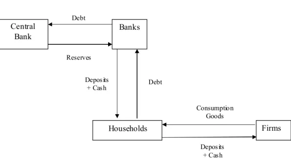
- At the beginning of the period there is no money in the economy. The central bank then lends reserves to banks which use them to support loans to households under a fractional reserve system. Households borrow from the banks in order to buy consumption goods from the firms. During the period, households spend all of their money on consumer goods. Suppose, as an example, that the central bank decides to lend $2 to the banking system and that the reserve-deposits ratio is 2%. In this case – and assuming also that economic agents choose to hold all of their money in the form of deposits - the total amount of credit that banks can supply is $100. Under these
3
assumptions, the economic flows during the period can be described by the following figure:1
- Hence, at the end of the period, the entire money stock of the economy ($100) is held by the firms. Afterwards, firms return this amount to the households in the form of wages and dividends:
1 If we instead consider that economic agents choose to hold part of their money in the form of circulation, the details of the monetary flows become somewhat more complicated, but their basic structure remains the same (see pp. 5-6 and figures A to E of the new version of the paper). Deposits = $100 Households Central Bank Banks Firms Deposits = $ 100 = $ 100 Debt Debt = $2 Consumption Goods = $100 Reserves = $2 Figure A
4
- Suppose additionally that the bank interest rate is 3% and that the central bank repo rate is 1%. Then, the households use part of the money ($3 = 3% of $100) to pay interest on the debt contracted at the beginning of the period – but these $3 are immediately returned to the households. As shown in figure C, they are returned in three ways: (i) banks use part of the interest received from the households to pay interest to the central bank ($0.02 = 1% of $2), which then transfers that amount to the households as a lump-sum transfer; (ii) another portion of the interest received by the banks (say, $1) is used to pay the physical capital that they obtained from the firms, which then pay that amount to the households as wages and dividends; (iii) the remaining part of the interest ($1.98) is paid to the households as bank dividends and wages.
Deposits = $100 Firms Households
5
- Hence, households are again in possession of the $100 that they had initially borrowed. They use them to pay their debt to the banks:
Consequently, households are left with no money.
- In turn, banks no longer have any deposits on the liabilities side of their balance sheets, and so no longer need reserves. The reserves they had obtained at the beginning of the period are therefore returned to the central bank:
Households
Deposits = $100
Figure D
Banks Cancellation of the debt = $100
Households Banks Interest = $3 (=3%.$100) Wages + Dividends = (say) $1 Central Bank Interest = $0.02 (=1%.$2) Lump-sum Transfer = $0.02 Firms
Wages + Dividends = (say) $ 1.98 Physical
capital
Deposits = (say) $1
6
- Hence, banks are left with no reserves. As we have seen, households and firms also end the period without any money. As a result, at the start of the next period there is no money in the economy, and therefore the whole process must be repeated again.
In the new version of the paper, we include a similar explanation of the monetary flows in the economy, but with two differences. First, we present the flows in general terms, without the numerical example. Second, we assume, as our model does, that economic agents choose to hold part of their money in the form of circulation. See pp. 5-6 and figures A to E at the end of the revised paper.
We also considered the case where deposits are originally created when banks provide credit to firms. In this case, firms borrow to pay wages in advance, i.e., before production and sales have taken place. As mentioned in the appendix of the paper, the results we obtained in this setting were not very different from the results quoted in the paper. However, the description of the economic flows is more complicated: at the beginning of a period, there is no money. The central bank then lends reserves to banks, which use them to support loans to firms. These loans create deposits, which firms use to pay wages. In this way, the firms’ deposits become households’ deposits. Households then use the deposits to buy consumption goods from the firms. The deposits are therefore transferred from the households’ bank accounts back to the
Banks
Reserves = $2
Figure E
Central Bank Cancellation of the debt = $2
7
firms’ bank accounts. Then, the firms use the deposits to pay dividends, which are spent in the purchase of the firms’ goods. Therefore, the deposits end up again in the firms’ bank accounts. They use part of the money to pay banks the interest on the debt contracted at the beginning of the period – but it is returned to them (because banks pay wages and dividends to the households who then use the money to buy goods from the firms). Hence, firms again possess the money they initially borrowed, and use it to pay off their bank loans. Consequently, firms are left with no money. As far as the banks are concerned, this means that they no longer have checkable deposits on the liabilities side of their balance sheets, and so no longer need reserves. Therefore, they use their excess reserves to repay their debt to the central bank and are left with no reserves.
2. “As I proceeded through the paper, I became very confused about the quantity of money and the role of inflation in this model”.
As can be seen in equation (14), in each period the quantity of money in our model is determined by the amount of reserves that the central bank decides to lend to the banking sector and by the money multiplier (which depends on the reserve-deposits and currency-reserve-deposits ratios).
In turn, the quantity of money determines the price level. In fact, as mentioned at the beginning of section 9.3, a 1% permanent increase in the money supply leads to a 1% permanent increase in the price level and has no effect whatsoever on the real variables of the model. On the other hand, in the case where the increase in the money supply is seen as temporary, the impact on the real variables is very small.
Finally, we present an explanation of the role of inflation in our model. A temporary increase in the quantity of reserves leads to a proportionate increase in the
8
price level, followed by a gradual decrease back to its steady-state level (Figure 24). This involves a period of negative inflation, which is anticipated by the economic agents. In turn, the emergence of negative expected inflation explains the small impact on the real interest rate (Figure 23), despite the strong fall in nominal interest rates (Figures 25 and 26). As a result, consumption, investment and the other real variables of the model do not undergo significant changes after an increase in central bank liquidity.
In the new version of the paper, section 9.3 now includes these explanations.
Modelling the Central Bank Repo Rate
in a Dynamic General Equilibrium
Framework*
Emanuel R. Leao
Departament of Economics, Instituto
Superior de Ciencias do Trabalho e da
Empresa and Dinamia, Avenida das Forcas
Armadas, 1649-026 Lisboa, Portugal
Phone 00351217903236
Fax 00351217903933
E-mail: [email protected]
Pedro
R.
Leao
Department of Economics, Instituto
Superior de Economia e Gestao, Technical
University of Lisbon, Rua Miguel Lupi, No
20, 1200 Lisboa, Portugal
E-mail: [email protected]
October 2006
*We thank helpful comments by Alan J. Sutherland, Peter N. Smith, Morten O. Ravn and
an anonymous referee. They are not, in any way, responsible for anything written in
this paper.
Modelling the Central Bank Repo Rate
in a Dynamic General Equilibrium Framework
Abstract
This paper incorporates two components of a modern monetary
system into a standard real business cycle model: a central bank
which lends reserves to commercial banks and charges a repo
interest rate; and banks which make loans under a fractional
reserve system and thereby create money.
We examine the response of our model to shocks in the monetary
base, in the currency-deposits ratio and in the required reserve
ratio. Our main finding is that all these monetary shocks lead to
changes in the composition of total investment between the
banking and the non-banking sectors.
Keywords: dynamic general equilibrium; central bank repo rate;
currency-deposits ratio; required reserve ratio; composition of
investment expenditure.
1
Introduction
Modern monetary systems have two important features. First, there is a central bank which lends reserves to commercial banks and charges a repo interest rate (e.g., the “main refinancing rate” of the European Central Bank). Second, there are banks which make loans under a fractional reserve system and thereby create money. This paper is an attempt to incorporate these elements into a standard Real Business Cycle (RBC) model.
RBC models were launched by Kydland and Prescott (1982) and Long and Plosser (1983), and were later given a more consistent framework by Hansen (1985) and King, Plosser and Rebelo (1988). These were dynamic general equilibrium models with a productive sector, intertemporal optimization under rational expectations and perfectly flexible prices - but without money. Later research added new dimensions to the basic model. Cooley and Hansen (1989) first incorporated money into RBC models by using a cash-in-advance constraint to derive the demand for money and assuming that money was supplied through lump-sum transfers from a monetary authority. Fuerst (1992) and Christiano & Eichenbaum (1992, 1995) made further extensions by introducing a banking system which receives cash injections from the central bank and lends money to the economy. However, unlike in the real world, the cash injections received from the monetary authority in their models are costless lump-sum transfers, and banks do not operate under a fractional reserve system.
By contrast, this paper extends the standard RBC model by explicitly including (i) a central bank that lends reserves to banks and charges a repo interest rate; and (ii) banks which make loans under a fractional reserve system and thereby create money. This extended framework will allow us to look at the impact of monetary shocks which have not so far been considered in the RBC literature. In particular, we will study how the economy and the banking system are affected by changes in the repo rate and by changes in the money multiplier (arising from variations in the currency-deposits ratio and/or in the required reserve ratio).
It should be acknowledged that other work has already modelled the central bank repo rate in a dynamic general equilibrium framework. Notable examples are the flexible-price models of Calvo and Vegh (1990, 1995) and Lahiri and Vegh (2003), and the sticky-price models of Clarida,
Gali and Gertler (1999) and McCallum and Nelson (1999). However, unlike the present paper, these models do not include a fractional reserve banking system, nor a productive sector with endogenous capital accumulation. Additionally, the present paper goes beyond the qualitative comparison between the properties of the model and the stylized facts. In the RBC vein, we calibrate our model and then use it to generate artificial data that can be compared with actual data. In this way, the present paper attempts to meet the challenge set forth by Lucas (1980) when he wrote that one of the functions of theoretical economics is to provide fully articulate, artificial economic systems that can serve as laboratories for macroeconomic analysis.1
We start by modelling the typical behaviour of households, firms and banks. The first order conditions of these agents’ decision problems, together with the market clearing conditions, define the competitive equilibrium of the economy. Next, this system is log-linearized around the steady-state values of its variables and then calibrated using Postwar U.S. data. Finally, we examine the response of the model to shocks in the monetary base, in the currency-deposits ratio and in the required reserve ratio. Our main finding is that all these monetary shocks lead to changes in the composition of investment between the banking sector and the non-banking sector. More specifically, an increase in reserves by the central bank which is seen as temporary leads to a strong increase in investment by banks at the expense of investment by non-bank firms. In contrast, an increase in either the currency-deposits ratio or in the required reserve ratio leads to a fall in bank investment in favour of a rise in non-bank investment.
The structure of the article is as follows. In section 2, we characterize the economic envi-ronment: economic flows, preferences, technology, resource constraints and market structure. In section 3, we describe the typical bank’s behaviour and its relation with the central bank. Sec-tions 4 and 5 deal respectively with the typical firm’s behaviour and with the typical household’s behaviour. In section 6, we write down the market clearing conditions. Section 7 presents the system that describes the competitive equilibrium and section 8 reports the calibration of the model. In section 9, we look at the impacts of increases in central bank liquidity, and of changes in the currency-deposits ratio and in the required reserve ratio. Section 10 provides an overview and concludes.
1On this issue, see Rebelo (2005) and King and Rebelo (1999).
2
The Economic Environment
We consider a closed economy with no government. In this economy, there are H homogeneous households, F homogeneous firms, L homogeneous banks and one central bank. Firms and banks are owned by households. As a consequence, both firms’ and banks’ profits are distributed to households (the shareholders) at the end of each period. There is only one physical good (denoted physical output), which can either be consumed or used for investment (i.e., used to increase the capital stock). In performing their role of suppliers of credit, banks incur labour costs, capital costs and interest costs. They hire people in the labour market and buy capital goods in the goods market. They also pay interest on the reserves that they borrow from the central bank.
To model the supply of money and the creation of deposits in the economy, we adopt a strategy followed among others by Godley and Lavoie (2001). This recognizes that, in modern monetary systems, deposits are originally created when banks provide credit to the non-banking sector (firms, households and the government). This strategy has two advantages. First, it includes an explanation of the way money is originally created in the economy. Second, it involves the creation of deposits and a money-multiplier mechanism.
In the real world, firms borrow to finance investment and/or to pay wages in advance, i.e., before production and sales have taken place. In turn, households borrow in order to purchase goods before they actually receive their incomes. Examples include loans to finance the purchase of houses and of various consumption goods (cars, etc.), and the use of credit cards for daily payments.
In our model, deposits are originally created when banks provide credit to the household sector.2 The supply of money and the monetary flows in such an economy can be described as
follows. At the beginning of the period, there are is no money in the economy. The central bank then lends reserves to banks which use them to support loans to households (banks need reserves because they must supply notes and coins through their cash-machines and because they have to comply with a required reserve ratio). Households borrow from the banks in order to 2As mentioned in the appendix, we have also built a model in which firms borrow in order to pay wages before
production and sales have taken place. The results we obtained with this model were not very different from those
we will present in this paper.
buy consumer goods from the firms. Loans obtained from banks initially take the form of new checkable deposits. However, for institutional reasons, part of the consumption expenditure is paid using notes and coins and, as a consequence, households convert a certain percentage of their deposits into circulation. During the period, households spend all of their money on consumer goods. The economic flows described up until now are illustrated in figure A.
Hence, at the end of the period, the entire money stock of the economy is held by the firms. Afterwards, they return it to the households in the form of wages and dividends (see figure B).
Then, households use part of their money to pay the interest of the debt contracted at the beginning of the period - but this money is immediately returned to the households. As shown in figure C, it is returned in three ways: (i) banks use part of the interest received from the households to pay interest to the central bank, which then transfers that amount to the households as a lump-sum transfer; (ii) another portion of the interest received by the banks is used to pay the physical capital that they obtained from the firms, which then pay that amount to the households as wages and dividends; (iii) the remaining part of the interest is paid to the households as bank dividends and wages.
As a consequence, households once again possess the money that they initially borrowed (the value of consumption), and use it to pay their debt to the banks (see figure D). Hence, households are left with no money - the same situation in which they were at the beginning of the period.
As far as banks are concerned, this means that they no longer have any deposits on the liabilities side of their balance sheets, and that they have available exactly the amount of reserves that they had initially borrowed from the central bank. Hence, banks use this amount to repay their debt to the central bank (see figure E). Consequently, banks are left with no reserves.
As we have seen, households and firms also end the period without any money. In this setting, at the start of the next period, banks must again borrow reserves from the central bank and households must again borrow from banks. Thus, the pattern of payments described above will be repeated in the next period and in every period thereafter.
We next examine the typical household’s preferences, the technology available in the economy, the resource constraints and the market structure. Let us suppose that we are at the beginning of period 0 and that households, firms and banks are considering decisions for periods t with
t = 0, 1, 2, 3, ....
The household’s utility in period t is given by u(ct, t), where ct denotes consumption and t
is leisure. The function u(., .) has the usual properties. The household seeks to maximize lifetime utility given by U0= E0 ∙t=∞ P t=0 βtu(ct, t) ¸
, where β is a discount factor (0 < β < 1). Each firm’s production function is described by:
yt= AtF (kt, ndt) (1)
where yt is the output of the firm, At is a technological parameter, kt is the firm’s
(pre-determined) capital stock and ndt is the firm’s labour demand. The firm’s capital accumulation equation is:
kt+1= (1 − δ)kt+ it (2)
where it is the investment and δ is the per-period rate of depreciation of the capital stock.
For each bank, there is also a production function which indicates how much credit in real terms the bank is able to process for each combination of work hours hired and capital stock available. This technology can be summarized by:
bst = Dt(kbt)1−γ(nbt)γ (3)
where bs
t is the bank’s supply of credit in real terms, Dtis a technological parameter, kbt is the
(pre-determined) capital stock of the bank and nb
tis the number of work hours hired by the bank.
The typical bank’s capital accumulation equation is:
kbt+1= (1 − δB)kbt+ ibt (4)
where ib
tis the investment by the bank in period t and δBis the per-period rate of depreciation
of the bank’s capital stock.
The resource constraints in this economy are as follows. Each firm enters period t with a stock of capital, kt, which was determined at the beginning of period (t − 1). Hence, the capital
stock that enters the production function in period t is pre-determined and cannot be changed by decisions taken at the beginning or during period t. An analogous constraint exists for each bank. Each household has an endowment of time per period, which is normalized to one by an appropriate choice of units. This endowment can be used to work or to rest. Therefore, we can write nst+ t= 1, where nst is the household’s labour supply during period t.
Finally, the market structure is as follows. There are six markets: the goods market, the labour market, the bank-loans market, the market for firms’ shares, the market for banks’ shares and, finally, a market in which the central bank lends reserves to commercial banks. All households, firms and banks are price-takers. Prices are perfectly flexible and adjust so as to clear all markets in every period.
3
The Central Bank and the Behaviour of the Typical Bank
Leao (2003) extends the general equilibrium model of King, Plosser and Rebelo (1988) to explicitly include a banking sector. Here, we add a central bank that lends reserves to commercial banks and charges its repo interest rate. Banks then use the reserves to support their loans to the private sector.
At the beginning of period t, the nominal supply of credit of the typical bank (denoted Bs t)
implies the creation of checkable deposits. Households then convert a certain percentage (θt) of
these deposits into notes and coins. Currency in circulation is therefore given by θtBst and the
amount of checkable deposits given by (1 − θt)Bts. If we denote the required reserve ratio by r req t ,
the amount of required reserves is equal to rreqt (1 − θt)Bts. Therefore, the total demand for central
bank liquidity by the typical bank is:
θtBts+ r req
t (1 − θt)Bts= [θt+ rtreq(1 − θt)] Bst (5)
The nominal profits of each bank in period t are equal to interest income minus interest paid on the reserves borrowed from the central bank minus wage payments to the bank’s employees minus investment in physical capital made by the bank:
Πbankt = RtBts− R repo
t [θt+ rtreq(1 − θt)] Bts− Wtnbt− Pt[kbt+1− (1 − δB)ktb] (6)
where Rtis the interest rate charged by the bank for loans, Rrepot is the interest rate charged by
the central bank, Wtis the nominal wage rate, and Ptis the price of physical output. We assume
that the bank pays wages and dividends to households only at the end of the period. Taking into account that Bs
t=Pt.bst, the previous equation can be rewritten as:
Πbankt = [Rt− [θt+ rtreq(1 − θt)] Rrepot ] Ptbst− Wtnbt− Pt[kt+1b − (1 − δB)kbt] (7)
Using equation (3), this equation becomes:
Πbankt = [Rt− [θt+ rreqt (1 − θt)] Rrepot ] PtDt(ktb)1−γ(nbt)γ− Wtnbt− Pt[kbt+1− (1 − δB)kbt] (8)
Each bank maximizes the value of its assets (VA), i.e., the expected discounted value of its stream of present and future dividends. Therefore, at the beginning of period 0, the typical bank’s optimization problem is:
M ax nb t , kbt+1 V A = E0 ∙t=∞ P t=0 1 (1+R0)(1+R1)...(1+Rt)Π bank t ¸ where Πbank t is given by (8).
4
The Typical Firm’s Behaviour
The nominal profits of each firm in period t are given by the income from the sale of output minus the wage bill minus investment expenditure:
Πft = PtAtF (kt, ndt) − Wtndt− Pt[kt+1− (1 − δ)kt] (9)
Like banks, firms pay wages and dividends to households only at the end of each period. Each firm maximizes the value of its assets (VA). Therefore, at the beginning of period 0, the typical firm’s optimization problem is:
M ax nd t,kt+1 V A = E0 ∙t=∞ P t=0 1 (1+R0)(1+R1)...(1+Rt)Π f t ¸ where Πft is given by (9). 9
5
The Typical Household’s Behaviour
To write the typical household’s budget constraint, we have first to understand the way bank loans and shares work in our model. Bank loans work as follows. At the beginning of period t, the household borrows from banks the amount Bt+1
1+Rt and thus repays
Bt+1
1+Rt(1 + Rt) = Bt+1at the end of period t.
The shares of firms work as follows. Qft is the nominal price of 100% of firm f at the beginning of period t. ztf is the percentage of that firm that the household bought at the beginning of period (t-1) and sells at the beginning of period t. The shares of banks work in the same way: Qbank,lt is the nominal price of 100% of bank l at the beginning of period t; and ztbank,l is the percentage of that bank that the household bought at the beginning of period (t-1) and sells at the beginning of period t.
In this setting, the typical household’s budget constraint in nominal terms is as follows:
Wt−1nst−1+ f =FX f =1 ztfΠft−1+ l=L X l=1 zbank,lt Πbank,lt−1 + f =FX f =1 zftQft + l=L X l=1 zbank,lt Qbank,lt + Bt+1 1 + Rt + +(1/H)LRrepot−1 £θt−1+ rreqt−1(1 − θt−1)¤Bst−1= Bt+ Ptct+ f =FX f =1 zft+1Qft + l=L X l=1 zt+1bank,lQbank,lt (10)
The left-hand side of this equation indicates the total amount of money that the household obtains at the beginning of period t: wage earnings; dividend earnings from firms and banks; money received from selling the shares of firms and banks bought at the beginning of period (t-1); the amount of bank loans obtained at the beginning of period t; and the lump-sum transfer received from the central bank (which is, by assumption, equal to the interest income earned by the central bank on the reserves it lends to the banks divided by the number of households).
In turn, the right-hand side of the equation indicates the amount of money the household spends at the beginning of, or during, period t: payment of the debt contracted from banks at the beginning of period (t-1); consumption expenditure during period t; and purchase of shares of firms and banks at the beginning of period t.
Hence, equation (10) simply states that the total amount of money obtained by the household at the beginning of period t must be equal to the amount that she spends at the beginning of,
or during, period t. In section 5 of Leao (2003), it is possible to see how this budget constraint can be derived from the combination of a portfolio allocation constraint and a cash-in-advance constraint, using the approach of Lucas (1982).
We can normalize the household’s budget constraint - equation (10) - by dividing both sides by Pt and defining the following new real variables: wt= WPtt, qtf =
Qft Pt, q bank,l t = Qbank,lt Pt , π f t = Πft Pt, πbank,lt = Πbank,lt Pt , bt+1= Bt+1 Pt , b s t = Bs t
Pt. After rearranging, we obtain:
(L/H)Rrepot−1 £θt−1+ rreqt−1(1 − θt−1) ¤ bs t−1 1 + ˜pt + wt−1 1 + ˜pt nst−1+ f =FX f =1 ztf π f t−1 1 + ˜pt + f =FX f =1 zftqft+ + l=L X l=1 ztbank,lπ bank,l t−1 1 + ˜pt + l=L X l=1 ztbank,lqtbank,l+ bt+1 1 + Rt = bt 1 + ˜pt +ct+ f =FX f =1 zft+1qft+ l=L X l=1 zbank,lt+1 qbank,lt (11) where 1 + ˜pt+1= PPt+1t .
We use the following initial condition to describe the household’s debt position at the beginning of period 0: B0= W−1ns−1+ f =FX f =1 z0fΠf−1+ l=L X l=1 z0bank,lΠbank,l−1 + +(1/H)LRrepo−1 £θ−1+ r−1req(1 − θ−1)¤Bs−1 (12)
This initial condition states that the household begins period 0 with a debt which equals the lump-sum transfer from the central bank plus the sum of the wage and dividend earnings from firms and banks that it receives at the beginning of period 0 [because of the hours worked during period (−1) and because of the shares in firms and banks bought by the household at the beginning of period (−1)]. Note that period 0 is not the period in which the household’s life starts but rather the period in which our analysis of the economy begins (the household has been living for some periods and we capture it in period 0 in order to model its behaviour). In the Appendix, we show that this initial condition - equation (12) - naturally arises when we think back to the initial moment of a closed economy without government and where firms do not borrow. Equation (12) can also be normalized by dividing both sides by P0:
b0 1 + ˜p0 = w−1 1 + ˜p0 ns−1+ f =FX f =1 z0f π f −1 1 + ˜p0 + l=L X l=1 z0bank,lπ bank,l −1 1 + ˜p0 + +(L/H)Rrepo−1 £θ−1+ r−1req(1 − θ−1)¤ b s −1 1 + ˜p0 (13) Consequently, at the beginning of period 0, the household is looking into the future and maxi-mizes U0= E0 ∙t=∞ P t=0 βtu(ct, t) ¸ subject to (11), (13) and ns
t+ t= 1. The choice variables are ct,
ns
t, bt+1, zt+1f , z bank,l
t+1 and t. There are also initial conditions on holdings of shares [z0f =H1 and
zbank,l0 = H1], a standard transversality condition on the pattern of borrowing, and non-negativity constraints.
6
The Market Clearing Conditions
With H homogeneous households, F homogeneous firms and L homogeneous banks, the market clearing conditions for period t are as follows: Hct+ F it+ Libt = F yt, for the goods market;
Hns
t = F ndt + Lnbt, for the labour market; and H Bt+1
1+Rt = LB
s
t, for the bank loans market.
The market clearing condition in the shares market is that each firm and each bank should be completely owned by the households. Since households are all alike, each household will hold an equal percentage of each firm. The same is true for bank shares. Therefore, the market clearing conditions in the shares market are Hzt+1f = 1 and Hzt+1bank,l = 1. Finally, denoting the supply of reserves by the central bank by RESt, the market clearing condition in the reserves market is
RESt= L [θt+ rtreq(1 − θt)] Bts. Note that this market clearing condition in the reserves market
embodies the idea of a money multiplier. In fact, it can be rewritten as:
LBst = 1
[θt+ rtreq(1 − θt)]
RESt (14)
where LBs
t is the amount of credit supplied by the L banks and, because the only source of
money in this economy is bank loans, it also corresponds to the total money supply. Therefore, equation (14) means that the money supply of this economy is equal to a multiple of the amount of reserves supplied by the central bank.
7
The Competitive Equilibrium
To obtain the system that describes the competitive equilibrium, we assemble the first order conditions of the typical household, of the typical firm and of the typical bank, in addition to the market clearing conditions. We then assume Rational Expectations and that the production function of each firm is homogeneous of degree one. After all these steps, and if we define the following per-household variables, kt= HF kt, ndt = HF n
d t, k b t = HL k b t , nbt = HL n b t, q f t = HF q f t ,
πft = HF πft, qbank,lt = HLqtbank,l, and πbank,lt = HLπbank,lt , we can write the system describing the Competitive Equilibrium as:
u1(ct, 1 − nst) = λt (15) u2(ct, 1 − nst) = Et ∙ βλt+1 wt 1 + ˜pt+1 ¸ (16) λt 1 + Rt = Et ∙ βλt+1 1 1 + ˜pt+1 ¸ (17) λtqft = Et " βλt+1 Ã πft 1 + ˜pt+1 + qft+1 !# (18) λtqbank,lt = Et " βλt+1 Ã πbank,lt 1 + ˜pt+1 + qbank,lt+1 !# (19) bt+1 1 + Rt = ct (20) AtF2(kt, ndt) = wt (21) Et ∙ Pt+1 1 + Rt+1 £ At+1F1 ¡ kt+1, ndt+1 ¢ + (1 − δ)¤ ¸ = Pt (22) [Rt− [θt+ rtreq(1 − θt)] Rrepot ] γDt ³ kbt´1−γ¡nbt¢γ−1= wt (23) 13
Et ∙ Pt+1 1 + Rt+1 ∙£ Rt+1− £ θt+1+ rreqt+1(1 − θt+1) ¤ Rrepot+1¤(1 − γ)Dt+1 ³ kbt+1´−γ¡nbt+1¢γ+ (1 − δB) ¸¸ = = Pt (24) ct+ £ kt+1− (1 − δ)kt ¤ +hkbt+1− (1 − δB)k b t i = AtF (kt, ndt) (25) nst = ndt + nbt (26) bt+1 1 + Rt = Dt ³ kbt´1−γ¡nbt¢γ (27) zt+1f = 1 H (28) zt+1bank,l= 1 H (29) H [θt+ rtreq(1 − θt)] Dt ³ kbt´1−γ¡nbt¢γ =RESt Pt (30) ˜ pt+1= Pt+1 Pt − 1 (31) πft = AtF (kt, ndt) − wtndt− [kt+1− (1 − δ)kt] (32)
πbank,lt = [Rt− [θt+ rtreq(1 − θt)] Rrepot ] Dt(k b t)1−γ(nbt)γ− wtnbt− [k b t+1− (1 − δB)k b t] (33) for t = 0, 1, 2, 3, ...
Equations 15-20 have their origin in the typical household’s first order conditions. Equation (20) is the credit-in-advance constraint which results from combining the household’s budget
constraint with the household’s initial debt condition and then using the market clearing conditions from the shares market. In the appendix of Leao (2003), it is possible to see how this credit-in-advance constraint appears in period 0 and how, under Rational Expectations, it is propagated into future periods. Equations (21) and (22) result from the typical firm’s first-order conditions. Equations (23) and (24) have their origin in the typical bank’s first-order conditions. Note that these first order conditions are affected by the central bank repo rate. Equations 25-30 result from the market clearing conditions. Equation (31) is the definition of the rate of inflation. Equation (32) is obtained by multiplying the definition of firm’s profits in real terms by (F/H), whereas equation (33) results from multiplying the definition of bank profits in real terms by (L/H). We have 5 exogenous variables (At, Dt, RESt, θtand rreqt ) and 19 endogenous variables.
Note that by adding a bank reserves market to the model of Leao (2003), we obtain price level determinacy (which did not exist in his model). Note also that the model works even if rreqt is set equal to zero.3 Indeed, the only difference between the case rreqt = 0 and the case 0 < rtreq≤ 1 is that with rtreq = 0 banks demand reserves from the central bank only to supply notes and coins
to their customers; whereas with 0 < rreqt ≤ 1 banks also demand reserves from the central bank to fulfill required reserves.
The firm’s production function and the household’s utility function used in the simulations below were AtF (kt, ndt) = At(kt)1−α ¡ nd t ¢α and u(ct, t) = ln ct+ φ ln t.
8
Calibration
In order to study the dynamic properties of the model, we have log-linearized each of the equations in the system 15-33 around the steady-state values of its variables. The log-linearized system was then calibrated with the following parameters. With the specific utility function that we are using, we obtain:
Elasticity of the MU of consumption with respect to consumption -1 Elasticity of the MU of consumption with respect to leisure 0 Elasticity of the MU of leisure with respect to consumption 0 Elasticity of the MU of leisure with respect to leisure -1 3This case is relevant because there are some countries which actually have rreq
t = 0.
where MU denotes “Marginal Utility”. From the U.S. data, Leao (2003) obtained:
Firms’ investment as a % of total expenditure in the s.s. (F i/F y) 0.167 Barro (1993) Firm workers’ share of the output of the firm (α) 0.58 King et al. (1988) Labour supply in the steady state (ns) 0.2 King et al. (1988)
Real interest rate in the steady state (r) 0.00706 FRED and Barro Banks’ share of total hours of work in s.s. (Lnb/Hns) 0.014 BLSD
Bank workers’ share of the bank’s income (γ) 0.271 FDIC Banks’ investment as % of total expenditure in s.s. (Lib/F y) 0.00242 BEA
Bank’s investment as a % of its income (ib/RBs) 0.107 BEA and FDIC
where “s.s.” means “steady-state”. Note that the value used to calibrate the real interest rate is a quarterly value. Note also that, because in our model steady-state inflation is zero, the steady-state nominal interest rate is equal to the steady-state real interest rate (0.00706). The values in the preceding table imply:
Consumption share of total expenditure in the s.s. (Hc/F y) 0.833 Household’s discount factor (β) 0.993 Per-quarter rate of depreciation of the firm’s capital stock (δ) 0.0047 Per-quarter rate of depreciation of the bank’s capital stock (δB) 0.0012
The parameters which are new to the model of the present paper, when compared with Leao (2003), were calibrated as follows:
Ratio (currency in circulation/total money supply) in the steady state (θ) 0.0678 FRED Steady-state value of the required reserve ratio (rreq) 0.0383 FRED Steady-state value of the central bank repo rate (Rrepo) 0.004525 FRED
Using data from the Federal Reserve Economic Data (FRED), we have taken the post-war average of each variable as a proxy for its steady-state value. The steady-state values of the currency ratio (θ) and of the required reserve ratio (rreq) were calibrated by computing their average values in the period 1959:01-1986:12. The steady-state value of the central bank repo rate (Rrepo) was calibrated by computing its average value for the period 1955-1986. Since in our
model we have zero steady-state inflation, we have subtracted the average inflation rate in the period 1955-1986 from the average nominal Fed Funds Rate in the same period.
The simulation results presented below are robust to changes in the parameters. In other words, the qualitative nature of our results does not change when we make reasonable modifications in the parameters.
9
Response of the Model to Exogenous Shocks
The response of the log-linearized model to shocks in the exogenous variables (At, Dt, RESt, θt
and rreqt ) can be obtained using the King, Plosser and Rebelo (1988) method, which is based on Blanchard and Khan (1980). We start by looking at the impact of shocks in the firms’ technolog-ical parameter (At) - the standard RBC exercise - simply to ensure that the model is capable of
reproducing the usual RBC results. We then look at the impact of shocks in the banks’ techno-logical parameter (Dt) in order to confirm that the results of Leao (2003) are preserved with our
extension of his model. Next, we turn to the main focus of the paper and look at the response of the model to several types of monetary shocks: increases in central bank liquidity (RESt), in the
currency ratio (θt) and in the required reserve ratio (rreqt ). Note that, in all figures of this paper,
0.01 on the vertical axis corresponds to 1%.
9.1
Technological innovations in firms
Figures 1 to 8 plot the results of a 1% shock in the firms’ technology. To perform this exercise, we made the usual assumption in the literature that the firms’ technological parameter evolves according to:
ˆ
At= 0.9 ˆAt−1+ εt (34)
where ˆAtdenotes the % deviation of Atfrom its steady-state value and εtis a white noise. As
can be seen in the figures, our model reproduces the key results obtained by the RBC model of King, Plosser and Rebelo (1988). On the one hand, consumption, investment and work hours are pro-cyclical. On the other hand, consumption is less volatile than output, whereas investment is
more volatile than output. These are very well-documented stylized facts with regard to the U.S. economy (see Kydland and Prescott, 1990; and Backus and Kehoe, 1992).
9.2
Technological innovations in banks
The second impulse response experiment we performed with the model was a 1% shock to the banks’ technology. To perform this exercise we assumed, like Leao (2003), that the banks’ tech-nological parameter evolves according to:
b
Dt= 0.9 bDt−1+ ϕt (35)
where bDtdenotes the % deviation of Dtfrom its steady-state value and ϕtis a white noise. The
results are plotted in figures 9 to 16. The conclusion to be drawn is that our model approximately replicates the results of Leao (2003).
9.3
Increases in central bank liquidity
As can be seen in equation (14), in each period the quantity of money in our model is determined by the amount of reserves that the central bank decides to lend to the banking sector and by the money multiplier (which depends on the reserve-deposits and currency-deposits ratios). In this section, we look at the impact of increases in central bank liquidity (RESt).
In our model, if the central bank performs a 1% increase in reserves which is perceived as permanent, then the price level rises by 1% and there is no impact whatsoever on the real variables. In this sense, money is neutral: the quantity of money merely determines the price level and has no other effect. In particular, the composition of investment expenditure between banks and non-bank firms does not change in the event of a permanent increase in liquidity.
When the increase in liquidity by the central bank is seen as temporary, we already have significant effects on the composition of investment expenditure. Figures 17 to 32 show the effect of a 1% increase in central bank liquidity (reserves) which is seen as temporary - more specifically, when agents’ expectations regarding future monetary policy are given by the following rule:
d
RESt= 0.9 dRESt−1+ ξt (36)
where dRESt denotes the % deviation of RESt from its steady-state value and ξt is a white
noise.
In the first six figures (17 to 22), we can see that the temporary increase in liquidity has a negligible impact on the % deviation from the steady state of real output, consumption, total investment expenditure, work hours, real money balances and real wage (note that although the figures show some effect, the numbers on the vertical axis are very small). On the other hand, the 1% increase in reserves causes the price level to rise by almost 1% (figure 24) and produces a sharp fall in the nominal interest rates, especially in the repo rate (figures 25 and 26).
The intuition for the previous results can be presented as follows. When the central bank wants to increase liquidity, it needs to persuade banks to hold more reserves and therefore must lower the repo rate (figure 25). This lower cost of obtaining liquidity from the central bank - the lower repo rate - allows commercial banks to decrease their lending rate (figure 26). This in turn leads to higher levels of borrowing by the households to buy goods from the firms. As is usual in models without price rigidities, the higher demand for goods causes prices to rise (figure 24) and has no significant impact on real output (figure 17).
The negative relationship between liquidity and interest rates, shown in figures 25 and 26, is a result which has been difficult to replicate in general equilibrium models and is supported by the empirical literature. Two important empirical studies on this subject are Strongin (1995) and Hamilton (1997). Using U.S. data, Strongin (1995) finds that an increase in liquidity has a strong and persistent negative effect on interest rates. Using daily data, Hamilton (1997) also concludes that more liquidity puts downward pressure on interest rates.
Note that inflation has an important role in the previous results. In fact, a temporary increase in the quantity of reserves leads to a proportionate increase in the price level, followed by a gradual decrease back to its steady-state level (figure 24). This involves a period of negative inflation, which is anticipated by the economic agents. In turn, the emergence of negative expected inflation explains the small impact on the real interest rate (see figure 23), despite the strong fall
in the nominal interest rates (figures 25 and 26). As a result, macro real variables (namely, total investment, consumption and output) do not undergo significant changes after an increase in central bank liquidity.
Figures 27 and 28 show one of the main findings of the paper: an increase in liquidity by the central bank leads to a significant change in the composition of investment expenditure, with investment by banks rising at the expense of investment by non-bank firms (total investment expenditure remains roughly the same, as shown in figure 19). This result may be interpreted as follows. The temporary fall in the cost of obtaining liquidity from the central bank - the repo rate - makes investment expenditure by banks so attractive that some investment is switched from firms to banks. Note that because the banking industry is very small (see section 8), the 58% increase in investment by banks only requires a 1.2% drop in investment by non-bank firms.
In order to assess these results, we now conduct a short empirical study into the impact of monetary policy on bank and non-bank investment expenditure.4 Using annual data for the period 1947-1997 and applying a Hodrick-Prescott filter to estimate the trends, we obtain a contempora-neous correlation of 0.28 between the “Percentage deviations from trend of the St. Louis adjusted monetary base (in nominal terms)” and the “Percentage deviations from trend of real investment in U.S. commercial banks”. On the other hand, we obtain a contemporaneous correlation of only 0.16 between the “Percentage deviations from trend of the St. Louis adjusted monetary base (in nominal terms)” and the “Percentage deviations from trend of real private fixed investment in the U.S. (in billions of chained 2000 dollars)”. We may conclude that although these empirical results do not support the existence of a negative impact of monetary policy on non-bank firms’ investment, they suggest a stronger effect of monetary policy on bank investment than on firm investment.
4The data was obtained from the FRED web site, with the exception of the series of real investment in U.S.
commercial banks. This series was obtained from a Bureau of Economic Analysis cd-rom entitled “Fixed
repro-ducible tangible wealth of the U.S., 1925-97” (file Tw3ces.xls, row 139). Note also that, because in our model part
of the reserves supplied by the central bank are converted into circulation, REStin our model corresponds in the
real world to the monetary base.
9.4
Shocks in the currency-deposits ratio
Figures 33 to 40 show the impact of a 1% shock in the currency ratio (θt), assuming that θtevolves
according to a stochastic process analogous to the one used for Atand Dt. Note that we have once
again a significant impact on the composition of investment expenditure (figures 37 and 38), in this case a decline in the weight of bank investment. This result may be interpreted as follows. A higher currency-deposits ratio increases the amount of monetary base needed to support a given amount of credit. As a result, the cost associated with the supply of credit rises and the value of the marginal product of capital in banks falls (mathematically, see equation 24). This in turn leads to a decline in investment by banks.
9.5
Changes in the required reserve ratio
Figures 41 to 48 plot the effect of a 1% shock in the required reserve ratio (rreqt ), assuming that rtreq evolves according to a stochastic process analogous to the one used for At and Dt. Once
more, the most relevant result is the change in the composition of investment expenditure (figures 45 and 46): the weight of bank investment falls following an increase in the required reserve ratio. The explanation is that, like the increase in the currency ratio, the rise in the reserve ratio lowers the value of the marginal product of capital in banks (see equation 24).
10
Conclusion
This paper has been an attempt to incorporate the main ingredients of a monetary system into a standard RBC model: a reserves market in which the central bank lends reserves to commercial banks; and a bank loans market in which banks make loans and create deposits (money) under a fractional reserve system. We examined the response of our model to several types of monetary shocks: increases in central bank reserves, increases in the currency-deposits ratio and increases in the required reserve ratio.
In our model, increases in reserves by the central bank which are seen as temporary lead to a fall in interest rates. This result, which has been difficult to replicate in general equilibrium models, is in accordance with the findings of the empirical literature. In turn, lower interest rates lead to an increase in bank lending and thus in the money supply. This causes prices to rise and
leaves real variables (in particular, real output) almost unaffected - a result which is common in flexible price models. On the other hand, the increase in liquidity has a significant effect on the composition of investment expenditure. Specifically, the resulting fall in the central bank repo rate makes investment by banks so attractive that significant amounts of investment are switched from non-bank firms to banking firms.
Increases in the currency-deposits ratio and in the required reserve ratio in our model also have significant effects on the composition of investment. Indeed, an increase in either ratio raises the amount of monetary base necessary to support a given amount of bank credit. As a result, the value of the marginal product of capital in banks decreases, and this shifts investment expenditure from banks to non-bank firms.
One shortcoming of our model is the prediction that a temporary increase in reserves leads to a fall in investment by non-bank firms. Although the predicted effect is small, it is still in contrast with our empirical finding of a slight positive correlation between movements in the monetary base and in non-bank investment. We believe that this difficulty points to the need for further research in at least two directions. First, our short empirical study followed the literature by using simple correlations to obtain some indication as to the impact of monetary policy on bank and non-bank investment in the U.S. economy. It would be of value to carry out a more profound econometric study concerning the impact of monetary policy on the composition of investment expenditure. In particular, this study should control for other influences on investment, besides monetary policy, within a multivariate modelling framework.
Second, in the class of models to which our model belongs, the way in which investment expenditure is modelled is still rudimentary. In particular, firms are all alike and therefore the investment expenditure corresponds to each firm using part of its own output to increase capital. As a consequence, there is no firm investment financed by loans. Hence, one possible research avenue is to model firm heterogeneity so as to create the need in some firms to borrow in order to finance investment. It could then be verified whether, in this improved scenario, expansionary monetary policy no longer has a negative impact on firm investment, but still produces a stronger effect on bank investment than on firm investment.
References
[1] Barro, R. (1993). Macroeconomics. Fourth Edition. New York: Wiley.
[2] Backus, D. and Kehoe, B. (1992). International evidence on the historical properties of busi-ness cycles, American Economic Review 82: 864-888.
[3] Blanchard, O. and Khan, C. (1980). The solution of linear difference models under rational expectations. Econometrica 48: 1305-1311.
[4] Calvo, G. and Vegh, C. (1990). Interest rate policy in a small open economy: the pre-determined exchange rates case. International Monetary Fund Staff Papers 37: 753-76. [5] Calvo, G. and Vegh, C. (1995). Fighting inflation with high interest rates: the small open
economy case under flexible prices. Journal of Money, Credit and Banking 27: 49-66. [6] Clarida, R., Gali, J. and Gertler, M. (1999). The science of monetary policy: a New Keynesian
perspective, Journal of Economic Literature 37: 1661-1707.
[7] Cooley, T. and Hansen, G. (1989). The inflation tax in a real business cycle model. American Economic Review 79: 733-748.
[8] Christiano, L. and Eichenbaum, M. (1992). Liquidity effects and the monetary transmission mechanism. American Economic Review 82: 346-353.
[9] Christiano, L. and Eichenbaum, M. (1995). Liquidity effects, monetary policy, and the busi-ness cycle. Journal of Money, Credit and Banking 27: 1113-1136.
[10] Fuerst, T. (1992). Liquidity, loanable funds and real activity. Journal of Monetary Economics 29: 3-24.
[11] Godley, W. and Lavoie, M. (2001). Kaleckian models of growth in a coherent stock-flow monetary framework: a Kaldorian view, Journal of Post Keynesian Economics 24: 277-311. [12] Hamilton, J. D. (1997). Measuring the liquidity effect. American Economic Review 87: 80-97. [13] Hansen, G. (1985). Indivisible labor and the business cycle. Journal of Monetary Economics
56: 309-327.
[14] King, R., Plosser, C. and Rebelo, S. (1988). Production, growth and business cycles: I. The basic neoclassical model. Journal of Monetary Economics 21: 195-232.
[15] King, R. and Rebelo, S. (1999). Ressuscitating real business cycles, in J.B. Taylor and M. Woodford (eds), Handbook of Macroeconomics, Amsterdam: Elsevier Science: 982-1002. [16] Kydland, F. and Prescott, E. (1982). Time to build and aggregate fluctuations. Econometrica
50: 1345-1370.
[17] Kydland, F. and Prescott, E. (1990). Business cycles: real facts and a monetary myth. Quarterly Review Federal Reserve Bank of Minneapolis 14, Spring: 3-18.
[18] Lahiri, A. and Vegh, C. (2003). Delaying the inevitable: interest rate defense and balance of payments crises. Journal of Political Economy 11: 402-424.
[19] Leao, E. (2003). A dynamic general equilibrium model with technological innovations in the banking sector. Journal of Economics (Zeitschrift für Nationalökonomie) 79: 145-185. [20] Long, J. and Plosser, C. (1983). Real Business Cycles. Journal of Political Economy 91: 39-69. [21] Lucas, R., Jr. (1980). Methods and problems in business cycle theory. Journal of Money,
Credit, and Banking 12: 696-715.
[22] Lucas, R., Jr. (1982). Interest rates and currency prices in a two-country world. Journal of Monetary Economics 10: 335-359.
[23] McCallum, B. and Nelson, E. (1999). An optimizing IS-LM specification for monetary policy and business cycle analysis, Journal of Money Credit and Banking 31: 296-316.
[24] Rebelo, S. (2005). Real business cycle models: past, present and future. Scandinavian Journal of Economics 107: 217-238.
[25] Strongin, S. 1995. The identification of monetary policy disturbances: explaining the liquidity puzzle. Journal of Monetary Economics 35: 463-97.
APPENDIX
(Not for publication if the article is considered too long; in this case, there would be a note in the main text saying that this appendix is available on request from the authors)
In this appendix, we show that the initial condition on the household’s problem that was used in the main text - equation (12) - naturally arises when we think back to the initial moment of a closed economy without government and where firms do not borrow.
Suppose the economy and production start at the beginning of period tB, but firms only pay
wages and dividends at the end of that period. Under this assumption, households must obtain money through bank loans at the beginning of period tB in order to be able to buy consumer
goods from the firms during the period. Hence, each household faces the following set of budget constraints. For period tB the budget constraint is:
BtB+1 1 + RtB = PtBctB+ f =FX f =1 QftB(zftB+1− ztfB) + l=L X l=1
Qbank,ltB (ztbank,lB+1 − zbank,ltB ) (37)
This simply states that, at the beginning of period tB, the household must borrow from the
banks an amount enough to finance its consumption expenditure and its net purchase of shares in firms and banks during period tB.
Since at the beginning of period tB the household is looking into the future, it also takes into
account the budget constraints for periods (tB+ 1), (tB+ 2), (tB+ 3), ... which are given by:
WtB−1+in s tB−1+i+ f =FX f =1 ztfB+iΠftB−1+i+ f =FX f =1 zftB+iQftB+i+ l=L X l=1
zbank,ltB+i Πbank,ltB−1+i+
l=L X l=1 ztbank,lB+i Qbank,ltB+i + + BtB+1+i 1 + RtB+i
+ (L/H)RtrepoB−1+i£θtB−1+i+ r
req tB−1+i(1 − θtB−1+i) ¤ BtsB−1+i= = BtB+i+ PtB+ictB+i+ f =FX f =1 ztfB+1+iQftB+i+ l=L X l=1
ztbank,lB+1+iQbank,ltB+i (38)
for i =1,2,3,...
Note that the budget constraint for period tB is different from the budget constraints for the
following periods because at tB there is no previous period.
Imposing the market clearing conditions in the shares’ markets ( ztfB+1 = 1 H, z bank,l tB+1 = 1 H, zftB = 1 H and z bank,l tB = 1 H), equation (37) becomes: BtB+1 1 + RtB = PtBctB (39)
Let us now consider the following tautology:
BtB+1= BtB+1 1 + RtB (1 + RtB) ⇔ BtB+1= BtB+1 1 + RtB + BtB+1 1 + RtB RtB
Using equation (39), this last equation becomes:
BtB+1= PtBctB+ BtB+1 1 + RtB
RtB
Using the market clearing condition in the goods market, we obtain:
BtB+1= = F H £ PtB AtBF (ktB, n d tB) − PtB [ktB+1− (1 − δ)ktB] ¤ −HLPtB [k b tB+1−(1−δB)k b tB]+ BtB+1 1 + RtB RtB
Using the definition of nominal profits of firm f in period tB, we obtain:
BtB+1= F H h ΠftB+ WtBn d tB i −HLPtB [k b tB+1− (1 − δB)k b tB] + BtB+1 1 + RtB RtB ⇔ ⇔ BtB+1= WtB F Hn d tB+ F HΠ f tB− L HPtB [k b tB+1− (1 − δB)k b tB] + BtB+1 1 + RtB RtB
With the market clearing condition in the labour market, this becomes:
BtB+1= WtB(n s tB− L Hn b tB) + F HΠ f tB− L HPtB [k b tB+1− (1 − δB)k b tB] + BtB+1 1 + RtB RtB
Using the market clearing condition from the bank loans market, we obtain:
BtB+1= WtB(n s tB− L Hn b tB) + F HΠ f tB− L HPtB [k b tB+1− (1 − δB)k b tB] + L HB s tBRtB Rearranging, we obtain: BtB+1= WtBn s tB+ F HΠ f tB+ L H £ RtBB s tB− WtBn b tB− PtB [k b tB+1− (1 − δB)k b tB] ¤
This is equivalent to expressing thus:
BtB+1= WtBn s tB+ F HΠ f tB+ +L H £ RtBB s tB− R repo tB £ θtB+ r req tB (1 − θtB) ¤ BtsB− WtBn b tB− PtB [k b tB+1− (1 − δB)k b tB] ¤ +L HR repo tB £ θtB+ r req tB (1 − θtB) ¤ BtsB
Using the definition of nominal profits of bank l in period tB, we obtain:
BtB+1= WtBn s tB+ F HΠ f tB+ L HΠ bank,l tB + L HR repo tB £ θtB+ r req tB (1 − θtB) ¤ BtsB
Finally, using the market clearing conditions in the shares market, this equation can be ex-pressed as: BtB+1= WtBn s tB+ f =F X f =1 ztfB+1ΠftB+ l=L X l=1 zbank,ltB+1 Πbank,ltB + L HR repo tB £ θtB+ r req tB (1 − θtB) ¤ BtsB 27
This equation states that, in equilibrium, the amount that the household borrows at the beginning of period tB is such that it implies a debt at the beginning of period (tB+ 1), BtB+1, equal to the sum of the wage earnings, the dividend earnings and the lump-sum transfer from the central bank that is received by the household at the beginning of that period (tB+ 1). Hence,
when we consider the typical household’s optimization problem at the beginning of period (tB+1),
we should add this equation as an initial condition (describing the debt that it carries over from the previous period). Therefore, at the beginning of period (tB + 1) the household faces the
following budget constraints:
WtB+in s tB+i+ f =FX f =1 zftB+1+iΠftB+i+ f =FX f =1 ztfB+1+iQftB+1+i+ l=L X l=1
ztbank,lB+1+iΠbank,ltB+i +
l=L
X
l=1
ztbank,lB+1+iQbank,ltB+1+i
+ BtB+2+i 1 + RtB+1+i + (L/H)RrepotB+i£θtB+i+ r req tB+i(1 − θtB+i) ¤ BtsB+i=
= BtB+1+i+ PtB+1+ictB+1+i+
f =FX f =1 ztfB+2+iQftB+1+i+ l=L X l=1
ztbank,lB+2+iQbank,ltB+1+i (40)
for i = 0, 1,2,3,...
plus the initial condition:
BtB+1= WtBn s tB+ f =FX f =1 ztfB+1ΠftB+ l=L X l=1 zbank,ltB+1 Πbank,ltB + L HR repo tB £ θtB+ r req tB (1 − θtB) ¤ BtsB
Using this initial condition in the period (tB+ 1) budget constraint (equation 40 written with
i = 0), the period (tB+ 1) budget constraint becomes:
BtB+2 1 + RtB+1 = PtB+1ctB+1+ f =FX f =1 QftB+1(ztfB+2− ztfB+1) + l=L X l=1
Qbank,ltB+1 (zbank,ltB+2 − ztbank,lB+1 )
Therefore, the complete description of the budget constraints faced by the household at the beginning of period (tB+ 1) is: