Using dissolved oxygen concentrations to determine mixed layer depths in the Bellingshausen Sea

(1)

OSD

8, 1505–1533, 2011

Mixed layer depths using oxygen

K. Castro-Morales and J. Kaiser

Title Page

Abstract Introduction

Conclusions References

Tables Figures

◭ ◮

Back Close

Full Screen / Esc

Printer-friendly Version Interactive Discussion

Discussion

P

a

per

|

Dis

cussion

P

a

per

|

Discussion

P

a

per

|

Discussio

n

P

a

per

|

Ocean Sci. Discuss., 8, 1505–1533, 2011 www.ocean-sci-discuss.net/8/1505/2011/ doi:10.5194/osd-8-1505-2011

Ocean Science Discussions

This discussion paper is/has been under review for the journal Ocean Science (OS). Please refer to the corresponding final paper in OS if available.

Using dissolved oxygen concentrations

to determine mixed layer depths in the

Bellingshausen Sea

K. Castro-Morales1,2and J. Kaiser1

1

University of East Anglia, Norwich, UK 2

Alfred-Wegener Institute for Polar and Marine Research, Bremerhaven, Germany

Received: 6 June 2011 – Accepted: 10 June 2011 – Published: 23 June 2011

Correspondence to: K. Castro-Morales (karel.castro-morales@awi.de)

(2)

OSD

8, 1505–1533, 2011

Title Page

Tables Figures

◭ ◮

Back Close

Full Screen / Esc

Discussion

P

a

per

|

Dis

cussion

P

a

per

|

Discussion

P

a

per

|

Discussio

n

P

a

per

Abstract

Concentrations of oxygen (O2) and other dissolved gases in the oceanic mixed layer are often used to calculate air-sea gas exchange fluxes; for example, in the context of net and gross biological production estimates. The mixed layer depth (z_mix) may be defined using criteria based on temperature or density differences to a reference

5

depth near the ocean surface. However, temperature criteria fail in regions with strong haloclines such as the Southern Ocean where heat, freshwater and momentum fluxes interact to establish mixed layers. Moreover, the time scales of air-sea exchange dif-fer for gases and heat, so thatz_mix defined using O2 may be different to zmix defined using temperature or density. Here, we propose to define an O₂-based mixed layer

10

depth,z_mix(O₂), as the depth where the relative di_fference between the O₂ concentra-tion and a reference value at a depth equivalent to 10 dbar equals 0.5 %. This definiconcentra-tion was established by numerical analysis of O2 profiles in coastal areas of the Southern Ocean and corroborated by visual inspection. Comparisons ofz_mix(O₂) withz_mixbased on potential temperature differences, i.e. z_mix(∆θ₌0.2◦C) andz_mix(∆θ₌0.5◦C), and

15

potential density differences, i.e.z_mix(∆σ_θ₌0.03 kg m−3) andz_mix(∆σ_θ₌0.125 kg m−3), showed thatz_mix(O₂) closely followsz_mix(∆σ_θ₌0.03 kg m−3_{). Further comparisons with} publishedz_mixclimatologies andz_mixderived from World Ocean Atlas 2005 data were also performed. To establish z_mix for use with biological production estimates in the absence of O2 profiles, we suggest using zmix(∆σθ=0.03 kg m−

3

), which is also the

20

basis for the climatology by de Boyer Mont ´egut et al. (2004).

1 Introduction

The oceanic mixed layer is the top part of the water column where temperature and solute concentrations are vertically homogeneous due to wind-driven turbulent mixing (Lukas and Lindstrom, 1991; Brainerd and Gregg, 1995). This is an important

re-25

(3)

OSD

8, 1505–1533, 2011

Title Page

Tables Figures

◭ ◮

Back Close

Full Screen / Esc

Discussion

P

a

per

|

Dis

cussion

P

a

per

|

Discussion

P

a

per

|

Discussio

n

P

a

per

|

moisture, gases and aerosols (Dong et al., 2008). The mixed layer depth (z_mix) defines the bottom boundary of the mixed layer and separates it from the pycnocline. Mixing between mixed layer and waters below determines the ventilation of the ocean interior and influences the large-scale circulation (Cisewski et al., 2008; Le Qu ´er ´e et al., 2003). The biological response to physical forcing is not always immediate. Likewise,

5

changes in light or micronutrient levels may stimulate rapid biological changes, but are not necessarily reflected in changes of physical properties of the surface ocean. Therefore, physical and biogeochemical tracers cannot be expected a priori to show the same scales of variability. For example, heat exchange is generally faster than gas exchange (Fairall et al., 2000). Mixed layer depths could also be different, depending

10

on whether they refer to temperature or to gases. Moreover, di_fferent gases respond at different rates to wind forcing, depending on their solubility, with less soluble gases (e.g. N2, Ar or O2) responding more quickly. Therefore, for air-sea gas exchange stud-ies and related topics such as biological production estimates from O₂/Ar ratios ratio and oxygen triple isotopes (Reuer et al., 2007; Kaiser et al., 2005), it is important to

15

have a proper representation ofz_mixin terms of gas fluxes.

In the Southern Ocean, a strong coupling exists between atmosphere and surface waters due to the lack of physical barriers for the eastward flowing Antarctic Circumpo-lar Current, leading to pronounced meridional gradients and defined frontal regions. In this marine ecosystem, physical processes are an important driver for biogeochemical

20

processes, such as biological production in the surface ocean .(Rintoul and Trull, 2001; Smith et al., 2008). The Southern Ocean accounts for a significant fraction of oceanic CO₂ uptake (Sarmiento et al., 1998; Sarmiento and Le Qu ´er ´e, 1996). In particular, Antarctic shelf waters act as a strong sink of atmospheric CO2 due to high biological productivity, intense winds and high deep-water ventilation rates (Arrigo et al., 2008).

25

(4)

OSD

8, 1505–1533, 2011

Title Page

Tables Figures

◭ ◮

Back Close

Full Screen / Esc

Discussion

P

a

per

|

Dis

cussion

P

a

per

|

Discussion

P

a

per

|

Discussio

n

P

a

per

same stratification, leading to water column structures such as temperature inversions (i.e. abrupt changes in the temperature profile due to intrusions of water masses), bar-rier layers (as a result of temperature inversions and at locations where the halocline is shallower than the thermocline) and density-compensated profiles (de Boyer Mont ´egut et al., 2004; Rintoul and Trull, 2001). These structures can develop frequently in high

5

latitude coastal areas, such as the western Antarctic Peninsula (WAP), due to the com-bined effect of shelf bathymetry and sea-ice dynamics (Ducklow et al., 2006; Williams et al., 2008). In the WAP region, little temperature stratification occurs and the density distribution is dominated by the influence of ice melt on salinity (de Boyer Mont ´egut et al., 2004; Dong et al., 2008).

10

Most definitions ofz_mixcan be classified into two groups: (a) gradient-based criteria, wherez_mix is the depth where the vertical gradient of an oceanic property reaches a threshold value (Lukas and Lindstrom, 1991) and (b) difference-based criteria, where z_mixis the depth where an oceanic property has changed by a certain amount from a reference value (Levitus, 1992).

15

Previous comparisons suggested that in order to use gradient-based criteria suc-cessfully, well-resolved vertical profiles are needed (Brainerd and Gregg, 1995; Cisewski et al., 2008). For example, Dong et al. (2008) concluded that the presence of anomalous spikes and perturbations in profiles from ARGO floats could lead to er-roneously lowz_mix. The authors found that gradient-basedz_mix deviates as much as

20

100 m from difference-basedz_mix. This was mainly due to limited resolution and noise of the temperature and conductivity float’s sensors. Difference-based criteria perform better in such circumstances as well as in regions with temperature inversions or weak upper water column stratification. However, simulations using an ocean general cir-culation model have shown that a latitude-dependent difference criterion may actually

25

give the best results (Noh and Lee, 2008).

(5)

OSD

8, 1505–1533, 2011

Title Page

Tables Figures

◭ ◮

Back Close

Full Screen / Esc

Discussion

P

a

per

|

Dis

cussion

P

a

per

|

Discussion

P

a

per

|

Discussio

n

P

a

per

|

2003). These criteria require more complex numerical methods or additional measure-ments to determinez_mix.

O2 is used as a tracer for water masses, biological activity and air-sea exchange (Jenkins and Jacobs, 2008; Reuer et al., 2007; K ¨ortzinger et al., 2008). Dissolved O2 responds to the same physical processes (e.g. vertical mixing, horizontal advection,

5

air-sea exchange) as heat. However, since the response of O2solubility to changes in temperature and salinity is not linear and immediate,z_mixdefined solely by differences in potential density does not fully describe the properties of the water column in terms of dissolved O2 and temperature-associated solubility changes. O2 also depends on biology and therefore gives a more complete picture of all relevant processes.

10

It makes sense to definez_mixusing O₂concentrations in the context of net and gross biological production estimates, wherez_mixis used to calculated weighted-average gas exchange coefficients (Reuer et al., 2007). In the Bellingshausen Sea, the main fac-tors controlling the initiation and maintenance of the high algal biomass are physical dynamics, iron and light availability, which are driven by the mixed layer depth

variabil-15

ity. According to Boyd et al. (1995), high chlorophyll concentrations in the upper water column of the Bellingshausen Sea remained unchanged for about 25 days during aus-tral summer.

Holte and Talley (2009) compared winter mixed layer depth defined by the 95 % O2 saturation horizon (Talley, 1999) with results from a recently publishedz_mix algorithm

20

based on combinations of physical criteria. The authors found good agreement be-tween both definitions in data from the World Ocean Atlas 2005 and Argo profiles. In the Southern Ocean, a region with consistent deep mixed layers was identified north of the Subantarctic Front by both methods. However, the 95 % O2 saturation crite-rion is not suitable for the detection of shallow mixed layers, particularly in the coastal

25

Southern Ocean where surface cold waters are normally in equilibrium or slightly un-dersaturated in O2for most of the year (Garcia and Keeling, 2001).

(6)

OSD

8, 1505–1533, 2011

Title Page

Tables Figures

◭ ◮

Back Close

Full Screen / Esc

Discussion

P

a

per

|

Dis

cussion

P

a

per

|

Discussion

P

a

per

|

Discussio

n

P

a

per

10 dbar. O₂ is commonly measured during hydrocasts and modern electrochemical or optical O2 sensors give sufficiently stable results for establishing zmix. The corre-sponding z_mix(O2) was first obtained through visual inspection of vertical O2profiles in the Bellingshausen Sea. We summarise the different criteria used to define z_mix in global climatologies and in climatologies specific to the Southern Ocean (Table 1)

5

and compare them withz_mix(O2). Climatologies may be useful where no CTD O2data are available to determinez_mix(O₂) for the calculation of wind-speed weighted gas ex-change coefficients.

2 Methods

2.1 CTD data acquisition

10

Vertical profiles of temperature (θ), salinity (S) and dissolved O2concentration (c(O2)) were obtained at 253 hydrographic stations in the Bellingshausen Sea (RRSJames Clark Ross cruise JR165). The cruise took part within the framework of the ACES-FOCAS project (Antarctic Climate and the Earth System-Forcing from the Oceans, Clouds, Atmosphere and Sea-ice) of the British Antarctic Survey.

15

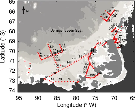
The Bellingshausen Sea is situated to the west of the Antarctic Peninsula between 75◦W and 90◦W and is a transition region between continental shelf, shelf breaks and the open ocean. The sampling period consisted of 38 days between 3 March and 9 April 2007, which represent the seasonal shift from late summer to early autumn (Fig. 1). The hydrographic profiles were taken with a Sea-Bird 911+ CTD package

20

mounted on a rosette with 12 ten-litre Niskin bottles for the collection of water samples. The CTD conductivity sensor was calibrated on board against discrete samples anal-ysed with aGuildline Autosal 8400B. A constant offset of +0.034±0.040 was found

and corrected for. A high-precision reversing thermometer sensor (Sea-Bird SBE35) and an O₂ sensor (CTD-O₂; Sea-Bird SBE43) were also mounted on the rosette.

25

(7)

OSD

8, 1505–1533, 2011

Title Page

Tables Figures

◭ ◮

Back Close

Full Screen / Esc

Discussion

P

a

per

|

Dis

cussion

P

a

per

|

Discussion

P

a

per

|

Discussio

n

P

a

per

|

or about 1 m) to the maximum depth for each station. The CTD-O₂ data were cali-brated against discrete samples analysed on board using whole-bottle Winkler titration (Dickson, 1996) with photometric end-point detection. A total of 276 titrations were performed with a repeatability of 0.29 µmol kg−1 (0.1 %) based on 76 duplicate sam-ples. The average difference between the non-calibrated CTD-O2 and Winkler data

5

was (3.9±3.1) µmol kg−1.

For determiningz_mixusing difference criteria, the sensor precision is more important than the absolute accuracy. The sensor precision was estimated from the relative standard deviation of the CTD-O2readings within 2 dbar-bins in the mixed layer, which was found to be (0.4±0.3) %, on average.

10

2.2 Definition of the zmix(O2) criterion

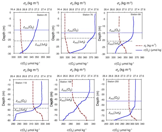
To define a z_mix criterion based on O₂, all 253 CTD profiles were initially inspected visually. Two profiles could not be used due to sensor problems. Some examples of typical profiles encountered during the survey are depicted in Fig. 2. Subjective, visu-ally determinedz_mix was then compared to objective, numerically determined z_mix to

15

identify a suitable O2criterion for zmix. We propose to definezmix(O2) as the depth at whichc(O2) has changed by 0.5 % with respect to a reference value at 10 dbar. Brain-erd and Gregg (1995) suggested 10 dbar as reference depth to avoid sensor noise in the surface water due to the effect of ship motion. Sensor noise affected our measure-ments only in the top 5 dbar of most CTD stations. Using this reference depth means

20

that the minimumz_mix is 10 dbar. The reference depth of 10 dbar was also chosen for consistency with other studies and to allow comparing our results to climatological data that use the same reference depth.

2.3 Comparison with density- and temperature-based zmixand climatologies

Comparisons betweenz_mix(O₂) and z_mix based on temperature and potential density

25

(8)

OSD

8, 1505–1533, 2011

Title Page

Tables Figures

◭ ◮

Back Close

Full Screen / Esc

Discussion

P

a

per

|

Dis

cussion

P

a

per

|

Discussion

P

a

per

|

Discussio

n

P

a

per

criteria used in selected three-widely used climatologies were chosen. A further com-parison was made between ofz_mix(O₂) and the actual z_mix values from the climatolo-gies, interpolated according to location and time of year (Table 1).

Climatologies represent binned and averaged monthly fields. The z_mix climatolo-gies by Monterey and Levitus (1997), Kara et al. (2003) and de Boyer Mont ´egut et

5

al. (2004) (referred to as ML97, K03 and BM04 hereinafter and respectively) are widely used in oceanographic studies. The corresponding data were obtained from http: //www.esrl.noaa.gov/psd/data/gridded/data.nodc.woa94.html, http://www7320.nrlssc. navy.mil/nmld/nmld.html and http://www.locean-ipsl.upmc.fr/∼_{cdblod/mld.html. ML97} and K03 are based on data from the World Ocean Atlas 1994 (WOA94). BM04 is

10

based on individual CTD profiles obtained from the World Ocean Circulation Experi-ment (WOCE) and the National Oceanographic Center (NODC) and the latest update includes profiles from Argo floats. The BM04 climatology is obtained by an ordinary kriging of the data distributed in 2o boxes, with a prediction limited to 1000 km ra-dius. No value is assigned if there are less than 5 data points in a grid box. BM04

15

includes profiles from mechanical bathythermograph (MBT), expendable bathythermo-graph (XBT), CTD hydrocasts and profiling floats, providing a range of vertical reso-lutions from 2.3 m (CTD) to 19.5 m (XBT). The ML97 and K03 climatologies consider a smaller radius of influence (771 km). However, interpolation of data and smoothing were performed within that radius leading to larger uncertainties in the data.

20

Based on ML97 and BM04, the following criteria were chosen to definez_mixbased on potential temperature (θ) and potential density (σ_θ) differences:∆θ₌0.2◦C and∆σ_θ₌ 0.125 kg m−3_{with respect to the surface value;}_∆_θ₌_0.5◦_{C and}_∆_σ

θ=0.03 kg m−

3 with respect to the 10 dbar value. These criteria were applied to the same 251 CTD profiles used to determine z_mix(O2). In addition, zmix(O2) was compared with the

curvature-25

basedz_mixalgorithm of Lorbacher et al. (2006) as well asz_mixbased on the 95 % O₂ saturation criterion (Talley, 1999).

(9)

OSD

8, 1505–1533, 2011

Title Page

Tables Figures

◭ ◮

Back Close

Full Screen / Esc

Discussion

P

a

per

|

Dis

cussion

P

a

per

|

Discussion

P

a

per

|

Discussio

n

P

a

per

|

climatologies suffer from poor data coverage in the Southern Ocean, particularly south of 30◦S in the Antarctic coastal zone, we planned to use a dedicated Southern Ocean z_mixclimatology based onσ_θdifferences derived from Argo float profiles used for com-parison (Dong et al., 2008). However, it turned out that this climatology did not contain any data in the region of study and could therefore not be used.

5

To further test the z_mix(O2) criterion, we applied the ∆σθ=0.03 kg m−

3

criterion to density profiles calculated from 1◦by 1◦-temperature and salinity climatology in World Ocean Atlas 2005 (WOA05; http://www.nodc.noaa.gov/OC5/WOA05/woa05data.html; (Antonov et al., 2006; Locarnini et al., 2006). Then, the z_mix(O2) criterion was ap-plied to the O₂data in WOA05 (Garcia et al., 2006). WOA05 uses the same standard

10

depths and interpolation method for temperature, salinity and oxygen. The O₂ data only comprise results obtained by Winkler titration.

3 Results

3.1 Comparison between zmix(O2) from subjective and objective analysis

z_mix(O₂) obtained by subjective visual inspection and by using objective numerical

anal-15

ysis agreed to within 1 dbar for 235 out of 251 stations. For the remaining 16 stations, the objectivez_mix(O2) value was on average (1±5) dbar shallower than its subjective counterpart (Fig. 3). This small discrepancy was caused by the presence of low oxy-genated subsurface waters (i.e. Winter Water) that created a weak upper oxycline. The visual inspection disregarded this top oxycline andz_mix(O2) was defined according to

20

the deeper and more pronounced seasonal oxycline. In the following, the subjective result is used forz_mix(O2).

Thez_mix(O2) criterion appears to better reflect the O2distribution in the mixed layer, compared to thez_mix(∆σ_θ₌0.03 kg m−3) criterion. This is illustrated by six typical pro-files (Fig. 2). Vertical propro-files for stations 25, 76, 89, 188, 199 and 250, showz_mix(∆σ_θ

25

(10)

OSD

8, 1505–1533, 2011

Title Page

Tables Figures

◭ ◮

Back Close

Full Screen / Esc

Discussion

P

a

per

|

Dis

cussion

P

a

per

|

Discussion

P

a

per

|

Discussio

n

P

a

per

the O2 concentration is lower atzmix(∆σθ=0.03 kg m−

3

) than at z_mix(O2). This diff er-ence can lead to an underestimation of the average mixed layer O2concentration.

3.2 Comparison between zmix(O2) and zmixbased onθ andσθ differences

No significant correlation was observed between z_mix(O2) and zmix based on

∆θ₌0.5◦C (with respect to the surface value) or based on∆θ₌0.2◦C (with respect

5

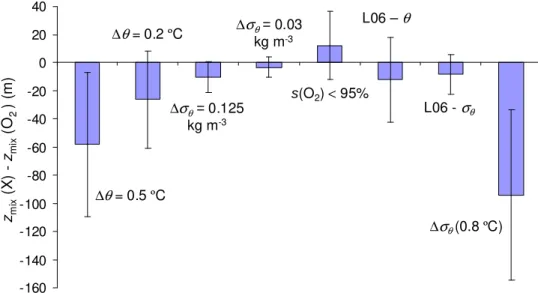
to the 10 dbar value). The corresponding correlation coefficients were r2₌0.001 and 0.111, respectively. z_mix(_∆θ₌0.5◦_{C) was on average (58}

±51) dbar deeper than

z_mix(O2), whilezmix(∆θ=0.2◦C) was (26±34) dbar deeper. These observations con-firm the overestimation ofz_mixbased on temperature in the Southern Ocean providing the importance of using density to definez_mixin this area (Figs. 4 and 5a).

10

Comparison betweenz_mix(O2) andzmixbased on∆σθ=0.125 kg m−

3

with respect to the surface value,∆σ_θ₌0.03 kg m−3 and∆σ_θ due to a temperature change of 0.8◦C,

∆σ_θ(0.8◦_C)₌_σ

θ (θ+0.8◦C) – σθ (θ), both with respect to the 10 dbar value, showed

a better agreement than for the solelyθ–based criteria. The corresponding correlation coefficients werer2₌0.711, 0.813 and 0.016, respectively. z_mix(∆σ_θ₌0.125 kg m−3)

15

was on average (14±13) dbar deeper thanzmix(O2), whilezmix(∆σθ=0.03 kg m−

3 ) was (3±7) dbar deeper and zmix(∆σθ(0.8◦C)) was (94±60) dbar deeper (Figs. 4 and 5b).

We also confirmed the results obtained based on the∆σ_θ criteria visually. Objective and subjective results agreed to within (2±6) dbar for all criteria.

Lorbacher et al. (2006) have defined z_mix based on the first extreme curvature in

20

the temperature or potential density profile. Compared to difference criteria, this ap-proach has the advantage of being independent of the actual value of the variable in question. The same is true forz_mix(O2), which uses a relative difference of 0.5 %, independent of the O2 concentration. The mixed layer depth based on temperature curvature, z_mix(θ′′), gave (12±30) dbar deeper values than zmix(O2); zmix based on

25

(11)

OSD

8, 1505–1533, 2011

Title Page

Tables Figures

◭ ◮

Back Close

Full Screen / Esc

Discussion

P

a

per

|

Dis

cussion

P

a

per

|

Discussion

P

a

per

|

Discussio

n

P

a

per

|

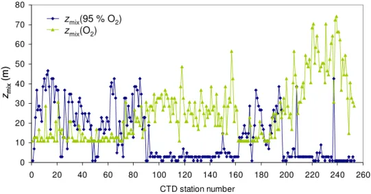
Talley (1999) used the 95 % O₂-saturation horizon to identify winter mixed layer depth. We tested this criterion to identify summer/autumn mixed layer depth during our cruise. Away from the shore (stations 90 to 163 and 197 to 253), the 95 % saturation criterion does not give meaningful results because of the presence O₂-undersaturated waters near the surface. Closer to ice shelves (stations 1 to 90 and 166 to 198),

bio-5

logical production is able to overcome this O2 deficit. The surface O2 saturation was (100±4) % and zmix(95 % O2) was on average (12±24) dbar deeper than zmix(O2) (Fig. 6).

3.3 Comparison of z_mixwith climatologies

For the following comparisons, the z_mix data are presented in meters (rather than

10

dbar) to keep consistent with the climatologies. Comparison between z_mix from the selected criteria with the z_mix obtained from the same criteria according to the cor-responding climatology was done. This means that the z_mix(∆σ_θ₌0.125 kg m−3), z_mix(∆σ_θ₌0.03 kg m−3) andz_mix(∆σ_θ(0.8◦C)) derived from our profiles was compared with the corresponding values extracted from the ML97, BM04 and K03 climatologies,

15

respectively, for the same month and location were done. Due to the limited spatial cov-erage of the climatologies in the Southern Ocean, not all profiles had a corresponding climatologicalz_mixvalue (170 profiles for ML97, 208 profiles for BM04 and 179 profiles for K03 all out of 251). Therefore, the comparisons below were done for the common minimum number of profiles found in the climatologies.

20

The ML97 and K03 climatologies have a coarse vertical resolution (0, 10, 20, 30, 50, 75, 100, 125, 150, 200, 250, 300, 400, 500, 600, 700, 800, 900, 1000 m), which puts limits on the comparison to in situz_mixdata based on profiles with 2 dbar resolution. For some CTD stations, climatologicalz_mixwas overestimated by up to 500 m with respect toz_mix(O2). These values were disregarded for the comparison between climatological

25

(12)

OSD

8, 1505–1533, 2011

Title Page

Tables Figures

◭ ◮

Back Close

Full Screen / Esc

Discussion

P

a

per

|

Dis

cussion

P

a

per

|

Discussion

P

a

per

|

Discussio

n

P

a

per

Comparisons with z_mix from ML97 and B04 showed a good agreement, with r2₌ 0.628 for ML97 andr2₌0.604 for BM04 (data not shown). The ML97 climatology gave (11.9±11.6) m shallower zmix than the in situ data; the BM04 climatology gave (0.7

±13.5) m shallower zmix. However, zmix(∆σθ(0.8 ◦C)) showed poor agreement with

the corresponding data from K03 (r2₌0.002), withz_mix based on CTD profiles being

5

(94.4±64.1) m deeper.

We then comparedz_mix(O2) with the density-basedzmixin the BM04, ML97 and K03 climatologies. To ensure comparable results, we only used the profiles where data from all climatologies were available, so that the total number of profiles compared was 160 (Table 2). z_mix(∆σ_θ₌0.03 kg m−3) from BM04 showed a positive

correla-10

tion with z_mix(O2) (r 2

=0.542) and was on average (6±11) m deeper than zmix(O2).

z_mix(∆σ_θ₌0.125 kg m−3) from ML97 also showed a positive correlation with z_mix(O2) (r2 ₌0.542), and was on average (1±11) m shallower than zmix(O2). No correlation was found betweenz_mix from K03 and z_mix(O2), withzmix(O2) on average (15±14) m deeper (Table 2).

15

Our observations show thatz_mix(_∆σ_θ₌0.03 kg m−3_{) is most similar to}_z

mix(O2). The BM04 climatology showed the best coverage in the Southern Ocean, and has the ad-vantage of having a higher vertical resolution than to the other climatologies.

3.4 zmix(O2) compared with zmixbased on WOA05 density and oxygen profiles

The criterionz_mix(∆σ_θ₌0.03 kg m−3) was applied to density profiles taken from

objec-20

tively analysed fields of temperature and salinity data from WOA05. We then compared the results obtained from these observations to thez_mixusing the same density crite-rion and the oxygen critecrite-rion both in our CTD profiles. For the WOA05 profiles we could only find matching data for 120 out of 251 CTD profiles, due to the limited spatial cov-erage of WOA05. A poor correlation was found for both comparisons (r2₌0.048 and

25

(13)

OSD

8, 1505–1533, 2011

Title Page

Tables Figures

◭ ◮

Back Close

Full Screen / Esc

Discussion

P

a

per

|

Dis

cussion

P

a

per

|

Discussion

P

a

per

|

Discussio

n

P

a

per

|

deeper than based on WOA05. These differences are likely due to the scarce WOA05 data in the Southern Ocean and their limited vertical resolution (10 m) (Table 2).

To test thez_mix(O2) criterion with other O2profiles, we used historical O2profiles from WOA05 located at the same geographical location than our CTD stations. Our results show a positive correlation (r2₌0.412) betweenz_mix(CTD-O2) and zmix(WOA05-O2).

5

On average,z_mix(WOA05-O2) was (8±12) dbar shallower thanzmix(CTD-O2).

4 Discussion

Definingz_mixbased on potential temperature can lead to deeper values thanz_mix(O₂), which is defined based on the vertical O2distribution. The∆θ=0.5◦C and∆θ=0.2◦C

criteria lead toz_mix located within the oxycline. These criteria tend to underestimate

10

the average mixed layer O₂ concentration. Potential density-based z_mix values are in better agreement withz_mix(O2), particularly for the∆σθ=0.03 kg m−

3

criterion.

To explain the discrepancy between temperature and density-based z_mix, we checked for the presence of barrier layers and temperature inversions in the area of study. Barrier layers are thought to be formed by melting sea ice, although the

mech-15

anisms for the formation and destruction of barrier layers in the Southern Ocean are not well understood (de Boyer Mont ´egut et al., 2007). Our results showed that barrier layers were present in 43 % of the CTD profiles. The barrier layer thickness ranged from 2 to 93 m. Barrier layers were also encountered below the seasonal mixed layer, but do not influencez_mix(O₂). The seasonal variability of the barrier layers, influenced

20

mainly by the water column stratification, is expected to correspond to that ofz_mix(O2). The deepening ofz_mixduring autumn and winter will lead to low-O2waters entering the ML from the barrier layer below and subsequent destruction of the barrier layer.

Comparison between in situz_mix(O2) withzmixclimatologies showed a good agree-ment for the ML97 and BM04 climatologies. BM04 has several advantages over

25

(14)

OSD

8, 1505–1533, 2011

Title Page

Tables Figures

◭ ◮

Back Close

Full Screen / Esc

Discussion

P

a

per

|

Dis

cussion

P

a

per

|

Discussion

P

a

per

|

Discussio

n

P

a

per

non-averaged profiles, which avoids the creation of artificially smooth profiles as in ML97 and K03; (3) ML97 and K03 have limited vertical resolution and use discrete intervals; (4) non-averaged profiles allow identification of upper water structures such as barrier layers and temperature inversions; (5) a difference-criterion based on tem-perature or density with a wide threshold (such as in ML97 and K03), can lead to an

5

overestimation ofz_mix. De Boyer Mont ´egut et al. (2004) reasoned that a wider threshold might be better for averaged-profiles with a coarser and smoother resolution.

Both the ML97 and K03 temperature criteria have been applied for areas where sharp temperature stratification in the upper water column is present (i.e. tropical and sub-tropical oceanic areas). The larger temperature difference of the K03 criterion

10

producesz_mixvalues higher than those of ML97.

Argo float data such as used in the latest update of the BM04 climatology provide new insights for seasonalz_mix investigations in a region where the lack of data during austral winter from direct observations collected on board research ships is consider-able. Argo floats with O2sensors have been launched since 2007, a few of them in the

15

Southern Ocean. However, these floats are only located in deep waters and the coarse vertical resolution that the Argo profiles provide (≈10.5 m) are important limitations for

detection of shallow summer z_mix in the coastal region of the Southern Ocean. Due to this, the climatology by Dong et al. (2008) is limited to 30◦S to 65◦S excluding the location of the Bellingshausen Sea (i.e. 66◦_{S to 74}◦_S).

20

z_mix based on curvature as proposed by Lorbacher et al. (2006) showed a similar overestimation ofz_mix(O2) as the density and temperature criteria. Although the L06 criterion does not require a common vertical resolution between analysed profiles, this criterion was created from monthly means data and may therefore not work for single profiles as in our case. The L06 criterion however has the advantage of being

inde-25

pendent of the actual value of the variable in question. This is also true for thez_mix(O₂) which uses a relative difference of 0.5 % independent of the oxygen concentrations.

The 95 % O2 saturation criterion proposed by Talley (1999) gives mostly lower

(15)

OSD

8, 1505–1533, 2011

Title Page

Tables Figures

◭ ◮

Back Close

Full Screen / Esc

Discussion

P

a

per

|

Dis

cussion

P

a

per

|

Discussion

P

a

per

|

Discussio

n

P

a

per

|

because the physical and biogeochemical processes would not appear to be compa-rable enough from place to place and time to time to allow using such an “absolute” horizon.

The nighttime convection and overturning have a daily effect on thez_mixwith higher values as the wind speed increases during the night. This effect might also yield a

5

differential response of gas fluxes due to diurnal thermocline variations. From the to-tal CTD profiles evaluated here in the continento-tal shelf of the Bellingshausen Sea, 17 % (43 stations) were sampled during the period of darkness (about 5 h; from 23:00 to 04:00 LT). From the observations in Fig. 7, there is no clear difference be-tween z_mix during the night and day either using O2 or the potential density criterion

10

(i.e.∆σ_θ₌0.03 kg m−3). This may be expected because nighttime convection is likely to be limited during summer (and early autumn). In order to evaluate in detail the e_ffect of nighttime convection onz_mix(O2), in situ measurements of the vertical profile of O2in a daily time series at the same geographical location are needed. High variability due to diurnal e_ffects has been investigated before for oxygen isotopes in dissolved water

15

from Sagami Bay, Japan (Sarma et al., 2006). The authors found that the distribution of oxygen isotopes is strongly influenced by diurnal variability. This effect would also influence of production calculations, but can be neglected for our study.

The accuracy ofz_mix depends on the resolution of the instrumental parameter used in the criterion to define it. By using CTD observations, the resolution is sufficiently high

20

to identify the vertical distribution of O₂in the upper water column, and therefore define an adequatez_mix in a less coarse vertical resolution than the integrated observations byz_mix climatologies and WOA data. The low abundance of O2 profiles in the WOA record for the Southern Ocean make z_mix obtained from these data sets unreliable when compared to the in situz_mix values based on CTD-O2 profiles. Moreover, the

25

(16)

OSD

8, 1505–1533, 2011

Title Page

Tables Figures

◭ ◮

Back Close

Full Screen / Esc

Discussion

P

a

per

|

Dis

cussion

P

a

per

|

Discussion

P

a

per

|

Discussio

n

P

a

per

Finally, despite in this work the O₂ concentrations from the CTD profiles were pre-viously calibrated against results from Winkler method, the z_mix obtained after the z_mix(O2) criterion can be also applied directly to non-calibrated vertical profiles, pro-vided bad data such as spikes are removed from the O₂profiles.

5 Conclusions

5

The O₂concentration in the coastal Southern Ocean is a better parameter to definez_mix for gas exchange studies. For profiles in the Bellingshausen Sea collected during late summer and autumn in 2007, thez_mixwas well defined by the depth where the absolute di_fference in the concentration of O₂ was higher than 0.5 % of the concentration at 10 dbar depth. The criterion was validated by further visual inspection with 94 % of the

10

total working profiles agreeing well with the proposed criterion.

In coastal waters of the Southern Ocean, the vertical stratification of salinity is a delimiting factor for the upper water dynamics due to the strong ice-melting water sig-nal. After validation of the z_mix obtained from O2 against the zmix obtained from tra-ditional potential density and temperature criteria, it was found a best agreement with

15

the∆σ_θ₌0.03 kg m−3criterion, applied to the CTD profiles and with the corresponding z_mixextracted from the monthly climatology (BM04) (de Boyer Mont ´egut et al., 2004).

Thus, in the absence of O₂ profiles, the z_mix(∆σ_θ₌0.03 kg m−3) criterion might be used. Furthermore, in the absence of CTD stations at all, the public monthly clima-tology BM04 (de Boyer Mont ´egut et al., 2004), based on the same∆σ_θ-criterion, is

20

encouraged to be used for determination ofz_mix in the coastal areas of the Southern Ocean.

For gas exchange studies, z_mix(O2) has the advantage of being directly related to a species of interested. Moreover, the relative nature ofz_mix(O₂) criterion means that it should be applicable in many other parts of the worlds’ oceans, including during

25

(17)

OSD

8, 1505–1533, 2011

Title Page

Tables Figures

◭ ◮

Back Close

Full Screen / Esc

Discussion

P

a

per

|

Dis

cussion

P

a

per

|

Discussion

P

a

per

|

Discussio

n

P

a

per

|

or determination of marine production using dissolved gases as proxy in the coastal Southern Ocean, the use of thez_mix(O₂) criterion is suggested. The proposed criterion is more sensitive to reflect better upper mixed layer air-sea dynamics and influence of biological and physical processes, rather than the traditional criteria based on po-tential temperature or density, particularly in regions where weak vertical gradients of

5

temperature and density in the upper waters are suspected.

Acknowledgements. The British Antarctic Survey (BAS) and the Natural Environment Re-search Council supported this project through grant CGS8/29. K. C. M. thanks the National Council for Science and Technology (CONACyT), Mexico, for her PhD scholarship at the Uni-versity of East Anglia. J. K. was also supported by a Royal Society Research Merit Award 10

(WM052632). Our thanks extend to the principal scientist, Deborah Shoosmith, and the other participants and crew of cruise JR165, as well as the leader of the ACES-FOCAS project, Adrian Jenkins.

References

Antonov, J. I., Locarnini, R. A., Boyer, T. P., Mishonov, A. V., and Garc´ıa, H. E.: Salinity, in: 15

World Ocean Atlas, 2005, edited by: Levitus, S., NOAA Atlas NESDIS 62, U.S Government Printing Office, Washington, D. C., 182, 2006.

Arrigo, K. R., van Dijken, G. L., and Bushinsky, S.: Primary production in the Southern Ocean, 1997–2006, J. Geophys. Res., 113, 1–27, doi:10.1029/2007JC004551, 2008.

Brainerd, K. E. and Gregg, M. C.: Surface mixed and mixing layer depths, Deep-Sea Res. Pt. I, 20

42, 1177–1200, doi:10.1016/0967-0637(95)00068-H, 1995.

Cisewski, B., Strass, V. H., Losch, M., and Prandke, H.: Mixed layer analysis of a mesoscale eddy in the Antarctic Polar Front Zone, J. Geophys. Res., 113, 1–19, doi:10.1029/2007JC004372, 2008.

de Boyer Mont ´egut, C., Madec, G., Fisher, A. S., Lazar, A., and Iudicone, D.: Mixed layer 25

depth over the global ocean: an examination of profile data and profile-based climatology, J. Geophys. Res., 109, 1–20, doi:10.1029/2004JC002378, 2004.

(18)

OSD

8, 1505–1533, 2011

Title Page

Tables Figures

◭ ◮

Back Close

Full Screen / Esc

Discussion

P

a

per

|

Dis

cussion

P

a

per

|

Discussion

P

a

per

|

Discussio

n

P

a

per

mixed layer depth in the world ocean: 1. General description, J. Geophys. Res., 112, 1– 12, doi:10.1029/2006JC003953, 2007.

Dong, S., Sprintall, J., Gille, S. T., and Talley, L.: Southern Ocean mixed-layer depth from Argo float profiles, J. Geophys. Res., 113, 1–12, doi:10.1029/2006JC004051, 2008.

Ducklow, H. W., Fraser, W., Karl, D. M., Quetin, L. B., Ross, R. M., Smith, R. C., Stammerjohn, 5

S., Vernet, M., and Daniels, R. M.: Water-column processes in the West Antarctic Peninsula and the Ross Sea: Interannual variations and foodweb structure, Deep-Sea Res. Pt. II, 53, 834–852, doi:10.1016/j.dsr2.2006.02.009, 2006.

Fairall, C. W., Hare, J. E., Edson, J. B., and McGillis, W.: Parameterization and microm-eteorological measurement of air-sea gas transfer, Bound-Lay. Meteorol., 96, 63–105, 10

doi:10.1023/A:1002662826020, 2000.

Garcia, H. E. and Keeling, R. F.: On the global oxygen anomaly and air-sea flux, J. Geophys. Res., 106, 31155–31166, doi:10.1029/1999JC000200, 2001.

Garcia, H. E., Locarnini, R. A., Boyer, T. P., and Antonov, J. I.: Dissolved Oxygen, Apparent Oxygen Utilization and Oxygen Saturation, in: World Ocean Atlas, 2005, edited by: Levitus, 15

S., NOAA Atlas NESDIS 63, U.S Government Printing Office, Washington, D.C., 342, 2006. Gordon, A. L. and Huber, B. A.: Southern Ocean winter mixed layer, J. Geophys. Res., 95,

11655–11672, doi:10.1029/JC095iC07p11655, 1990.

Holte, J. and Talley, L.: A new algorithm for finding mixed layer depths with applications to Argo data and Subantarctic Mode Water Formation, J. Atmos. Ocean. Tech., 29, 1920–1939, 20

doi:10.1175/2009JTECHO543.1, 2009.

Jenkins, A. and Jacobs, S. S.: Circulation and melting beneath George VI Ice Shelf, Antarctica, J. Geophys. Res., 113, 1–18, doi:10.1029/2007JC004449, 2008.

Kaiser, J., Reuer, M. K., Barnett, B., and Bender, M. L.: Marine productivity estimates from con-tinuous oxygen/argon ratio measurements by shipboard membrane inlet mass spectrometry, 25

Geophys. Res. Lett., 32, L19605, doi:19610.11029/12005GL023459, 2005.

K ¨ortzinger, A., Send, U., Wallace, D. W. R., Karstensen, J., and DeGrandpre, M.: Seasonal cycle of O₂ andpCO₂ in the central Labrador Sea: Atmospheric, biological, and physical implications, Global Biogeochem. Cy., 22, 1–16, doi:10.1029/2007GB003029, 2008.

Le Qu ´er ´e, C., Aumont, O., Monfray, P., and Orr, J. C.: Propagation of climatic events on ocean 30

stratification, marine biology, and CO₂: case studies over the 1979–1999 period, J. Geophys. Res., 108, 1–7, doi:10.1029/2001JC000920, 2003.

(19)

OSD

8, 1505–1533, 2011

Title Page

Tables Figures

◭ ◮

Back Close

Full Screen / Esc

Discussion

P

a

per

|

Dis

cussion

P

a

per

|

Discussion

P

a

per

|

Discussio

n

P

a

per

|

Locarnini, R. A., Mishonov, A. V., Antonov, J. I., Boyer, T. P., and Garc´_ıa, H. E.: Temperature, in: World Ocean Atlas, 2005, edited by: Levitus, S., NOAA Atlas NESDIS 61, U.S. Government Printing Office, Washington, D.C., 182, 2006.

Lorbacher, K., Dommenget, D., Niiler, P., and K ¨ohl, A.: Ocean mixed layer depth: A subsurface proxy of ocean-atmosphere variability, J. Geophys. Res., 111, 1–22, 5

doi:10.1029/2003JC002157, 2006.

Lukas, R. and Lindstrom, E.: The mixed layer of the western equatorial Pacific Ocean, J. Geophys. Res., 96, 3343–3357, 1991.

Noh, Y., and Lee, W.: Mixed and mixing layer depths simulated by and OGCM, J. Oceanogr., 64, 217–225, doi:10.1007/s10872-008-0017-1, 2008.

10

Reuer, M. K., Barnett, B. A., Bender, M. L., Falkowski, P. G., and Hendricks, M. B.: New estimates of Southern Ocean biological production rates from O₂/Ar ratios and the triple isotope composition of O₂, Deep-Sea Res. Pt. I, 54, 951–974, 2007.

Rintoul, S. R. and Trull, T. W.: Seasonal evolution of the mixed layer in the Subantarctic Zone south of Australia, J. Geophys. Res., 106, 31447–31462, doi:10.1029/2000JC000329, 2001. 15

Sarma, V. V. S. S., Abe, O., Hinuma, A., and Saino, T.: Short-term variation of triple oxygen isotopes and gross oxygen production in the Sagami Bay, central Japan, Limnol. Oceanogr., 51, 1432–1442, doi:10.4319/lo.2006.51.3.1432, 2006.

Smith, R. C., Martinson, D. G., Stammerjohn, S. E., Iannuzzi, R. A., and Ireson, K.: Belling-shausen and western Antarctic Peninsula region: Pigment biomass and sea-ice spa-20

tial/temporal distributions and interannual variabilty, Deep-Sea Res. Pt. II, 55, 1949–1963, doi:10.1016/j.dsr2.2008.04.027, 2008.

Talley, L.: Some aspects of ocean heat transport by the shallow, intermediate and deep over-turning circulations, in: Mechanisms of Global Climate Change at Millennial Time Scales, edited by: Clark, P. U., Webb, R. S., and Keigwin, L. D., Geophysicall Monograph, American 25

Geophysical Union, Washington, D.C., 1–22, 1999.

Thomson, R. E. and Fine, I. V.: Estimating mixed layer depth from oceanic profile data, J. Atmos. Ocean. Tech., 20, 319–329, doi:10.1175/1520-0426(2003)020<0319:EMLDFO>2.0.CO;2, 2003.

Verdy, A., Dutkiewicz, S., Follows, M. J., Marshall, J., and Czaja, A.: Carbon dioxide and oxygen 30

(20)

OSD

8, 1505–1533, 2011

Title Page

Tables Figures

◭ ◮

Back Close

Full Screen / Esc

Discussion

P

a

per

|

Dis

cussion

P

a

per

|

Discussion

P

a

per

|

Discussio

n

P

a

per

Williams, G. D., Nicol, S., Raymond, B., and Meiners, K.: Summertime mixed layer development in the marginal sea ice zone offthe Mawson coast, East Antarctica, Deep-Sea Res. Pt. II, 55, 365-376, doi:10.1016/j.dsr2.2007.11.007, 2008.

Zawada, D. G., Roland, J., Zaneveld, V., and Boss, E.: A comparison of hydro-graphically and optically derived mixed layer depths, J. Geophys. Res., 110, 1–13, 5

(21)

OSD

8, 1505–1533, 2011

Title Page

Tables Figures

◭ ◮

Back Close

Full Screen / Esc

Discussion

P

a

per

|

Dis

cussion

P

a

per

|

Discussion

P

a

per

|

Discussio

n

P

a

per

|

Table 1.Climatologies used in this work to compare with the mixed layer depths extracted from O₂profiles.

Abbreviation Authors Description Data source2 _Profiles _Resolution _Criteria _Reference

depth

ML97 Monterey and Levitus (1997) zmixclimatology WOA94

(1900–1992)

averaged, interpolated

1◦

×1◦ monthly

∆σθ=0.5 g m−3

and∆θ=0.5◦_C

0 m

K03 Kara et al. (2003) zmixclimatology WOA94

(1900–1992)

1◦

×1◦ monthly

∆σθ corresponding

to∆θ=0.8◦_C

0 m

BM04 de Boyer Mont ´egut et al. (2004)

and LOCEAN-IPSL1₍₂₀₀₈₎

zmixclimatology NODC/WOCE/Argo

(1941–2008)

individual 2◦

×2◦ monthly

∆σθ=0.03 kg m−3

and∆θ=0.2◦_C

10 m

WOA05-σθ This work TandSclimatology WOA

(1965–2005)

1◦

×1◦ monthly

∆σθ=0.03 kg m−3 10 m

WOA05-O2 This work c(O2) climatology WOA

(1965–2005)

1◦_×₁◦

monthly

∆s(O2)=0.5 % 10 m

1_{Laboratoire d’Oc éanographie et de Climatologie par l’Exp érimentation et l’Analyse Num érique – Institut Pierre Simon} Laplace (updated version from the previously published by de Boyer Mont égut et al., 2004).

(22)

OSD

8, 1505–1533, 2011

Title Page

Tables Figures

◭ ◮

Back Close

Full Screen / Esc

Discussion

P

a

per

|

Dis

cussion

P

a

per

|

Discussion

P

a

per

|

Discussio

n

P

a

per

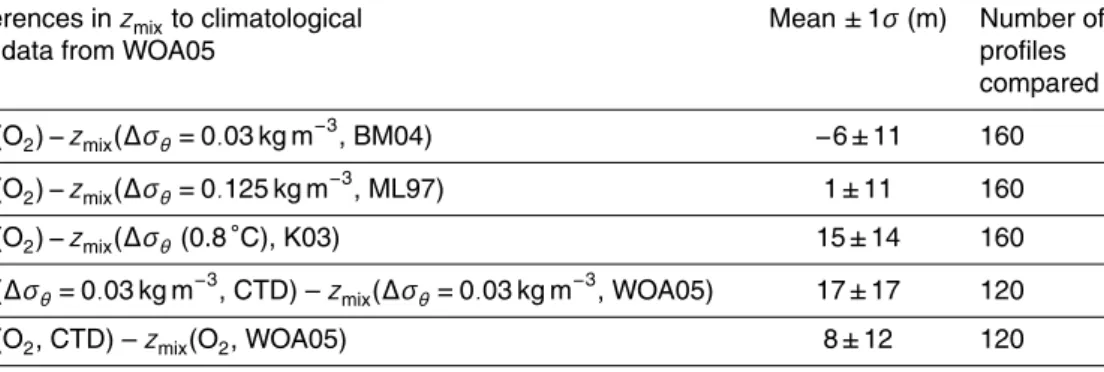
Table 2. Mean (±1σ) difference fromz_mix(O₂) in CTD and World Ocean Atlas 2005 (WOA05) profiles to data from climatologies and WOA05 based on∆σ_θ.

Differences inz_mixto climatological and data from WOA05

Mean±1σ(m) Number of profiles compared

z_mix(O₂)−z_mix(∆σ_θ=0.03 kg m−3_{, BM04)}

−6±11 160

z_mix(O2)−zmix(∆σθ=0.125 kg m−

3

, ML97) 1±11 160

z_mix(O₂)−zmix(∆σθ(0.8◦C), K03) 15±14 160

z_mix(∆σ_θ=0.03 kg m−3

, CTD) –z_mix(∆σ_θ=0.03 kg m−3

, WOA05) 17±17 120

(23)

OSD

8, 1505–1533, 2011

Title Page

Tables Figures

◭ ◮

Back Close

Full Screen / Esc

Discussion

P

a

per

|

Dis

cussion

P

a

per

|

Discussion

P

a

per

|

Discussio

n

P

a

per

|

95 90 85 80 75 70 65

Longitude (

_º

W)

65

66

67

68

69

70

71

72

73

74 L

a

ti

tu

d

e

(

º

S)

95 90 85 80 75 70 65

Longitude (

_º

W)

65

66

67

68

69

70

71

72

73

74 L

a

ti

tu

d

e

(

º

S)

(24)

OSD

8, 1505–1533, 2011

K. Castro-Morales and J. Kaiser Title Page Abstract Introduction Conclusions References Tables Figures ◭ ◮ ◭ ◮ Back Close

Full Screen / Esc

Printer-friendly Version Interactive Discussion Discussion P a per | Dis cussion P a per | Discussion P a per | Discussio n P a per Station 25

σ_θ(kg m-3 ) 26.4 26.6 26.8 27.0 27.2 27.4 27.6

-30 -25 -20 -15 -10 -5 0 MLD-O2

MLD-σθ

Station 76

σ_θ (kg m-3 ) 26.4 26.6 26.8 27.0 27.2 27.4 27.6

D e p th (d b a r) -30 -25 -20 -15 -10 -5 0 MLD-O2

MLD-σθ

Station 89

σ_θ (kg m-3 ) 26.4 26.6 26.8 27.0 27.2 27.4 27.6

D e p th (d b a r) -30 -25 -20 -15 -10 -5 0 MLD-O2

MLD-σθ

σθ(kg m-3)

26.4 26.6 26.8 27.0 27.2 27.4 27.6

σθ(kg m-3)

26.4 26.6 26.8 27.0 27.2 27.4 27.6

σθ(kg m-3)

26.4 26.6 26.8 27.0 27.2 27.4 27.6

D e p th ( m ) 0 -5 -10 -15 -20 -25 -30 D e p th ( m ) 0 -5 -10 -15 -20 -25 -30 330 335 340 345 350 355 360

c(O2) µmol kg-1

0 -5 -10 -15 -20 -25 -30

320 330 340 350 360 370 380

c(O2) µmol kg-1

320 330 340 350 360 370 380

c(O2) µmol kg-1

D e p th ( m )

σθ (kg m-3)

c(O2) (µmol kg -1₎

Station 118

σ_θ (kg m-3 ) 26.4 26.6 26.8 27.0 27.2 27.4 27.6

-80 -70 -60 -50 -40 -30 -20 -10 0

c(O2) (µmol kg

-1₎

280 290 300 310 320 330 340

MLD-O2

MLD-σθ

Station 199

σ_θ (kg m-3 ) 26.4 26.6 26.8 27.0 27.2 27.4 27.6

D e p th (d b a r) -80 -70 -60 -50 -40 -30 -20 -10 0

c(O2) (µmol kg

-1₎

260 280 300 320 340

MLD-O2

MLD-σθ

Station 250

σ_θ (kg m-3 ) 26.4 26.6 26.8 27.0 27.2 27.4 27.6

D e p th ( d b a r) -80 -70 -60 -50 -40 -30 -20 -10 0

c(O2) (µmol kg

-1 )

200 220 240 260 280 300 320 340

MLD-O2

MLD-σθ

σθ(kg m-3)

26.4 26.6 26.8 27.0 27.2 27.4 27.6

D e p th ( m )

280 290 300 310 320 330 340

c(O2) µmol kg-1

0 -10 -20 -30 -40 -50 -60 -70 -80

σθ(kg m-3)

26.4 26.6 26.8 27.0 27.2 27.4 27.6

260 280 300 320 340

c(O2) µmol kg-1

0 -10 -20 -30 -40 -50 -60 -70 -80

σθ(kg m-3)

26.4 26.6 26.8 27.0 27.2 27.4 27.6

200 220 240 260 280 300 320 340

c(O2) µmol kg-1

D e p th ( m ) 0 -10 -20 -30 -40 -50 -60 -70 -80

zmix(O2)

zmix(∆σθ)

zmix(O2) zmix(O2)

zmix(O2)

zmix(∆σθ)

D e p th ( m )

zmix(∆σθ)

zmix(∆σθ) Station 25

σ_θ(kg m-3 ) 26.4 26.6 26.8 27.0 27.2 27.4 27.6

-30 -25 -20 -15 -10 -5 0 MLD-O2

MLD-σθ

Station 76

σ_θ (kg m-3 ) 26.4 26.6 26.8 27.0 27.2 27.4 27.6

D e p th (d b a r) -30 -25 -20 -15 -10 -5 0 MLD-O2

MLD-σθ

Station 89

σ_θ (kg m-3 ) 26.4 26.6 26.8 27.0 27.2 27.4 27.6

D e p th (d b a r) -30 -25 -20 -15 -10 -5 0 MLD-O2

MLD-σθ

σθ(kg m-3)

26.4 26.6 26.8 27.0 27.2 27.4 27.6

σθ(kg m-3)

26.4 26.6 26.8 27.0 27.2 27.4 27.6

σθ(kg m-3)

26.4 26.6 26.8 27.0 27.2 27.4 27.6

D e p th ( m ) 0 -5 -10 -15 -20 -25 -30 D e p th ( m ) 0 -5 -10 -15 -20 -25 -30 330 335 340 345 350 355 360

c(O2) µmol kg-1

0 -5 -10 -15 -20 -25 -30

320 330 340 350 360 370 380

c(O2) µmol kg-1

320 330 340 350 360 370 380

c(O2) µmol kg-1

D e p th ( m )

σθ (kg m-3)

c(O2) (µmol kg -1₎

Station 118

σ_θ (kg m-3 ) 26.4 26.6 26.8 27.0 27.2 27.4 27.6

-80 -70 -60 -50 -40 -30 -20 -10 0

c(O2) (µmol kg

-1₎

280 290 300 310 320 330 340

MLD-O2

MLD-σθ

Station 199

σ_θ (kg m-3 ) 26.4 26.6 26.8 27.0 27.2 27.4 27.6

D e p th (d b a r) -80 -70 -60 -50 -40 -30 -20 -10 0

c(O2) (µmol kg

-1₎

260 280 300 320 340

MLD-O2

MLD-σθ

Station 250

σ_θ (kg m-3 ) 26.4 26.6 26.8 27.0 27.2 27.4 27.6

D e p th ( d b a r) -80 -70 -60 -50 -40 -30 -20 -10 0

c(O2) (µmol kg

-1 )

200 220 240 260 280 300 320 340

MLD-O2

MLD-σθ

σθ(kg m-3)

26.4 26.6 26.8 27.0 27.2 27.4 27.6

D e p th ( m )

280 290 300 310 320 330 340

c(O2) µmol kg-1

0 -10 -20 -30 -40 -50 -60 -70 -80

σθ(kg m-3)

26.4 26.6 26.8 27.0 27.2 27.4 27.6

260 280 300 320 340

c(O2) µmol kg-1

0 -10 -20 -30 -40 -50 -60 -70 -80

σθ(kg m-3)

26.4 26.6 26.8 27.0 27.2 27.4 27.6

200 220 240 260 280 300 320 340

c(O2) µmol kg-1

D e p th ( m ) D e p th ( m ) 0 -10 -20 -30 -40 -50 -60 -70 -80

zmix(O2)

zmix(∆σθ)

zmix(O2) zmix(O2)

zmix(O2)

zmix(∆σθ)

D e p th ( m )

zmix(∆σθ)

Fig. 2. Vertical profiles of O₂ concentration, c(O₂), and potential density (dashed line, σ_θ). Horizontal lines indicate the location of the z_mix defined by c(O₂) and σ_θ after the criterion

(25)

OSD

8, 1505–1533, 2011

Title Page

Tables Figures

◭ ◮

Back Close

Full Screen / Esc

Discussion

P

a

per

|

Dis

cussion

P

a

per

|

Discussion

P

a

per

|

Discussio

n

P

a

per

|

0 10 20 30 40 50 60

0 20 40 60 80 100 120 140 160 180 200 220 240 260

CTD station number

[o

b

je

c

ti

v

e

s

u

b

je

c

it

v

e

]

zm

ix

(O

2

)

(d

b

a

r)

(26)

OSD

8, 1505–1533, 2011

Full Screen / Esc

Printer-friendly Version Interactive Discussion Discussion P a per | Dis cussion P a per | Discussion P a per | Discussio n P a per -160 -140 -120 -100 -80 -60 -40 -20 0 20 40 Me a n d if fe re n c e f ro m ML D -O 2 ( m ) zm ix (X ) -zm ix (O 2 ) (m )

∆θ= 0.2 ºC

L06 -σ_θ

∆θ= 0.5 ºC

∆σθ=0.125 kg m-3

∆σθ=0.03

kg m-3

L06 –θ

s(O2) <95%

∆σθ(0.8 ºC)

-160 -140 -120 -100 -80 -60 -40 -20 0 20 40 Me a n d if fe re n c e f ro m ML D -O 2 ( m ) zm ix (X ) -zm ix (O 2 ) (m )

∆θ= 0.2 ºC

L06 -σ_θ

∆θ= 0.5 ºC

∆σθ=0.125 kg m-3

∆σθ=0.03

kg m-3

L06 –θ

s(O2) <95%

∆σθ(0.8 ºC)

Fig. 4. Mean difference betweenz_mix based on potential temperature and salinity differences or oxygen saturation state (z_mix(X)) to z_mix(O₂). Lorbacher et al. (2006) is the algorithm used by Lorbacher et al. (2006) to definez_mixbased on potential temperature (L06-θ) and potential density (L06-σ_θ). The _∆σ_θ(0.8◦_{C) criterion is based on the di}

(27)

OSD

8, 1505–1533, 2011

Full Screen / Esc

Printer-friendly Version Interactive Discussion Discussion P a per | Dis cussion P a per | Discussion P a per | Discussio n P a per | 0 25 50 75 100 125 150 175 200 225 250

0 20 40 60 80 100 120 140 160 180 200 220 240 260

CTD station number

z m ix ( d b a r) Series1 Series3 Series2 Dsq = 0.2 °C

Dc(O2) = 0.5 % (MLD-O2) Dsq = 0.5 °C

0 20 40 60 80 100 120 140 160 180 200 220 240 260

CTD station number

z m ix ( d b a r)

by 0.03 kg m^-3 by 0.5% O2 by 0.125 kg m^-3 Series4

z_mix(∆σ_θ= 0.03 kg m−3₎

zmix(O2)

z_mix(∆σ_θ= 0.125 kg m−3₎

z_mix(∆σ_θ(0.8 ºC))

a

b

zmix(∆θ= 0.2 ºC)

z_mix(O2)

z_mix(∆θ= 0.5 ºC)

0 25 50 75 100 125 150 175 200 225 250

0 20 40 60 80 100 120 140 160 180 200 220 240 260

CTD station number

z m ix ( d b a r) Series1 Series3 Series2 Dsq = 0.2 °C

Dc(O2) = 0.5 % (MLD-O2) Dsq = 0.5 °C

0 20 40 60 80 100 120 140 160 180 200 220 240 260

CTD station number

z m ix ( d b a r)

by 0.03 kg m^-3 by 0.5% O2 by 0.125 kg m^-3 Series4

z_mix(∆σ_θ= 0.03 kg m−3₎

zmix(O2)

z_mix(∆σ_θ= 0.125 kg m−3₎

z_mix(∆σ_θ(0.8 ºC))

a

b

zmix(∆θ= 0.2 ºC)

z_mix(O2)

z_mix(∆θ= 0.5 ºC)

Fig. 5. Comparison betweenz_mix from thez_mix(O₂) criterion (green triangles) and from typi-cal otherz_mix criteria: (a) z_mix-θ(squares: _∆θ=0.2◦_{C; circles:}

∆θ=0.5 ◦_{C), and}_(b)

z_mix-σ_θ