www.hydrol-earth-syst-sci.net/12/177/2008/ © Author(s) 2008. This work is licensed under a Creative Commons License.
Earth System
Sciences
Estimating the suspended sediment yield in a river network by
means of geomorphic parameters and regression relationships
S. Grauso1, G. Fattoruso2, C. Crocetti3, and A. Montanari3
1Dipartimento Ambiente, Cambiamenti Globali e Sviluppo Sostenibile, ENEA Centro Ricerche Casaccia, Roma, Italy 2Dipartimento Ambiente, Cambiamenti Globali e Sviluppo Sostenibile, ENEA Centro Ricerche Portici (Napoli), Italy 3Faculty of Engineering, University of Bologna, Italy
Received: 16 March 2007 – Published in Hydrol. Earth Syst. Sci. Discuss.: 23 March 2007 Revised: 30 October 2007 – Accepted: 3 January 2008 – Published: 31 January 2008
Abstract.An application of regression relationships depend-ing on geomorphic parameters is proposed to predict the amount of the average annual suspended sediment yield at different sections of the drainage network. Simple and mul-tiple regression relationships, utilising the drainage density and the hierarchical anomaly index as independent variables, based on data from 20 river basins of different size located in Italy, are here tested. An application is also shown for a small river basin located in central Italy where it is possible to compare the obtained suspended sediment yield estimates with reservoirs siltation data. The results confirm the poten-tial applicability of regression equations for estimating the suspended sediment yield depending on the topological be-haviours of the river network. A discussion of the reliability of the method for ungauged basins is also provided, which puts in light the necessity of additional tests to support the application of the approach to small size watersheds.
1 Introduction
The assessment of sediment yield is an important issue in en-gineering practice. The transport of sediments in rivers im-plies a series of side effects such as reservoirs siltation and channel bed modification which can interfere with human ac-tivities. In particular, sediments eroded from the slopes can accumulate in the river network therefore affecting channel water conveyance. This is the case, for example, of the water-sheds comprised between the Apennine ridge and the Adri-atic Sea in central Italy, where streams are relatively short and the river network morphology is characterised by very steep slopes and gently inclined valley bottoms. Being able to quantify the potential sediment yield along a watercourse is therefore an important requirement in land and river man-Correspondence to:S. Grauso
agement. In Italy, observations of suspended sediment yield are usually present only at the outlet of large watersheds. Therefore there is a lack of information with regard to the sediment supply and deposition processes along the river net-work, especially in the case of small watersheds.
In order to estimate the potential sediment yield in un-gauged river networks researchers have tried, for many years, to develop empirical, such as the Modified Universal Soil Loss Equation (Williams, 1975) and physically based, such as SHESED (Wicks and Bathurst, 1996), approaches. Both approaches try to parameterise the sediment detachment and transport processes on the basis of different variables. To this aim, Kirkby and Cox (1995) pointed out that hydrological processes responsible for rill formation seem to be prominent at the hillslope scale. Topographic and pedologic behaviours, as well as vegetation, prevail at the basin scale, which repre-sents a local planning level; while climate and lithology take relevance at the regional scale, which constitute the national and international level.
The estimation model should be chosen by taking into ac-count watershed behaviours and data availability. In fact, physically based models are expected to provide a detailed schematisation of the inherent processes but require the in-tegration of various submodels dealing with meteorology, hydrology and hydraulics. Such models may be extremely onerous in term of input data requirements. As a matter of fact, the high number of the involved parameters may lead to significant uncertainty of the soil erosion estimates when the input information is scarce.
yield in drainage basins in the United States. Fournier (1960) developed an empirical equation to predict suspended sedi-ment yield depending on watershed morphology and climate. In detail, the independent variables of the relationship devel-oped by Fournier (1960) are the relief index H2/S, where H is the mean altitude of the basin andS is the basin area, and a climatic index given by the ratiop2/P, wherepis the mean maximum monthly precipitation (mm) andP is the av-erage yearly rainfall (mm). Douglas (1968) set up a multi-ple regression equation for small watersheds located in Aus-tralia to express the sediment yield depending on three pa-rameters, namely, the Fournier’s climatic index previously introduced, the bifurcation ratio and the drainage density Dd, defined as the ratio between the total stream channels
length and the basin area (Horton, 1945). Lately, Ichim and Radoane (1987) analysed 99 small Romanian catchments to develop multiple regression models for sediment yield esti-mation. Recently Restrepoa et al. (2006) developed a mul-tiple regression model for estimating the sediment yield in a South American watershed.
In Italy similar investigations were carried out by Gaz-zolo and Bassi (1961, 1964) and by Cavazza (1962, 1972). Lately, Ciccacci et al. (1977, 1980, 1987) investigated the correlation between the average yearly sediment yield per unit watershed area (SSY) and some geomorphologic, hydro-logical and climatic parameters from 20 watersheds in Italy. They found a significant dependence between SSY and the drainage density. Moreover, in order to provide a better ex-planation of SSY variability, they also performed a multiple regression analysis by including a second variable which, in turn, was the hierarchical anomaly index1a, which depends
on the degree of river network organisation in a binary tree shaped structure (Avena et al., 1967), the mean annual river dischargeQ(m3/s) and Fournier’s climatic index.
From a mechanistic point of view, the dependence be-tween the yearly sediment yield and the above geomorpho-climatic parameters is explained by the relationships be-tween climate, watershed features and river network topol-ogy. In fact, watershed erosion is favoured by scarce veg-etation coverage, bedrock and soil erodibility and intense weather events.
Eroded sediments are subsequently conveyed to the river network. Part of them can be deposited along the stream bed and the remaining part is conveyed downstream as sediment yield. By comparing the estimated value of the SSY for sub-sequent river cross sections along the main stream one can obtain an estimate of the amount of the deposited sediments. On the basis of the above considerations, the aim of this study is to further prove the reliability of the geomorphic approach for estimating the SSY at different cross-sections of a drainage basin depending on selected geomorphologic features of the contributing watersheds. A systematic test-ing of the relationships previously proposed by Ciccacci et al. (1987) is first presented in order to verify their reliability for ungauged basins. Then, we show an application of the
lat-ter to the Calvano River basin, located in central Italy, where the availability of reservoir siltation data allows to check the reliability of the SSY estimates for a number of small size subwatersheds.
The final aim is to derive a working methodology suitable for our purposes, in order to provide land managers with a technically and scientifically relevant insight into the order of magnitude of the sediment yield and sediment deposition along the river network. The empirical nature of the adopted approach is similar to that of the Universal Soil Loss Equa-tion and derived formulaEqua-tions (Wischmeier and Smith, 1965, 1978; Williams, 1975; Renard et al., 1997).
2 Case studies description
2.1 The 20 gauged Italian watersheds
As already mentioned in the introduction, a regression anal-ysis has been performed by Ciccacci et al. (1987) for the pur-pose of estimating SSY at the outlet of 20 watersheds located along the Italian peninsula, from north to south of the Apen-nine mountain ridge. In the selected watersheds, the climate is varying from fresh-temperate, in the hilly-mountainous zones with average yearly precipitations more than 1 mm, to more typically Mediterranean, i.e. hot-subtropical tem-perate, in the hilly-coastal zones with average yearly rain-fall around 600–700 mm. Mean annual water discharge also varies from less than 1 m3s−1 in the smallest
water-sheds (<100 km2)which are located in the southern Apen-nine, to 3–13 m3s−1in the medium size watersheds (100–
600 km2)of the northern-central Apennines; the maximum value (32 m3s−1)is showed by the Volturno river basin,
lo-cated in the southern Apennines, which is the widest one (2.015 km2). For the most part they are composed of ter-rigenous rocks such as marly arenaceous flysch, clays, sandy clays and conglomerates. It is generally agreed that sus-pended sediment may represent as much as 90% of total sediment yield in morphoclimatic areas ranging from arid to humid, if terrigenous rocks are prevalent (Cooke and Doornkamp, 1974).
The list of the watersheds along with the value of their drainage density, hierarchical anomaly index and contribut-ing area are reported in Table 1.
2.2 The Calvano River ungauged watershed
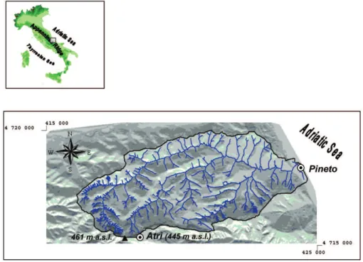
Fig. 1.Geographic location of the Calvano watershed. Projection East U.T.M. 33 European Datum 1950.
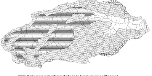
middle Pliocene-lower Pleistocene age (the Mutignano For-mation). The hilltops are constituted by sands and conglom-erates of marine-transitional and continental environments and capping clays with intercalated conglomerates and sands (“Blue Clays”, Fig. 2). Recent alluvial deposits and fluvial terraces (Holocene) are displaced along the valley bottoms.
The climate over the watershed is Mediterranean, with long dry summers and rainfalls concentrated in winter pe-riods. The average yearly rainfall is about 750 mm. The cli-matic regime induces soil aridity and superficial soil cracks during the summer, mainly on clay south facing slopes, which heavily affect slope stability and soil erosion vulner-ability. The soil is characterised by a reduced permeability that may induce flash floods after heavy rainstorms.
Land use is characterised by intense urbanisation along the coast and by scattered farms in the inner hilly areas, which are extensively cultivated with arables, olives and vineyards. The frequent use of cultivation techniques such as up and down tillage triggers rill/gully erosion and mudflow pro-cesses that, in turns, can generate severe erosion forms such as large mass movements and badlands on sandy-clay slopes. Nowadays, many cultivated areas are being abandoned and the natural vegetation is beginning to reinstate. Some small reservoirs are spread over the watershed for irrigation pur-poses.
According to Strahler’s classification, the Calvano River basin is ranked as 5th order. It shows a sub dendritic drainage network pattern, where the main stream is controlled by re-cent tectonic activity while secondary streams are strongly influenced by lithology and slope dynamics. In fact, the
hy-Table 1. Drainage density (Dd), hierarchical anomaly index (1a) and contributing area (A) for the watersheds considered by Ciccacci et al. (1987).
Watershed Dd 1a A
km−1 km2
Trebbia 0.23 0.08 226
Enza 0.25 0.05 670
Idice 0.25 0.06 397
Senio 0.18 0.06 269
Foglia 0.24 0.07 603
Orcia 0.22 0.07 580
Tavo 0.13 0.07 109
Volturno 0.16 0.08 2015
C. S. Maria 0.10 0.05 60
Triolo 0.13 0.06 54
Casanova 0.13 0.03 52
Salsola 0.13 0.05 43
Vulgano 0.11 0.07 94
Celone 0.14 0.05 86
Venosa 0.14 0.05 261
Atella 0.17 0.05 158
Agri (Grumento) 0.11 0.04 278 Agri (Tarangelo) 0.13 0.04 507
Delia 0.12 0.04 140
Gornalunga 0.19 0.05 232
Fig. 2.Geolithological scheme.
drographic network is mostly developed in the hilly part of the watershed, where well developed, sometimes spectacular, badlands systems (calanchi) occur, prevailingly on south fac-ing slopes. Both the main and the tributary watercourses are embedded in narrow valleys. The Calvano main stream val-ley opens in the coastal-alluvial plain which is rather limited in extensions as it is a few kilometres long from the conflu-ence of the two main tributaries (Fosso Reilla and Fosso di Casoli) to the sea mouth.
The above described geomorphological setting determines a significant risk of flooding for the human settlements lo-cated downvalley (CNR, 1993), mainly around the city of Pineto which is located on the river mouth. In July 1999 a severe flood occurred that submerged the coastal area with heavy damages to structures, roads, buildings and a high number of evacuees. Immediately after that catastrophic event, the local Authority commissioned a study with the aim to design precautionary measures and river engineering works to reduce the flood risk. The triggering factor of the flood that occurred in 1999 was recognised as the accumu-lation along the main stream of the Calvano River of sedi-ments supplied from the tributaries. The sediment yield was favoured by the low bedrock permeability, the high water-shed slope and the fine texture of sediments (Commissione Tecnica, 1999).
3 Framework of the analysis
The SSY is herein estimated by using the geomorphic ap-proach, depending on selected geomorphological features of the contributing watershed. For the Calvano watershed the
aim is to obtain a distributed picture of the concentration of suspended sediments along the river network, therefore iden-tifying the river reaches where sediment income and deposi-tion mainly occur.
The basic assumption of the method is that the SSY can be reliably predicted depending on the drainage densityDd
and the hierarchical anomaly index1aof the river network,
through a multiple regression approach that is calibrated by using an extended data set of SSY data collected in the 20 Italian river basins described in Sect. 2.1. We will identify withGathe minimum number of 1st order streams necessary
to make a drainage network perfectly ordered in a tree shaped structure with streams of orderuflowing into streams of or-deru+1. Then, the hierarchical anomaly index1ais given
by the ratioGa/N1(Avena et al., 1967), whereN1the
num-ber of 1st order channels actually occurring in the drainage network.
Ddand1aappear to be significant parameters when
esti-mating SSY, as they can synthesise the links among climatic, vegetation, river network and geological conditions whose combination results in watershed erodibility potential. From a mechanistic point of view, the connection among SSY,Dd
and1a can be explained by qualitative considerations. In
sedi-ments themselves, it follows that the link between SSY and drainage density should be non conservative with respect to an increase of watershed area. Therefore, if sediment depo-sition occurs, SSY and Dd should be non linearly related.
More specifically, under the assumptions that drainage den-sity decreases for increasing watershed area (because the av-erage slope of the watershed decreases as well) SSY should decrease more than linearly for decreasing drainage densi-ties.
An analogous reasoning may allow one to conclude that SSY should increase for increasing1a. In fact, a
hierar-chically anomalous river network implies that some streams flow into river reaches whose order is more than one unit greater. This induces an increase of SSY with respect to a perfectly ordered river network, given that the presence of anomalies typically indicates that the network is still under development and therefore the watershed is still undergoing a significant soil erosion. However, the structural form of the link between SSY and1a is not easily identifiable with a
qualitative analysis.
The recognition of the above links makes it reasonable to assume that a part of the variability of the SSY along the river network can be explained depending onDd and1a, with a
non linear relationship with respect to the former.
3.1 Estimating the suspended sediment yield through re-gression relationships
Ciccacci et al. (1987) developed an extensive analysis of SSY data that refer to the 20 Italian watersheds described in Sect. 2.1. They found a significant dependence among SSY, Ddand1athat is expressed through the following regression
equations:
SSY=100.33Dd+0.101a+1.45
(1) SSY=100.34Dd+1.52
(2) where SSY is expressed in Mg km−2year−1 and D
d in
km−1. Equation (2), whose independent variable isD
donly,
can be applied when1a is equal to zero, situation that
oc-curs in catchments only consisting of 1st order and 2nd order streams. In these conditions, hierarchic anomaly parameters have no significance, considering that anomaly arises when some streams flow into river reaches whose order is more than one unit higher. The independent variablesDdand1a
for Eqs. (1) and (2) above were estimated by analysing the drainage networks and basins contours mapped by using the 1:25 000 official topographic maps of the Italian Military Ge-ographic Institute (IGMI).
In a previous work, Ciccacci et al. (1980) observed that the exponential relationships above do not provide a good fit for highDd. Accordingly, they proposed to apply a bilogaritmic
relationships whenDdexceeds a threshold value. However,
in the present study the bilogaritmic approach was not con-sidered because of the lack of an extended experimental data
base that would be needed to perform a meaningful valida-tion of its results. Therefore Eqs. (1) and (2) were herein applied only to basins whereDd<7 km−1(with only one
ex-ception. See Sect. 4 for more details).
The form of relationships (1) and (2) agrees with the mech-anistic nature of the processes leading to SSY formation, in compliance with the qualitative considerations summarised above. Quantitative considerations to support the capability of the equations to reliably estimate SSY are provided here below.
3.2 Validation of the regression relationships
Ciccacci et al. (1987) reported a coefficient of determination for Eqs. (1) and (2) ranging from 0.95 to 0.96 and an av-erage percentage error of 14%. These statistics refer to the calibration mode and therefore provide limited information about the SSY estimates reliability in out of sample situa-tions. Therefore some considerations and further analysis are needed to substantiate the effectiveness of the above equa-tions when applied to ungauged basins. In fact, it is well known that regression approaches, as well as any empirical parametric model calibrated by fitting observed data, may ex-perience a decrease of performance when applied in practice. In order to inspect the capability of the proposed relation-ships to effectively predict the SSY in real world applica-tions a validation exercise was herein performed by applying a jack-knife technique (Haan, 1977). The main features of the validation procedure can be summarised as follows:
1. the attention is focused on the 20 watersheds where SSY,Ddand1adata are available;
2. one of these watersheds, say watershed s, is removed from the set;
3. the regression equations are recalibrated by considering the SSY data and geomorphic characteristics of the 19 remaining watersheds;
4. using the regression equations identified at step 3 above the SSY for watershed s is estimated;
5. steps 2–4 are repeated 19 times, each time with one of the remaining watersheds.
The 20 SSY estimates resulting from the model valida-tion, hereafter referred to as jack-knifed SSY values, are then compared with the corresponding observed SSY. The com-parison allows us to draw indications on the robustness and reliability of Eqs. (1) and (2).
0 500 1000 1500 2000 2500 3000
0 1000 2000 3000
Observed SSY [Mg km-2 year -1]
Predicted SSY [Mg km
-2 year -1 ]
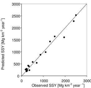
Fig. 3.Scatterplot of observed versus jack-knifed SSY values of the 20 Italian river basins studied by Ciccacci et al. (1987).
RMSE=97.6 Mg km−2year−1. The sample of errors that
af-fected the SSY estimates has a mean value that is not sig-nificantly different from 0 and a standard deviation equal to 116.38 Mg km−2year−1. Such errors look
homoscedas-tic with respect to the value of the SSY estimates (see Fig. 3) and the hypothesis of Gaussianity could not be rejected at the 95% confidence level accordingly to the Anderson-Darling and Kolmogorov-Smirnov normality tests (Kottegoda and Rosso, 1997). The above statistics could allow one to easily derive confidence bands for the obtained SSY estimates in real world applications. However, we believe that the sample of estimation errors is too short to allow a reliable uncertainty assessment. Nevertheless, it is evident that the performances of the proposed approach are satisfying for the purpose of obtaining a technically useful estimation of the suspended sediment yield along the river network.
3.3 Application of the regression relationships to ungauged watersheds
A first prerequisite for applying Eqs. (1) and (2) to ungauged catchments is to estimateDd and1a by using topographic
information with the same level of detail. Moreover, one should note that a decrease of the validation performances might be experienced if one applied Eqs. (1) and (2) to water-sheds that are not similar with respect to the ones that were considered in the jack-knife validation procedure. From a practical point of view, it is first of all necessary to check that the values ofDdand1aof the considered watershed do
not lie far too outside the range of the corresponding values of the calibration/validation data set. Table 1 shows theDd
and1a values of the watersheds considered by Ciccacci et
al. (1987), which were used to perform the validation above. The range of the testedDdand1avalues is also given in
or-der to provide technical indications about the applicability of the SSY estimation model. The homoscedasticity of the es-timation error with respect to the value of the SSY estimates (see Fig. 3) is a significant indication that the reliability of these latter should not abruptly decrease ifDd and1a
as-sume values that are slightly outside the ranges provided in Table 1. However, it is not advisable to sizeably extrapolate the regression equations.
Even ifDdand1aare compatible with the ranges spanned
by the calibration data set, one should take into account that the validity of the method was checked with respect to a rela-tively limited set of climatic, geologic and hydrologic condi-tions and a relatively limited range of watershed extensions (see Table 1). Therefore, any practical application should be preceded by a careful evaluation of the physical behaviours of the considered watershed, that should not be dissimilar with respect to those considered by Ciccacci et al. (1987). The main characteristics of these latter are given in Sect. 2.1. Further details can be obtained in Ciccacci et al. (1987).
Moreover, one should note that the proposed relationships provide an assessment of the annual average SSY. They are not conceived to provide an estimate of the SSY that may occur during a short time span when local events, like land-slides, may provide a significant contribution to SSY. Given that Eqs. (1) and (2) predict the SSY depending onDd and 1a, they are suited for case studies where the main
contri-bution to SSY comes from distributed soil erosion. This is the case of the 20 watersheds considered by Ciccacci et al. (1987) as well as the Calvano watershed. It follows that the role of spatially concentrated soil erosion should be care-fully considered and separately evaluated.
It is worth mentioning that the correlation between the SSY and the drainage density has proven to be not as sig-nificant in some cases (Grauso et al., 2007). For example, Cannarozzo and Ferro (1985, 1988) found drainage density to be poorly significant in predicting SSY for a number of watersheds located in Sicily (southern Italy). This outcome was attributed mainly to the climatic characteristics of the considered Sicilian basins, where the hydrological regime is characterised by highly variable discharges during the year, due to extended droughts in the summer followed by severe storms occurring in autumn and winter. This behaviour in-duces the presence of relevant soil erosion in autumn which is not correlated with the river discharge and therefore is poorly related to the behaviours of the river network (Grauso et al., 2007).
by Ciccacci et al. (1988). The SSY estimates were com-pared with reservoir sedimentation data and with estimates obtained by using different conceptual and empirical erosion models. The resulting differences were always lower than 10% (Ceci et al., 1998).
4 Application to the Calvano watershed
The regression Eqs. (1) and (2) have been herein applied to estimate the SSY for a series of subsequent river cross sec-tions of the Calvano watershed. Given that detailed infor-mation required to apply a physically based model are not available, the geomorphic approach appears to be a valuable opportunity for the sake of identifying the river reaches that are prone to sediment deposition. In fact, geomorphic param-eters can be estimated from maps or remote sensing observa-tions and can be downscaled to the desired spatial resolution. As it was mentioned before, an important requirement to assure the reliability of the above equations is to verify the similarity of the study watershed with the calibration and val-idation basins considered by Ciccacci et al. (1987). To this aim, the Calvano watershed can be included in this family of watersheds as it falls in the same geographic and mor-phostructural context and shows many similarities with re-gards to climate and geomorphological characteristics. Fur-thermore, it is important to note that the Calvano watershed is located few kilometres far from the Tavo River basin, which is one of the 20 fluvial basins considered by Ciccacci et al. (1987).
From a quantitative point of view, the 1a values of the
whole Calvano watershed and its subcatchments are all in-cluded in the respective range spanned by the calibration data set. The same is not true for theDd values. In order to
al-low an extensive application, Eqs. (1) and (2) were used up toDd<7 km−1, therefore allowing a 25% upper
extrapola-tion (see Table 1). In one case only a valueDd=7.51 km−1
was considered. The SSY estimates obtained for the sub-catchments where Eqs. (1) and (2) were extrapolated will be individually discussed when analysing the results.
Finally, a remark needs to be made about the watershed extension. In fact, the Calvano watershed is not included in the range of watershed size covered by the calibration data set. The extrapolation to small watershed sizes is much more significant for the case of the Calvano subcatchments con-sidered here (see Sect. 4.2). Figure 3 shows that the perfor-mances of Eqs. (1) and (2) are not significantly related to the watershed size, which varies in the range 43–2015 km2 for the watersheds tested with the jack-knife validation. There-fore we assume here that Eqs. (1) and (2) are still valid for predicting the SSY in river cross sections with a small con-tributing area (a few hectares). We are fully aware that this assumption may imply the presence of further uncertainty in the SSY evaluation, that could be reduced only by includ-ing in the calibration sample a number of additional small
basins. Therefore further research is needed to effectively support a technical application of the proposed approach to small size watersheds. We included such type of applica-tion in the present study in order to provide a first contribu-tion for addressing this concern, because the presence of hill reservoirs allows us to compare some of the derived SSY es-timates with reservoir siltation data. Although the latter too are affected by uncertainty that cannot be statistically quanti-fied, the comparison we carried out seems to confirm that the order of magnitude of the SSY estimates for the small size watersheds is consistent (see Sect. 4.3).
4.1 Quantitative geomorphic analysis and river network ac-quisition
The geomorphic parametersDd and 1a were obtained by
carrying out a quantitative geomorphic analysis of river net-work. This methodology makes it possible to obtain an ob-jective watershed characterisation and a quantitative compar-ison among different river basins (Horton, 1945; Strahler, 1957; Avena et al., 1967; Avena and Lupia Palmieri, 1969). The geomorphic parameters calculation was performed by means of the GIS tool Geomorf 2k5, which is the updated version of Geomorf 2k1 (De Bonis et al., 2002). Geo-morf 2k5 is an extension of ESRI ArcView®GIS 3.2a which adds to the user interface a set of tools for computing Strahler’s stream order and other geomorphic parameters. It also contains tools for removing several geometric and topo-logical inconsistencies in the river network layer induced by editing errors, mainly shape and connectivity errors such as pseudo nodes, overlapping arcs, under- or over-shootings, apparent connections with unsplitted arcs (Fattoruso, 2005).
The Geomorf 2k5 input data were the drainage network layer and the watershed layers. The permanent streams (blue lines) of the drainage network were mapped by using the 1:25 000 official topographic maps of the Italian Military Geographic Institute (IGMI). Additional information derived from the Regione Abruzzo maps with spatial scale of rep-resentation 1:10 000–1:25 000, aerial photographs and field observations were used to validate the blue lines. Moreover, a series of field surveys were carried out to check the con-sistency of the obtained blue lines with the current situation along the basin.
(a)
(b)
(c)
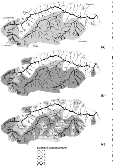
Fig. 4. Different patterns of the Calvano watershed subdivision: (a)4th orderpartial catchmentsdraining into the main stream;(b) previous plus 3rd ordersub- catchments;(c)previous plus 2nd and 1st ordersecondary catchmentsdraining into hill-reservoirs.
4.2 Basin subdivision
In order to evaluate the spatial distribution of soil erosion and sediment yield potential at different river sections, differ-ent subdivisions in minor order tributary basins were adopted (Fig. 4). The first subdivision groups the 4th order subcatch-ments (Table 2), to evaluate the gross sediment supply to the Calvano main stream. 4 subcatchments are identified (Cas-cianella, S. Patrizio, Reilla and Sabbione). The remaining main stream valley (5th order) is also treated as a subcatch-ment to investigate its sedisubcatch-ment supply potential.
The second subdivision is extended to the 3rd order sub-catchments. 17 subcatchments can be recognised, within the main stream and the 4 4th order subcatchments (Table 3). Another subdivision was performed by identifying the 1st
and 2nd order subcatchments which flow into small hill voirs (Table 4), in order to evaluate the contribution to reser-voir siltation.
A further subdivision was made in order to identify the 1st and 2nd order subcatchments affected by badlands (Fig. 5 and Table 5), with the aim to assess the relative significance of such severe erosion forms on the whole basin sediment balance.
4.3 Test catchments
Four test catchments were selected in order to verify the SSY estimates reliability on the basis of reservoir siltation data. These latter were obtained by means of bathymetric surveys and dredging operations that were carried out by the local ad-ministration and the owners. The information available about data collection do not allow derivation of an uncertainty en-velope for the reservoir siltation estimates. This is a frequent situation when dealing with such kind of information. How-ever, we believe that these data may provide a further confir-mation of the consistency of Eqs. (1) and (2) for small size watersheds.
Two test reservoirs are located within the Calvano River watershed. The first, named 20-Pineto, was built in 1959 and is located in the higher part of the Sabbione subcatch-ment. Its drainage area is 0.77 km2. The reservoir storage was assessed trough bathymetric surveys carried out by the local administration in 1974, when it was estimated to have a residual storage capacity of 30 000 m3instead of the initial 35 000 m3in 1959. Therefore, an average yearly sedimenta-tion rate of about 333 m3can be inferred, corresponding to a specific sediment supply of 4.3 m3ha−1year−1.
The second test reservoir, named 119-Atri, is located at the outlet of a 3rd order main stream tributary with a drainage area of 0.98 km2. It was built in 1970 with an initial storage capacity of 70 000 m3. After 35 years, a sediment volume of about 12 500 m3was estimated after a dredging operation, corresponding to a sedimentation rate of 357.14 m3year−1.
The other two test reservoirs, 147-Atri and 141-Atri, are located within two stream basins (Piomba and Cerrano streams) that are located very close to the Calvano water-shed and are characterised by very similar geomorpholog-ical behaviours. Both reservoirs have a contributing area of 0.15 km2. Sedimentation data were derived from
dredg-ing volumes. For the first reservoir, a sediment volume of 15 000 m3 was removed after 25 years, corresponding to a sedimentation rate of 600 m3year−1. For the second
reser-voir, a volume of 1600 m3was dredged after 22 years, corre-sponding to a sedimentation rate of about 70 m3year−1.
4.4 Results and discussion
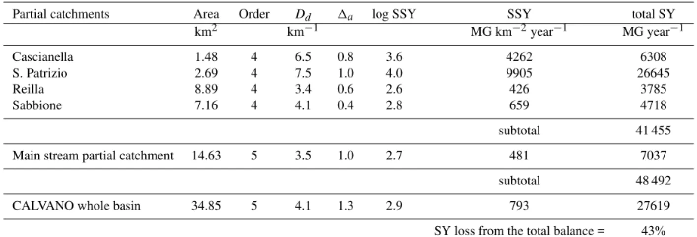
Table 2.Sediment yield estimates in 4th order subcatchments and the whole Calvano River basin.
Partial catchments Area Order Dd 1a log SSY SSY total SY
km2 km−1 MG km−2year−1 MG year−1
Cascianella 1.48 4 6.5 0.8 3.6 4262 6308
S. Patrizio 2.69 4 7.5 1.0 4.0 9905 26645
Reilla 8.89 4 3.4 0.6 2.6 426 3785
Sabbione 7.16 4 4.1 0.4 2.8 659 4718
subtotal 41 455
Main stream partial catchment 14.63 5 3.5 1.0 2.7 481 7037
subtotal 48 492
CALVANO whole basin 34.85 5 4.1 1.3 2.9 793 27619
SY loss from the total balance = 43%
Table 3.Sediment yield estimates in 3rd order subcatchments. SSY was not estimated whenDd>7.
Subcatchment Area Dd 1a log SSY SSY total SY
km2 km−1 MG km−2year−1 MG year−1
CASCIANELLA
sub13 1.07 6.6 0.6 3.7 4895 5223
sub12 0.12 11.2 0.5 – –
S. PATRIZIO
sub4 0.17 7.3 0.2 – –
sub5 0.20 7.3 0.4 – –
sub6 0.19 11.3 0.5 – –
sub7 0.44 5.7 0.0 3.4 2682 1180
sub11 0.09 7.5 0.0 – –
sub14 0.03 24.0 0.0 – –
REILLA
Vaccareccia 2.05 3.7 0.2 2.7 489 1002
sub8 0.68 4.3 0.0 3.0 933 635
sub15 4.92 3.4 0.5 2.6 395 1946
SABBIONE
sub9 1.05 4.5 0.0 3.0 1098 1153
sub10 1.15 4.9 0.4 3.1 1189 1368
sub16 4.77 3.8 0.4 2.7 551 2627
Main stream
sub1 0.33 6.1 0.3 3.5 3181 1050
sub2 0.70 4.0 0.3 2.8 612 428
sub3 0.98 2.7 0.1 2.3 220 215
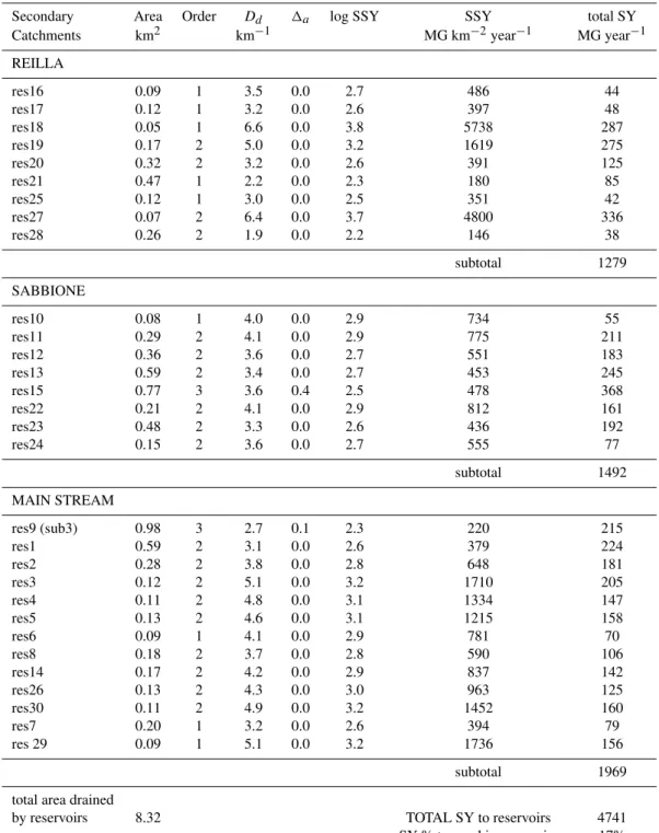
Table 4.Sediment yield estimates in secondary (mainly 1st and 2nd order) catchments draining into reservoirs.
Secondary Area Order Dd 1a log SSY SSY total SY
Catchments km2 km−1 MG km−2year−1 MG year−1
REILLA
res16 0.09 1 3.5 0.0 2.7 486 44
res17 0.12 1 3.2 0.0 2.6 397 48
res18 0.05 1 6.6 0.0 3.8 5738 287
res19 0.17 2 5.0 0.0 3.2 1619 275
res20 0.32 2 3.2 0.0 2.6 391 125
res21 0.47 1 2.2 0.0 2.3 180 85
res25 0.12 1 3.0 0.0 2.5 351 42
res27 0.07 2 6.4 0.0 3.7 4800 336
res28 0.26 2 1.9 0.0 2.2 146 38
subtotal 1279
SABBIONE
res10 0.08 1 4.0 0.0 2.9 734 55
res11 0.29 2 4.1 0.0 2.9 775 211
res12 0.36 2 3.6 0.0 2.7 551 183
res13 0.59 2 3.4 0.0 2.7 453 245
res15 0.77 3 3.6 0.4 2.5 478 368
res22 0.21 2 4.1 0.0 2.9 812 161
res23 0.48 2 3.3 0.0 2.6 436 192
res24 0.15 2 3.6 0.0 2.7 555 77
subtotal 1492
MAIN STREAM
res9 (sub3) 0.98 3 2.7 0.1 2.3 220 215
res1 0.59 2 3.1 0.0 2.6 379 224
res2 0.28 2 3.8 0.0 2.8 648 181
res3 0.12 2 5.1 0.0 3.2 1710 205
res4 0.11 2 4.8 0.0 3.1 1334 147
res5 0.13 2 4.6 0.0 3.1 1215 158
res6 0.09 1 4.1 0.0 2.9 781 70
res8 0.18 2 3.7 0.0 2.8 590 106
res14 0.17 2 4.2 0.0 2.9 837 142
res26 0.13 2 4.3 0.0 3.0 963 125
res30 0.11 2 4.9 0.0 3.2 1452 160
res7 0.20 1 3.2 0.0 2.6 394 79
res 29 0.09 1 5.1 0.0 3.2 1736 156
subtotal 1969
total area drained
by reservoirs 8.32 TOTAL SY to reservoirs 4741
SY % trapped in reservoirs 17%
and yearly total sediment yield SY (Mg year−1)are reported.
The specific sediment yield of the Calvano River was evalu-ated in 792.5 Mg km−2year−1, which is very close to the
av-erage observed SSY in river basins of central Italy (Abruzzo, Marche) flowing to the Adriatic Sea (see Lupia Palmieri, 1983).
The first level of basin subdivision (4th order) shows that the S. Patrizio stream can provide the highest sediment sup-ply within the whole basin (about 27 000 Mg year−1),
fol-lowed by the Cascianella stream (about 6000 Mg year−1).
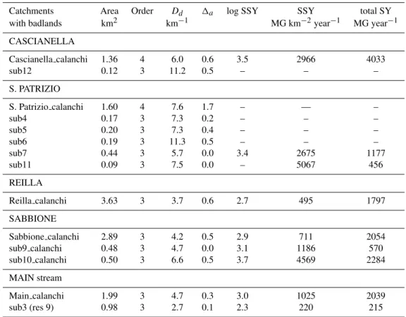
Table 5.Sediment yield estimates from catchments with badlands (calanchi). SSY was not estimated whenDd>7.
Catchments Area Order Dd 1a log SSY SSY total SY
with badlands km2 km−1 MG km−2year−1 MG year−1
CASCIANELLA
Cascianella calanchi 1.36 4 6.0 0.6 3.5 2966 4033
sub12 0.12 3 11.2 0.5 – – –
S. PATRIZIO
S. Patrizio calanchi 1.60 4 7.6 1.7 – — –
sub4 0.17 3 7.3 0.2 – – –
sub5 0.20 3 7.3 0.4 – – –
sub6 0.19 3 11.3 0.5 – – –
sub7 0.44 3 5.7 0.0 3.4 2675 1177
sub11 0.09 3 7.5 0.0 – 5067 456
REILLA
Reilla calanchi 3.63 3 3.7 0.6 2.7 495 1797
SABBIONE
Sabbione calanchi 2.89 3 4.2 0.5 2.9 711 2054
sub9 calanchi 0.48 3 4.7 0.0 3.1 1186 570
sub10 calanchi 0.50 3 6.6 0.5 3.7 4569 2284
MAIN stream
Main calanchi 1.99 3 4.7 0.3 3.0 1025 2039
sub3 (res 9) 0.98 3 2.7 0.1 2.3 220 215
Fig. 5.Location of catchments affected by badlands.
concluded that the river reach downstream their confluence is potentially critical in terms of sediment deposition. Anal-ogous situations would be identified if one evaluated the re-sults obtained at the second subdivision level (3rd order sub-catchments). One should note that theDdvalues of the
Cas-cianella and S. Patrizio watersheds are slightly outside the range spanned by the calibration data set. In particular, the S. Patrizio basin is the only exception where we applied the method forDd>7 km−1. Therefore the uncertainty of the
corresponding SSY estimates could be more significant with respect to what was inferred in Sect. 3.2.
It can be remarked that the sediment supply referred to the whole basin is lower than the sum of its subcatchment sediment yields. This is mainly explained by the different entity of drainage density. For example, when one refers to the entire Calvano basin (Dd=4.05 km−1), drainage density
is lower than the average Dd of its subcatchment (average Dd=4.99 km−1). This produces a sediment loss quantifiable
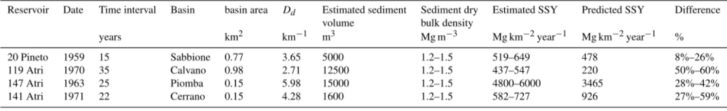
Table 6.Test-reservoirs sedimentation estimates and comparison with predicted SSYs by model equations. The dry sediment bulk density was allowed to vary in the 1.2–1.5 Mg m−3range.
Reservoir Date Time interval Basin basin area Dd Estimated sediment Sediment dry Estimated SSY Predicted SSY Difference
volume bulk density
years km2 km−1 m3 Mg m−3 Mg km−2year−1 Mg km−2year−1 %
20 Pineto 1959 15 Sabbione 0.77 3.65 5000 1.2–1.5 519–649 478 8%–26% 119 Atri 1970 35 Calvano 0.98 2.71 12500 1.2–1.5 437–547 220 50%–60% 147 Atri 1963 25 Piomba 0.15 5.98 15000 1.2–1.5 4800–6000 3465 28%–42% 141 Atri 1971 22 Cerrano 0.15 4.28 1600 1.2–1.5 582–727 926 27%–59%
average difference 38%
If one considered the 3rd order subcatchments of the Calvano River (Table 3), a mean SSY value of 1477 Mg km−2year−1would be estimated, but this value is
affected by the exclusion of the basins withDd>7 km−1that
will likely contribute with much higher SSY values. Table 4 reports the SSY estimates referred to river sec-tion located immediately upstream 30 small hill reservoirs located in the Calvano watershed. The overall area drained by reservoirs (8.32 km2)is about 24% of the whole Calvano basin. It turns out that 4741 Mg year−1of sediments are
en-tering into reservoirs. If one assumes that these sediments are completely trapped into the reservoirs, which is reasonable under appropriate working conditions, it appears that 17% of the Calvano yearly sediment yield might be trapped. This means that hill reservoirs are potentially effective in order to limit the siltation of the downstream river network.
Table 5 reports the SSY estimates obtained for the sub-catchments where the badlands (calanchi) are located. SSY was estimated only for those watersheds whereDd<7 km−1.
Badlands affect the whole area of Cascianella and S. Patrizio and a large portion of Reilla and Sabbione subcatchments. The total surface affected by badlands amounts to 14.64 km2, corresponding to 42% of the whole Calvano area. In general, the drainage density for all the badlands is significantly high, therefore implying that these areas are particularly prone to soil erosion. In fact, if one only considers the basins where Dd<7 km−1, their area is 35% of whole Calvano area, while
their SY is 44% of the total basin SY. By considering that the badlands with the higher drainage density (Dd>7 km−1),
and therefore the higher soil erosion potential, were excluded by this analysis, one can conclude that a significant part of the sediment supply to the Calvano main stream is produced by badlands. This is consistent with what is usually observed in environments with similar geomorphological behaviours.
SSY estimates were also computed for the small catch-ments draining into the selected test reservoirs. The com-parison between the sediment volumes trapped by the reser-voirs, converted into sediment yield, and the predicted SSY data allowed us to test the reliability of the SSY estimates for those small size basins (Table 6). The reservoir sediment volume data are to be converted into dry weight units and
corresponding specific sediment yield by estimating the dry bulk density of the sediments themselves. In absence of di-rect geotechnical measurements in the test reservoirs, we as-sumed that the dry sediment bulk density varies in the range 1.2–1.5 Mg m−3. This value was inferred on the basis of
di-rect measurements of humid sediment bulk densities rang-ing from 1.6 to 1.9 Mg m−3that were collected in the Penne
reservoir, located along the Tavo River (Ceci et al., 1998), which is similar to the Calvano River from a climatic and ge-omorphological point of view (the two watersheds are quite close each other, see Sect. 3.3 and Sect. 4). According to lit-erature indications, the above ranges and their interrelation are reasonable for low compaction sandy-clay materials.
Table 6 shows the range of the predicted SSY into the reservoirs, obtained by allowing the dry bulk density of the sediments to vary within the above range. It can be seen that in the four examined cases the predicted SSY show an average difference of 38% if they are compared with reser-voir sedimentation data, the best result being showed by 20-Pineto reservoir, where the difference between observed and predicted SSY is in the range 8%–26%. Reservoirs 119-Atri and 141-Atri show a more significant difference. Overall, it can be seen that the comparison provides consistent results. Even if the uncertainty that affects the sediment bulk density and the estimated SSY does not allow one to draw a final conclusion, the order of magnitude of the predicted values is consistent with what was estimated in the field. This result provides a first support to the assumption that the proposed method is valid for predicting the SSY in river sections with small contributing area (down to a few hectares).
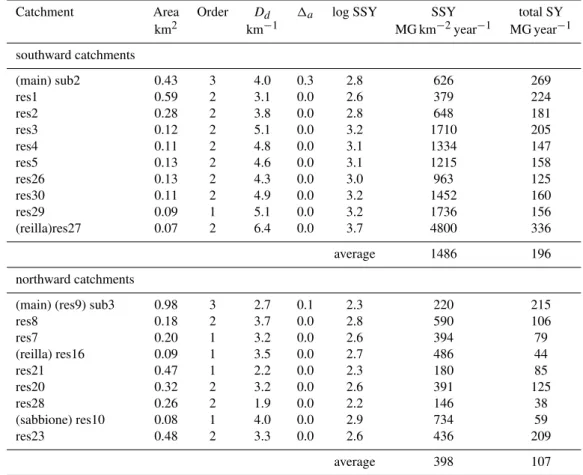
A last consideration concerns the relations between sedi-ment yield and basin exposure. In fact, if one grouped the examined secondary (mainly 1st and 2nd order) catchments into prevalently southward and prevalently northward facing (Table 7), one could see that the mean drainage density in the southward facing group is about 4.6 km−1, against a mean
value of 3.1 km−1for the northward facing group. The reason
Table 7.Sediment yield comparison between south- and northward facing catchments.
Catchment Area Order Dd 1a log SSY SSY total SY
km2 km−1 MG km−2year−1 MG year−1
southward catchments
(main) sub2 0.43 3 4.0 0.3 2.8 626 269
res1 0.59 2 3.1 0.0 2.6 379 224
res2 0.28 2 3.8 0.0 2.8 648 181
res3 0.12 2 5.1 0.0 3.2 1710 205
res4 0.11 2 4.8 0.0 3.1 1334 147
res5 0.13 2 4.6 0.0 3.1 1215 158
res26 0.13 2 4.3 0.0 3.0 963 125
res30 0.11 2 4.9 0.0 3.2 1452 160
res29 0.09 1 5.1 0.0 3.2 1736 156
(reilla)res27 0.07 2 6.4 0.0 3.7 4800 336
average 1486 196
northward catchments
(main) (res9) sub3 0.98 3 2.7 0.1 2.3 220 215
res8 0.18 2 3.7 0.0 2.8 590 106
res7 0.20 1 3.2 0.0 2.6 394 79
(reilla) res16 0.09 1 3.5 0.0 2.7 486 44
res21 0.47 1 2.2 0.0 2.3 180 85
res20 0.32 2 3.2 0.0 2.6 391 125
res28 0.26 2 1.9 0.0 2.2 146 38
(sabbione) res10 0.08 1 4.0 0.0 2.9 734 59
res23 0.48 2 3.3 0.0 2.6 436 209
average 398 107
that the estimated SSY from southward catchments resulted, on average, well higher than that from northward catchments.
5 Conclusions
This study considers the potential application of multiple re-gression relationships to estimate potential river sediment yield, depending on geomorphic parameters of the contribut-ing area. This kind of approach is potentially useful in order to obtain technical indications about sediment sources in a watershed in absence of the more detailed information that are needed in order to apply a physically based approach. Given that any empirical model, like the method considered here, is calibrated by referring to specific contexts and is po-tentially subjected to uncertainty in out of sample applica-tions, a jack-knife validation has been performed in order to test the performances of the suggested technique. Moreover, a further validation of the obtained sediment yield estimates has been performed by using reservoir siltation data.
By using simple regression relationships, such as those adopted here, it is possible to recognise the river cross sec-tions along the main stream which are more critical in terms of sediment yield and therefore the river streams were
sed-iment deposition is likely to occur. We believe this kind of approach might be a valuable opportunity for assessing the soil erosion potential over a watershed and stream siltation along a river network. However, the analysis herein carried out refers to a relatively limited range of drainage density and hierarchical anomaly index. Therefore, the analysis of addi-tional field data of suspended sediment yield is needed in order to widen the possible context of application of the pro-posed method. In particular, we believe additional research is needed to further test the reliability of the SSY estimates for small size watersheds.
Finally, one should note that the topological behaviours of the river network can be meaningfully related to the sus-pended sediment yield provided the soil erosion is signifi-cantly correlated with the river discharge. This requirement is not satisfied in the presence of local and massive sediment inputs to the river network, like those provided by landslides. This is an important consideration for practical applications.
Ungauged Basins (PUB) initiative of the International Association of Hydrological Sciences. The study has been partially supported by the Italian Government through its national grant to the pro-gram on “Advanced techniques for estimating the magnitude and forecasting extreme hydrological events, with uncertainty analysis”.
Edited by: S. Uhlenbrook
References
Agnesi, V., Del Monte, M., Fredi, P., Macaluso, T., and Messana, V.: Contributo dell’analisi geomorfica quantitativa alla valutazione dell’erosione del suolo nel bacino del fiume Imera settentri-onale (Sicilia centro-settentrisettentri-onale). Proceedings of the Work-shop “Erosione del Suolo, Gestione dei Sedimenti e Morfologia delle Coste”, Palermo, Italy, 101–115, 1996.
Anderson, H. W.: Relating Sediment Yield to Watershed Vari-ables, Transactions, American Geophysical Union, 38(6), 921– 924, 1957.
Avena, G. C. and Lupia Palmieri, E.: Analisi geomorfica quantita-tiva, in: Idrogeologia dell’alto bacino del Liri, edited by: Ac-cordi, B., Geologica Romana, VIII, Universit`a degli Studi di Roma, 319–378, 1969.
Avena, G. C., Giuliano, G., and Lupia Palmieri, E.: Sulla val-utazione quantitativa della gerarchizzazione ed evoluzione dei reticoli fluviali, Boll. Soc. Geol. It. 86, 781–796, 1967.
Battista, C., Boenzi, F., and Pennetta, L.: Una valutazione dell’erosione nel bacino idrografico del torrente Arcidiaconata in Basilicata, Suppl. Geogr. Fis. Dinam. Quat., 1, 235–246, 1988. Cannarozzo, M. and Ferro, V.: Un semplice modello regionale
per la valutazione del trasporto solido in sospensione nei corsi d’acqua siciliani, Atti Acc. Scienze Lettere e Arti di Palermo se-rie, V 5, 95–137, 1985.
Cannarozzo, M. and Ferro, V.: Confronto tra alcuni modelli per la previsione del volume di interrimento dei serbatoi artificiali siciliani. Atti Acc. Scienze Lettere e Arti di Palermo serie, V 8, 103–119, 1988.
Cavazza, S.: Contributo al calcolo del potenziale di erosione, Riv. It. Geof., 21, 27–32, 1972.
Cavazza, S.: Sulla erodibilit`a dei terreni di alcuni bacini calabro lucani, in: Aspetti geografici dell’erosione del suolo in Italia, edited by: G. Morandini, CNR Padova, 177–196, 1962. Ceci, D. P., Farroni, A., and Magaldi, D.: Applicazione del codice
di calcolo Raizal per la valutazione del rischio di erosione nel bacino del fiume Tavo, Geoingegneria Ambientale e Mineraria, Politecnico di Torino, 285–291, 1998.
Ciccacci, S., Fredi, P., and Lupia Palmieri, E.: Rapporti fra trasporto solido e parametri climatici e geomorfici in alcuni bacini idro-grafici italiani. Workshop “Misura del trasporto solido al fondo nei corsi d’acqua”, Consiglio Nazionale delle Ricerche, Flo-rence, Italy, 1977.
Ciccacci, S., Fredi, P., Lupia Palmieri, E., and Pugliese, F.: Contributo dell’analisi geomorfica quantitativa alla valutazione dell’entit`a dell’erosione nei bacini fluviali, Boll. Soc. Geol. It., 99, 455–516, 1980.
Ciccacci, S., Fredi, P., Lupia Palmieri, E., and Pugliese, F.: Indirect evaluation of erosion entity in drainage basins through geomor-phic, climatic and hydrological parameters, in: International
Ge-omorphology 1986 Part II, edited by: Gardiner, V., John Wiley and Sons Ltd, Chichester, 33–48, 1987.
Ciccacci, S., D’Alessandro, L., Fredi, P., and Lupia Palmieri, E.: Contributo dell’analisi geomorfica quantitativa allo studio dei processi di denudazione nel bacino idrografico del torrente Paglia, Suppl. Geogr. Fis. Dinam. Quat., 1, 171–188, 1988. CNR-GNDCI: Progetto AVI – Relazione Regione Abruzzo, U.O.
No. 10, Societ`a di Geologia Applicata, 1993.
Commissione Tecnica: “Progetto di massima e preliminare dei la-vori per l’eliminazione delle problematiche esistenti ed emerse a seguito degli aventi alluvionali del 9 e 10 luglio 1999”, Technical Report, Comune di Pineto, 1999.
De Bonis, P., Fattoruso, G., Grauso, S., Peloso, A., and Regina, P.: Computation of geomorphic parameters via GIS-based algo-rithms: a support tool in river systems management, Proc. Sec-ond International Conference “New Trends in Water and Envi-ronmental Engineering for Safety and Life: Eco-Compatible So-lutions for Aquatic Environments”, Capri, Italy, 136–137, 2002. Douglas, I.: Sediment sources and causes in the humid tropics of northeast Queensland, Australia, in: Geomorphology in a Trop-ical Environment, edited by: Harvey, A. M., Brit. Geom. Res. Group. Occ. Pap., 5, 27–39, 1968.
Fattoruso, G.: Hydrography and GIS’s – Removing Inconsistencies in Vector River Networks Extracted from Cartography, GeoIn-formatics, 8, 48–49, 2005.
Fournier, F.: Climat et ´erosion: la relation entre l’´erosion du sol par l’eau et les pr´ecipitations atmosph´eriques, Presses Univ. de France, Paris, 1960.
Gazzolo, T. and Bassi, G.: Relazione tra i fattori del processo di ablazione ed il trasporto solido in sospensione nei corsi d’acqua italiani, Min. lav. Pubbl., Giornale del Genio Civile, 6, 377–395, 1964.
Gazzolo, T. and Bassi, G.: Contributo allo studio del grado di erodi-bilit`a dei terreni costituenti i bacini montani dei corsi d’acqua italiani, Min. lav. Pubbl., Giornale del Genio Civile, 1, 9–19, 1961.
Grauso, S., De Bonis, P., Fattoruso, G., Onori, F., Pagano, A., Regina, P., and Tebano, C. : Relations between climatic-geomorphological parameters and suspended sediment yield in a Mediterranean semi-arid area (Sicily, southern Italy), Environ. Geol., doi:10.1007/s00254-007-0809-4, 2007.
Haan, C. T.: Statistical methods in hydrology, Iowa State University Press, 1977.
Horton, R. E.: Erosional development of streams and their drainage basins; hydrophysical approach to quantitative morphology, Bull. Geol. Soc. Amer. 56, 275–370, 1945.
Ichim, I. and Radoane M.: A multivariate statistical analysis of sed-iment yield and prediction in Romania, in: Geomorphological Models: Theoretical and Empirical Aspects, edited by: Ahnert, F., Catena Supplement, 10, 137–146, 1987.
Kirkby, M. J. and Cox, N. J.: A climatic index for soil erosion po-tential (CSEP) including seasonal and vegetation factors, Catena, 25, 333–352, 1995.
Kottegoda, N. T. and Rosso, R.: Probability, Statistics, and Relia-bility for Civil and Environmental Engineers, McGraw-Hill, New York, 1997.
Lor`e A. and Magaldi D.: Valutazione del rischio di erosione del suolo: un esempio in Provincia dell’Aquila, CNR Quaderni di Scienza del Suolo, 6, 5–18, 1995.
Lupia Palmieri, E., Ciccacci, S., Civitelli, G., Corda, L., D’Alessandro, L., Del Monte, M., Fredi, P., and Pugliese, F.: Geomorfologia quantitativa e morfodinamica del territorio abruzzese: il bacino idrografico del fiume Sinello, Geogr. Fis. e Dinam. Quatern., 18(1), 31–46, 1995.
Lupia Palmieri, E.: Il problema della valutazione dell’entit`a dell’erosione nei bacini fluviali, Proc. XXIII Congr. Geog. It. Catania, Italy, 143–176, 1983.
Massaro, M. E., Russo, M., and Zuppetta, A.: Analisi indiretta dell’entit`a dell’erosione nel bacino del fiume Tammaro, Geogr. Fis. Dinam. Quatern., 19(2), 381–394, 1996.
Renard, K. G., Foster, G. R., Weesies, G. A., McCool, D. K., and Yoder, D. C.: Predicting soil erosion by water. A guide to conser-vation planning with the Revised Universal Soil Loss Equation (RUSLE), United States Department of Agriculture, Agricul-tural Research Service (USDA-ARS) Handbook No. 703, United States Government Printing Office, Washington DC, 1997.
Restrepoa, J. D., Kjerfveb, B., Hermelina, M., and Restrepoa, J. C.: Factors controlling sediment yield in a major South American drainage basin: the Magdalena River, Colombia, J. Hydrol., 316, 213–232, 2006.
Strahler, A. N.: Quantitative Analysis of Watershed Geomorphol-ogy. Transactions, American Geophysical Union, 38(6), 913– 920, 1957.
Wicks, J. M. and Bathurst, J. C.: SHESED: a physically based, distributed erosion and sediment yield component for the SHE hydrological modelling system, J. Hydrol., 175, 213–238, 1996. Williams, J. R.: Sediment-yield prediction with universal equation using runoff energy factor, in: Present and prospective technol-ogy for predicting sediment yield and sources, ARS.S-40, U.S. Gov. Print. Office, Washington, 244–252, 1975.
Wischmeier, W. H. and Smith, D. D.: Predicting rainfall erosion losses from cropland east of the Rocky Mountains, United States Department of Agriculture – Handbook no. 282, United States Government Printing Office, Washington DC, 1965.