www.nat-hazards-earth-syst-sci.net/10/667/2010/ © Author(s) 2010. This work is distributed under the Creative Commons Attribution 3.0 License.
and Earth
System Sciences
First experience of seismodeformation monitoring of Baikal rift
zone (by the example of South-Baikal earthquake of 27 August 2008)
G. V. Vstovsky1and S. A. Bornyakov2
1All Russia Research and Design Institute of Atomic Machinery (Joint Stock Company “VNIIAM”), Moscow, Russia 2Institute of Earth’s Crust, Siberian Department of Russian Academy of Sciences, Irkutsk, Russia
Received: 11 November 2009 – Accepted: 19 March 2010 – Published: 7 April 2010
Abstract. A novel method of data processing – a structural functions curvature analysis method – was applied to the time series of seismodeformation monitoring of Baikal rift zone from April to November 2008, revealing the unique features of monitoring variable behaviour that can be considered as a revelation of precursors to the intensive South-Biakal earth-quake (M=6.3, at 09:31 on 27 August 2008). The idea of a new approach leans upon basic ideas of modern physics of self-organized criticality and open non-equilibrium systems in general.
1 Introduction
The advances in experimental seismology during the 70s and 80s of the last century had stimulated the development of instrumental works in geodynamic testing areas. Taking into account the deformation nature of earthquakes and the preceding geophysical phenomena, great attention had been paid to deformation monitoring. Its technical base had been improved step-by-step and this was a way from simple man-ually controlled mechanical constructions to complex tenso-metric laser and other automatic installations enabling us to obtain long-term deformation variable time series with re-quired discretization.
The development of a new synergetic concept of open systems evolution (Haken, 1983; Kondepudi and Prigogine, 1999) and its application to geological and seismological in-vestigations (Letnikov, 1992; Gol’din, 2005; Keilis-Borok, 1990; Bak, 1989; Sornette et al., 1989, 1995; Saleur et al., 1996; Heimpel, 1997; Bowman et al., 1998; Hainzl et al., 2000; Grasso et al., 1998; Zoller et al., 2002) made it possible
Correspondence to:G. V. Vstovsky ([email protected])
to develop an advanced methodology. It is aimed at disclos-ing and analysdisclos-ing the hierarchical structure of geophysical systems. One of many approaches of such a methodology is the analysis of correlation times (CT) of local processes in-vestigated by stochastic time series of geophysical variables. It is implied (Vstovsky, 2008) that, as the processes take place on/in the distributed self-organized system, the changes in the state of such a system must influence the course of the local processes. For instance, during the accumulation of deformation in the Earth’s crust under external and inter-nal factors, and as a consequence, the rearrangement of the crust space structure, CT of local deformation processes can change. The registration and adequate interpretation of such changes can be an effective tool for the monitoring of the states of both the separate regions and the lithosphere as a whole to reveal and forecast the transition and critical states in the lithosphere evolution process.
A structural functions curvature analysis method (SF-CAM) provides an effective tool for time series analysis (Vs-tovsky, 2008, 2006), enabling us to reveal the CT hierarchy on the basis of a simple quick operating mathematical appa-ratus.
In this work, the first experience of SFCAM application to the processing of seismo-deformation data on seismically active Baikal rift zone (BRZ) is described.
2 Monitoring location and technique
(a)
(b)
(c)
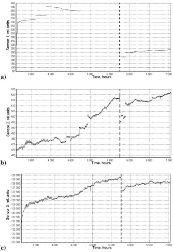
Fig. 1.Data of sensors 1, 2, 3 (a,b,c, respectively). Hour samplings are shown. Earthquake beginning is marked by dotted line.
Monitoring was carried out since April to November 2008. An intensive South-Biakal earthquake (M=6.3, at 09:31 on 27 August 2008) took place during monitoring time. Dur-ing this period, the automatic instrumental measurements of massive rock deformations were carried out in longitudinal, normal (with spreadings 150◦ and 60◦) and vertical direc-tions, sensors 1, 2, 3, respectively. The original bar sensors were used with a base 1.8 m and the ends fixed at the adit walls. Their active sensitive elements were beam type strain sensors by the “Scame” company. Sensors were placed at such marble regions that had no cracks. 30 s sensor sam-pling, digital data accumulation and storing was conducted by the “Sdvig” recorder (Ruzhich, 2004). The recorded sig-nals are shown in Fig. 1 as hour samplings. The time coor-dinate is given in hours from the beginning of the year. The earthquake beginning (5745.5 h) is marked by dotted line.
There were gapes in the data, due to technical reasons. The most significant gaps were in the data of (longitudinal) sensor 1 during the period just before the earthquake, so the results obtained by the data of sensors 2 and 3 were used to obtain the results discussed below.
3 Data processing method and results
The data were processed by the combination of SFCAM and sliding window method (SWM). The latter enables us to present dynamical variable series as a sequence of values of one or another parameter calculated for each position of a data window of a given length. The window time coordinate is a position of its forward boundary. For each window po-sition a structural function (SF) of orderpwas calculated by formula
8p(1)= 1 M
M
X
k=1
|h(tk)−h(tk+1)|p, (1) where h(t ) – signal value in the window of N samples (“points”), the signal being given discretely in points tk= k1t(1t – discretization step) along coordinatet,M=N− 1/1t,1– lag (argument) of SF equal to1t, 21t, 31t, . . . , (N8)1t,N8= (0.5–0.8)N,p– SF order.p=2 is used in the following and this index will be omitted. SF represents an effective tool in theoretical and experimental investigations of chaotic systems and processes, for example, in turbulence investigations (Frisch, 1995).
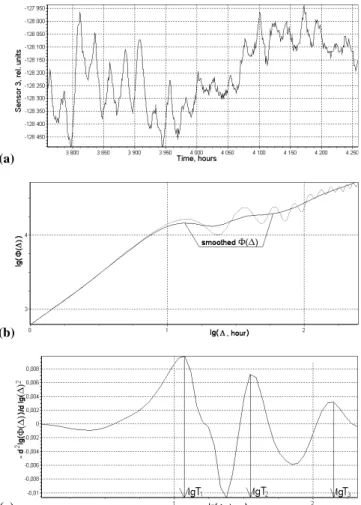
Figure 2 explains SFCAM. It shows examples of signal window, its SF (in double logarithmic axes) and the cor-responding negative second derivative of smoothed SF. Ex-tremuma positions of the latter give the evaluations of CTs.
The physical sense of SF is described here. The SF growth for small lags1 means that there are correlation links, in-terrelations, in the signal. The cessation of SF growth, sat-uration, for large lags means failure (lost) of the interrela-tions. The conventional boundary of these scale regions (de-termined by one or another rule or algorithm) is called a cor-relation time (CT). In the simplest cases, when SF has only one “footstep”, there is only one type of interrelation charac-terized by CT according to the “footstep position” which can be determined by the position of extremum negative deriva-tive of smoothed SF (under the condition of posideriva-tive first derivative) that was first proposed in (Vstovsky, 2006). That paper demonstrated the effectiveness of such an approach in comparison with many parameter fitness (approximation) of SF. When SF has several “footsteps”, corresponding to sev-eral interrelations with different CTs, the evaluation of SF’s negative second derivatives extremuma positions enables us to evaluate such CTs easily. Therefore, we can evaluate hier-archy of CTs. The case of SF with three “footstep” is shown in Fig. 2b and c. CTs are denoted byT1,T2,T3,. . . starting
with the smallest.
It should be stressed that the use of SF enables us, in this case, to reveal the presence of long term correlations with CT up to 1700 h (about 70 days) that corresponds to SF growth for lags larger than 1000 h. Such correlations witnessed con-cerning the strong non-stationarity of the processes under investigation and local instability of the lithosphere during the period before the disaster earthquake. The ability of the method to reveal such qualitative features of the system un-der study, shows in favour of the proposed approach.
The data were processed by a specially developed program called SHIFT (Scale Hierarchy Information Fertile Treat-ment), which enables the calculation of SFs, and their sec-ond derivatives, with the determination of CTs for any posi-tion of a window of given length and to calculate the depen-dence of the parameters on time. The used window size was 1000 samples (1000 h = 41.67 days). The window shift step was 20 samples. The maximum SF lag used here was 800 h (80% of window size).
Besides using SFCAM, the non-stationarity criteria were calculated to confirm the moments of significant changes in the system’s behaviour, registered by rearrangements of SFs and, consequently, by sharp changes of CTs. Let8k(1i) (1i=i∗1t )bei-th SF value calculated fork-th position of the sliding window. One non-stationarity criterion set pro-posed by Prof. Timashev (Descherevsky et al., 2003) (inte-gral relative criterion – IRC) reads
IRCk= P
i
8k(1i)−P i
8k−1(1i)
P
i
8k−1(1
i) ,
IRCk1=2
P
i
8k(1i)−P i
8k−1(1i)
P
i 8k(1
i)+P i
8k−1(1
i)
. (2a)
Another criterion set used in this work – relative integral cri-terion (RIC) – reads
IRCk=X i
8k(1i)−8k−1(1i) 8k−1(1
i) ,
IRCk1=2X i
8k(1i)−8k−1(1i) 8k(1
i)+8k−1(1i)
. (2a)
Values (2) must be approximately zero for stationary pro-cesses. Sharp changes of values (2), when window “slides” along the series, characterize the extent of non-stationarity of the processes under study. Criteria (2) can also be gener-alized for the use of other window functions such as power spectra, correlation functions, etc. instead of SF. But the ex-perience of their use showed effectiveness of criteria (2).
(a)
(b)
(c)
Fig. 2. SFCAM explanation. Window of sensor 3 signal(a), its double logarithmic SF and smoothed double logarithmic SF(b)and negative second derivative (“curvature”) of smoothed double loga-rithmic SF(c)with indication of extremuma positions which give CTs evaluations.
4 Results and discussion
Figure 3 shows the results of CTsT1,T2,T3calculation by
data of sensors 2 and 3 (the normal and vertical directions, respectively). As is seen, the sharp changes of CTs of lo-cal lithosphere deformation processes are observed approx-imately at 1200 h (by sensor 2 data) and at 800–1000 h (by sensor 3 data) before the earthquake. Such a behaviour wit-nesses the destruction of time correlations of the endogenic processes in the Earth crust that are due to the instability of the lithosphere space structure that results in significant re-arrangement of stress fields in the lithosphere and the prepa-ration of possible disaster rearrangement of the lithosphere structure, i.e. it results in an earthquake. Thus, we can say, in this case, about revelation of midterm (about 1100 h, 46 days) precursor of the disaster earthquake.
More exactly, a state with CTs T1=10 h, T2=30–40 h,
(a)
(b)
(c)
(d)
Fig. 3.Results of calculation CTsT1,T2(a, c)andT2,T3(b, d)by
sensors 2 (a, b) and 3 (c, d) data. Earthquake is marked by dotted line.
(both sensors), instable T2=5–20 h (sensor 2) andT2=10 h
(sensor 3), instableT3=20–50 h (sensor 2) andT3=40 h
(sen-sor 3) at 4800–5000 h, i.e. at 1000–800 h before the earth-quake. CTsT2,T3 of normal deformations (sensor 2) have
sharp oscillations in a wide range and reach great values T2=170 h,T3=365 h during such a transition. They also have
another wide range of oscillations at 300 h before the earth-quake. A state with T1=1–2 h, T2=6–8 h, T3=20–22 h for
both sensors takes place in 200 h after the earthquake. So, we can describe the registration of the system’s “switching” into another state. The decrease in all the CTs by 7–8 times
(a)
(b)
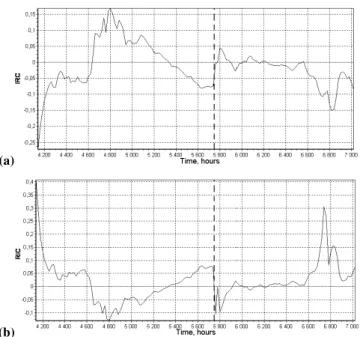
Fig. 4.The integral relative (IRC,a) and relative integral (RIC,b) non-stationarity criteria for sensor 3 data. IRC1and RIC1criteria
are almost the same in this case (but this is not true in general).
describes a strong rearrangement of the space structure of the system under study. At 7000 h, CTs become almost the same as at the beginning of observations after the transition through another instability for 6750–6900 h. It should be noted that CT’s changes just after a strong earthquake are hard to interpret as a precursor of the following events while the system is in an unstable state that can last for a year and longer.
The revealed moments of the system instability are con-firmed by the results of the calculations of non-stationarity criteria (2). Figure 4 shows the criteria for vertical deforma-tions (sensor 3) data. The registered moments of instability are almost the same – about 4800 h, very earthquake (5746 h) and about 6800 h.
BRZ represents an extended rift zone formed at the bound-ary of the Euroasia and Amur plates. High velocities of their relative movement (up to 10 mm/year and faster) provides the level of stresses in BRZ lithosphere, enough for the de-velopment of modern process of rift formation accompanied by high seismic activity.
As a rule, two, as a minimum, structural rearrangements forego the act of appearance of a single backbone break owing to the merging of multiple advance smaller failures (Seminsky, 2003). A universal feature, of the systems of ad-vance failures, is their ability to self-organization in the crit-ical state before structural rearrangements, resulting in rift dissipative structures (RDS) (Bornyakov et al., 2004, 2008). The characteristic features of their deformation processes are the coherence and autowave regime, i.e. the properties pe-culiar to lithosphere in metastable preseismogenic state, the properties reflecting the presence of cooperative phenomena (Gol’din, 2005; Keilis-Borok, 1990; Sobolev et al., 2003).
Following to general speculations above, it can be sup-posed that several months before the South-Baikal earth-quake the lithosphere in South Baikal region proceeded into a metastable state with formed RDS. The process of segmen-tation of the discontinuity flaw system, developing in RDS, is rather transient, runs in stages in reverse direction from the larger scales to the smaller ones (Bornyakov, 2008). Follow-ing the results obtained, approximately 1–1.5 months before South-Baikal earthquake, a process of self-organization and rearrangement of active segments network took place (ap-proximately 49 to 27 days before the earthquake). According to Sobolev et al. (2003); Sobolev (2008), the region of litho-sphere metastable state propagation can exceed the “nidus” region by an order and more, i.e. it can be hundreds of kilo-meters.
5 Conclusions
The results, obtained in this work, describe both the possi-bility of applying the proposed approach to disclose strong earthquake precursors and the rightfulness of seismic events analysis on the basis of general methodology of open sys-tems self-organization theory. The combination of perma-nent monitoring using the described tools and registration system with data processing on the basis of SFCAM and SWM can be considered for the perspective elaboration of an effective tool for preventive notification on the possible strong, seismic disaster events that can reduce the negative after-effects on responsible industrial and civil objects. The latter circumstance is of great importance now when there is an increase in seismic activity of the Earth’s crust during the last 10–15 years that compels us to reconsider the maps of seismic zoning.
Acknowledgements. The basic ideas of SFCAM were born after several years of dealing with a so called Flicker Noise Spectroscopy – a method of series processing which had been developed by Prof. S. F. Timashev. Authors thank Department of the Earth Sciences of RAS and Russian Fund of Basic Research for financial support of the field studies (Projects ONZ-7.7; RFBR 10-05-00678-a).
Edited by: M. E. Contadakis
Reviewed by: S. Sherman and another anonymous referee
References
Bak, P. and Tang, C.: Earthquake as a self-organized critical phe-nomenon, J. Stat. Phys., 54, 1441–1458, 1989.
Bak, P., Tang, C., and Winselfield, K.: Self-organized criticality, Phys. Rev. A, 38, 364–375, 1988.
Bornyakov, S. A., Cheremnykh, A. V., and Truskov, V. A.: Dis-sipative structures of rift zones and criteria of their diagnostics (by the results of physical modeling), Russ. Geol. Geophys.+, 49(N2), 179–187, 2008.
Bornyakov, S. A., Gladkov, A. S., Adamovich, A. N., Matrosov, V. A., and Klepikov, V. A.: Nonlinear dynamics of rift formation by the results of physical modeling, Geotechtonics, N5, 85–95, 2004.
Bowman, D., Ouillon, G., Sammis, C., Sornette, A., and Sornette, D.: An observational test of the critical earhquke concept, J. Geo-phys. Res., 103, 24359–24372, 1998.
Descherevsky, A. V., Lukk, A. A., Sidorin, A. Y., Vstovsky, G. V., and Timashev, S. F.: Flicker-noise spectroscopy in earthquake prediction research, Nat. Hazards Earth Syst. Sci., 3, 159–164, 2003
Frisch, U.: Turbulence. The Legacy of A. N. Kolmogorov, Cambtidge Univ. Press, 1995.
Gol’din, S. V.: Macro – and Mezostructures of focal earthquake re-gion, Physical mezomechanics, Novosibirsk, 8(N1), 5–14, 2005. Grasso, J.-R. and Sornette, D.: Testing self-organized criticality by induced seismisity, J. Geophys. Res., 103, 29965–29987, 1998. Hainzl, S., Zoller, G., and Kurths, J.: Seismic quinscence as an
indicator for large earthquakes in a system of self-organized crit-icality, Geophys. Res. Lett., 27, 597–600, 2000.
Haken, H.: Synergetics, an Introduction: Nonequilibrium Phase Transitions and Self-Organization in Physics, Chemistry, and Bi-ology, 3rd rev. enl. edn., Springer-Verlag, New York, 1983. Heimpel, M.: Critical behavior and the evolution of fault strength
during earthquake cycles, Nature, 338, 865–868, 1997.
Keilis-Borok, V. I.: The lithosphere as non-linear system with im-plications for earthquake prediction, Rev. Geophys., 28, 19–34, 1990.
Kondepudi, D. and Prigogine, I.: Modern thermodynamics: from heat engine to dissipative structure, 1999.
Letnikov, F. A.: Synergetics of Geological Systems, Novosibirsk, Nauka, 1992 (in Russian).
Ruzhich, V. V.: High-frequency measuring complex “Sdvig”. Sci-entific and industrial potential of Siberia: Investment projects, new technologies and elaborations, International catalogue, Novosibirsk, 90–91, 2004.
Saleur, H., Sammis, C., and Sornette, D.: Discrete scale invariance, complex fractal dimensions, and log-periodic fluctuations in seis-misity, J. Geophys. Res., 101, 17661–17667, 1996.
Seminsky, K. Zh.: Internal structure of continental rift zones: tectonophysical aspect, Novosibirsk, Siberian Dept. of RAS, 2003.
Sobolev, G. A., Lyubushin, A. A., and Zakrizhevskaya, N. A.: Asymmetric pulses, periodicity and synchronization of low-frequency micriseisms, J. Volcanol. Seismol.+, N2, 135–152, 2008.
Sobolev, G. A. and Ponomarev, A. V.: Earthquake physics and pre-cursors, Moscow, Nauka, 2003.
Sornette, D. and Sammis, C.: Complex critical exponents from renormalization theory group of earthquakes: Implication for earthquake prediction, J. Phys. I., 5, 607–619, 1995.
Vstovsky, G. V.: Revelation of spatial and temporal hierarchical structures in complex systems, in: Fluctuations and noise in com-plex systems of living and dead neture, edited by: Yul’metiev, R. M., Mokshin, A. V., Demin, S. A., Salakhov, M. Kh., Tatarstan Republic Ministry of Education and Science. Editorial and Pub-lishing Center “Shkola”, Kazan’ City, 441–454, 2008.
Vstovsky, G. V.: Factual Revelation of Correlation Lengths Hi-erarchy in Micro- and Nanostructures by Scanning Probe Mi-croscopy Data, Mater. Sci. (Kaunas), 12(3), 262–270, 2006. Zoller, G. and Hainzl, S.: A systematic spatiotemporal test of