A Convex Formulation for Magnetic Particle
Imaging X-Space Reconstruction
Justin J. Konkle1, Patrick W. Goodwill1, Daniel W. Hensley1, Ryan D. Orendorff1, Michael Lustig1,2, Steven M. Conolly1,2*
1Department of Bioengineering, University of California, Berkeley, CA, United States of America,
2Department of Electrical Engineering and Computer Sciences, University of California, Berkeley, CA, United States of America
Abstract
Magnetic Particle Imaging (MPI) is an emerging imaging modality with exceptional promise for clinical applications in rapid angiography, cell therapy tracking, cancer imaging, and inflammation imaging. Recent publications have demonstrated quantitativeMPIacross rat sized fields of view with x-space reconstruction methods. Critical to any medical imaging technology is the reliability and accuracy of image reconstruction. Because the average value of theMPIsignal is lost during direct-feedthrough signal filtering, MPIreconstruction algorithms must recover this zero-frequency value. Prior x-spaceMPIrecovery techniques were limited to 1Dapproaches which could introduce artifacts when reconstructing a 3D image. In this paper, we formulate x-space reconstruction as a 3Dconvex optimization prob-lem and apply robusta prioriknowledge of image smoothness and non-negativity to reduce non-physical banding and haze artifacts. We conclude with a discussion of the powerful extensibility of the presented formulation for future applications.
Introduction
Magnetic Particle Imaging is a novel, safe, sensitive, high-contrast, and fast imaging modality [1–6] with many potential applications in medical imaging including angiography, cell therapy tracking, cancer imaging, inflammation imaging, and temperature mapping [5,7,8]. TheMPI
technique detects only magnetic particles and derives no signal from tissue, which givesMPI
unique contrast that is best compared with tracer imaging modalities such as nuclear imaging. This is in contrast to Computed Tomography (CT) and Magnetic Resonance Imaging (MRI),
which are primarily anatomical imaging techniques. The physics and hardware required for
MPIare completely distinct from existing medical imaging modalities, andMPIimages cannot be
acquired usingMRIsystems.
MPIproduces images of magnetic nanoparticle (MNP) concentrations by detecting the
nonlin-ear magnetic response of anMNPdistribution to time varying magnetic fields. A strong static
magnetic field gradient or selection field saturates allMNPs in the field of view (FOV) except for a
region near the center of theFOVcalled a field-free region (FFR), which can be either a field-free
OPEN ACCESS
Citation:Konkle JJ, Goodwill PW, Hensley DW, Orendorff RD, Lustig M, Conolly SM (2015) A Convex Formulation for Magnetic Particle Imaging X-Space Reconstruction. PLoS ONE 10(10): e0140137. doi:10.1371/journal.pone.0140137
Editor:Joseph Najbauer, University of Pécs Medical School, HUNGARY
Received:April 4, 2015
Accepted:September 22, 2015 Published:October 23, 2015
Copyright:© 2015 Konkle et al. This is an open access article distributed under the terms of the
Creative Commons Attribution License, which permits unrestricted use, distribution, and reproduction in any medium, provided the original author and source are credited.
Data Availability Statement:All relevant data are available in the Supporting Information files, via Github (https://github.com/jjkonkle/mpiReconMatlab), and via Dryad (http://dx.doi.org/10.5061/dryad.cn58f).
Funding:This work was supported by the National Science Foundation Graduate Research Fellowship Program—DGE 1106400—http://www.nsfgrfp.org
(JJK), the California Institute of Regenerative Medicine—RT2-01893—https://www.cirm.ca.gov
point (FFP) or field-free line (FFL). A second low-frequency, time-varying (e.g., sinusoidal) homogeneous magnetic field called the drive field excites theMNPs. The drive field translates
theFFR, which causes a flip in magnetization when theFFRpasses over theMNPs. This flip in
magnetization induces a signal in a receive coil. TheFOVis extended using a slowly varying
focus field or shift field.
To reconstruct the received signal into an image, two distinct approaches to image recon-struction have been demonstrated: system function reconrecon-struction [1,2,9–15] and x-space reconstruction [3–5,16–19]. The system matrix method measures or simulates theMNP
response in a specificMPIsystem with a pre-defined trajectory to form a system matrix. The
sys-tem matrix is then used to reconstruct an image. In contrast, x-space methods use an image space continuity algorithm which do not require any simulation or pre-characterization mea-surements of theMNPresponse. However, current x-space continuity algorithms operate
sequentially on a single 1Dline at a time and do not take advantage of information along the
two perpendicular axes.
Optimization approaches have been used for image reconstruction inMRIandCTto increase
imaging speed, reduce image artifacts, and reduce dose [20–28]. For example, some techniques formulate theMRIandCTreconstruction process using reliablea prioriknowledge regarding the governing physics and imaging process such as smoothness, non-negativity, data consistency, sparsity, and multiple imaging channels [20,21,24,25].
These optimization approaches can be applied toMPI, where reliablea prioriinformation exists and can be used to improve reconstruction accuracy. In this paper we formulate theMPI
1D, 2D, and 3Dx-spaceDC(direct current or zero-frequency) recovery and image stitching
pro-cesses as a convex optimization for the first time while enforcing knowledge that the image must be both smooth and non-negative. This new optimization approach utilizes additional information along the two axes perpendicular to the excitation axis to improve on our previous x-space reconstruction.
Theory
The x-space systems theory forMPIis described in [3–5,16–18]. TheMPIsignal equation and
point spread function (PSF) were derived using the assumption thatMNPs instantaneously align
with an applied magnetic field [16,17]. The systems theory was then extended to include the first-harmonic direct-feedthrough filtering necessary in realMPIsystems [18]. The filtered
information was found to correspond to a loss of spatialDCinformation. X-space theory has
been used to prove analytically and experimentally that thisDCloss can be reversed to restore
linearity and shift invariance inMPI[18].
In this work, we demonstrate that theMPIx-space reconstruction process can be improved
in 2Dand 3Dusing convex optimization with the followinga prioriinformation: theMNP
distri-bution is non-negative and theMNPdistribution is smooth. The validity of these assumptions in MPIsystems is described below.
New a priori information: 2D
and 3D
smoothness and non-negativity
MPIimages the density ofMNPs convolved with a strictly positivePSF. Thus it is not possible for
theMPIimage, the convolution of two positive functions, to contain negative values except for
those produced by noise. Enforcing non-negativity during image reconstruction is then a phys-ically justifiable assumption.
The reconstructedMPIimage must also be smooth due to a smoothMPI PSF. The nativeMPI
image is a convolution of the physicalMNPdistribution with the smoothPSFand is thus smooth. 1R01EB013689—http://www.nibib.nih.gov(SMC), the
William M. Keck Foundation—034317—http://www. wmkeck.org(SMC), and the Sloan Research Fellowship—http://www.sloan.org(ML). The contents of this publication are solely the responsibility of the authors and do not necessarily represent the official views of the NIH, CIRM, UC Discovery or any other agency of the State of California. JK, DWH, PWG are employed/consult at Magnetic Insight, Inc. JJK, PWG, DWH, and SMC own stock in Magnetic Insight, Inc. The funders had no role in study design, data collection and analysis, decision to publish, or preparation of the manuscript.
If the sampling of the native image adheres to the Nyquist limit (determined by the band-lim-itedPSF), the reconstructed image must also be smooth.
In a multi-dimensional image reconstruction algorithm, one efficient method of incorporat-ing non-negativity and smoothness is through convex optimization methods, which can solve for convex objectives (e.g., the sum of a data consistency term and a 3Dsmoothness term) and
convex constraints such as non-negativity. The use of these additional terms and constraints enforces a globally optimal solution that adheres to the physics of theMPIprocess, thereby
increasing image conspicuity.
Materials and Methods
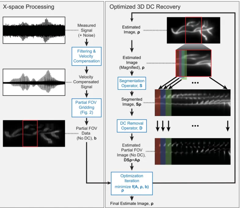
The reconstruction pipeline can be broken down into two serial processing steps: x-space pro-cessing and optimizedDCrecovery (seeFig 1). The x-space processing filters and velocity
com-pensates the raw data acquired by the analog to digital converters (ADCs) and interpolates the
data into partialFOVs. The optimizedDCrecovery then minimizes the residual error between
partialFOVdata and estimated partialFOVs. The estimated partialFOVs are calculated via a
for-ward operator on an estimated image. The linear operators that constitute the forfor-ward model are represented by sparse matrices and/or functions specific to a particularMPIpulse sequence.
The optimization problem includesa prioriinformation such as smoothness and non-negativ-ity. The problem is solved with a standard gradient descent-based algorithm using a matrix-free formulation which is fast, robust to noise, and memory efficient. We describe these steps in detail below.
X-space processing
X-space processing prepares the raw signal for the optimization problem and reduces the size of the dataset via three main steps: filtering, velocity compensation, and partialFOVgridding.
These steps remain identical to the previously reported x-space reconstruction and are illus-trated in the left column ofFig 1[16,18].
The filtering step of x-space processing recovers signal phase and reduces noise. Phase cor-rection filters reverse the phase distorted by the hardware filter chain. High pass filters remove any remaining direct-feedthrough at the fundamental frequency. Digital harmonic filtering removes signal outside a specified bandwidth of the received harmonics in the Fourier domain.
After filtering, velocity compensation is performed by normalizing the signal intensity to the instantaneousFFRvelocity as required for x-space reconstruction [16,17].
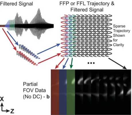
The signal is then gridded into partialFOVimages as detailed inFig 2. Image data is
interpo-lated onto a discrete grid using the known trajectory of theFFR. The trajectory is redundant and
creates overlapping partialFOVsub-images where one partialFOVis defined as the spatial extent
theFFRtravels due to the drive field. The resulting partialFOVdata is missing some unknown
portion of theDCcomponent in the partialFOVimage (along thez-axis inFig 2) due to direct feed-through filtering in hardware [10,18]. In this work, the remaining unknownDC
compo-nent is removed by filteringDCto zero.
Averaging during interpolation improves the final image signal to noise ratio (SNR) and also
reduces the storage size of the processed partialFOVdata when compared to the raw data
acquired by theADC. The original vector of raw data for the coronary phantom images shown
in this work contain 740 million values of data (6GB) while the partialFOVdata,b, contains 14
Linear Forward Model
A linear forward model describes the splitting of an image into partialFOVs and theDCsignal
loss due to filtering (seeFig 1, right side). The forward model is a simplified description of the imaging process. The linear forward model allows specification of the data consistency term of the optimization problem formulated inEq 6.
Fig 1. Experimental data illustrating proposed image reconstruction. (Left)The measured signal is filtered and velocity compensated before gridding to partialFOVimages. The partialFOV) images become the input to the optimization problem.(Right)The optimization problem formulation ofDCrecovery is
illustrated. The forward modelAconsists of theSandDoperators, whereSis the segmentation operator andDis theDCremoval operator. The initial estimated image is the zero vector,ρ0=0. The estimated image,ρ, is calculated and updated with each step of the iterative proximal gradient solver [29]. The
The forward model includes two operators, segmentationSandDCremovalD.Sis the
seg-mentation operator, which breaks the image into overlapping partialFOVimages:
S¼ Is
Ir
Is Is
Ir
Is
. . .
2
6 6 6 6 6 6 6 6 6 6 6 6 6 6 6 6 6 4
3
7 7 7 7 7 7 7 7 7 7 7 7 7 7 7 7 7 5
ð1Þ
whereIsis an identity matrix the size of the overlap,s, between adjacent partialFOVimages.Ir
is an identity matrix the size ofr=p−2swherepis the width of partialFOV. This definition is specific to the problem with the image vectorized along the rows and partialFOVs shifted by an
integer number of pixels.
Fig 2. Partial field of view gridding detail.The received signal is interpolated to partialFOVimages using the FFRtrajectory. Eachx-axis traversal is broken into a separate partialFOVimage. Varying colors delimit each
partialFOVimage. The sinusoidal pattern in the trajectory is formed due to the simultaneousx-axis shift field
The operator,D, removes the average along the drive field direction (here thez-axis) of the partialFOV:
D¼ R
R
. . .
R 2
6 6 6 6 6 4
3
7 7 7 7 7 5
ð2Þ
where
R¼Ip 1
p: ð3Þ
This operation is equivalent to subtracting theDCcomponent in the spatial Fourier domain.
OperatorsSandDare composed to form the forward model of theMPIsystem,A:
A¼DS ð4Þ
whereA2Rmn
is a matrix,nis the product of the dimensions of the resulting image, andm
is the product of the dimensions of the input partialFOVimages. Both operationsSandDare
sparse, and their composition results in anAmatrix that is sparse and has a block diagonal-like structure. The forward model is then described by:
b¼Aρ ð5Þ
whereb2Rmis the input data of vectorized partial
FOVs from the scanning system andρ2Rn
is the vectorized image ofMNPdensity convolved with the systemPSF. The vectors are built by
stacking the rows of the image or the rows of the partialFOV. Note that no assumptions
regard-ing nanoparticle behavior were made except that the nanoparticles respond to the instanta-neous position of theFFR.
Reconstruction Formulated as a Convex Optimization
Because we have represented the imaging process as a set of linear operations, we are able to estimate the nativeMPIimage by solving a convex optimization, expressed below. A convex
optimization formulation guarantees that any minimum reached is a global minimum [30].
minimize
ρ k
Aρ bk2
2 þakρk 2
2 þbi k reiρk
2 2
subject to ρ≽0 ð
6Þ
where≽denotes element-wise inequality for non-negativity,ρandbare as described inEq (5),
αis a Tikhonov regularization parameter,βiare smoothness parameters, andei,i2{1, 2, 3} is
one of the three coordinate axis basis vectors. The image non-negativity constraint improves the general robustness of theDCrecovery. As noted above, the addition of smoothness and
non-negativity terms are justified bya prioriknowledge of the physics.
The smoothness termsβi(which penalize the spatial image gradients) and the Tikhonov
regularizationαincrease the stability of the image reconstruction. Tikhonov regularization is used to better condition a problem. This is true of our problem as the Tikhonov term regular-izes the singular value associated withDC, originally in the nullspace, by forcing the
optimiza-tion to choose an image estimate with the lowest totalDCvalue. For our problem, this has a
Eq 3can be restated more generally:
minimize
ρ k
Tρ wk2 2
subject to ρ≽0
ð7Þ
where T¼ A ffiffiffi a p I ffiffiffiffi bi p rei 2 6 6 4 3 7 7 5 w¼ b 0 0 2 6 4 3 7
5 ð8Þ
In this form, the image reconstruction problem is a basic least squares problem subject to a non-negativity constraint. Many tools for solving this basic form of non-negative least squares are available in common scientific computing platforms; however, these tools do not support using matrix-free operators to solve optimization problems. Our motivation to use matrix-free methods is described in the next section. We implemented a proximal gradient algorithm (Fast Iterative Shrinkage-Thresholding Algorithm (FISTA)) using matrix-free operators, where the
proximal operator is a projection onto the non-negative orthant [29,31]. With this solver, we can compare the practical computational advantages and disadvantages of using matrix-free operator formulations over matrix formulations.
Linear Operator Representation
The image reconstruction problem can be complicated by the need to store very large matrices. Simply storing these matrices can be a challenge, even with considerable sparsity of approxi-mately 1:105. For example, the matrixAinEq 3requires approximately 32GB of memory for the 3Ddata sets acquired in this work when stored in a standard sparse form.
Instead of storing sparse matrices, matrix-free operators can be used. With matrix-free operators, the matrix-vector multiplication is encoded as a function, and no actual matrix is stored. These matrix-free operator methods are used inMRI,CT, and geology to reduce the
stor-age requirements of imaging problems [26,32,33].
In practice, there are two challenges in converting a given matrix formulation into the equivalent matrix-free operator formulation. First, one must derive a function for the forward linear map (Aρ). Then, to solve an optimization problem using this forward model, one must derive a function for the corresponding adjoint (A>b). Here, matrix-free operator formula-tions for both theDCremoval operator,D, and the splitting operator,S, and by composition,A,
were developed. The functional forms can be checked for correctness by operating on the iden-tity (returning the linear map in its finite, dense matrix form) and through the dot-product test [33]. As noted in the results section, going to matrix-free operator methods has improved reconstruction time seven-fold and greatly reducedRAMrequirements.
Imaging Phantoms
To demonstrate the reconstruction method using ourMPIsystem, two imaging phantoms were
created. A double-helix phantom shown inFig 3was fabricated from two 0.6mm inner diame-ter tubing segments injected withMNPs (Micromod Nanomag-MIP 78-00-102, Rostock,
Ger-many). These tubing segments were wound around a 2.7 cm acrylic cylinder with a total length of 6.5 cm.
A coronary artery phantom 3Dmodel with approximately human sized features was
cylindrical part. The part was printed on a 3Dprinter (Afinia H480, Chanhassen, MN). The 3D
model is shown inFig 4. The phantom was designed with 1.8mm by 2.3mm maximum diame-ter ardiame-teries that were approximately ellipsoidal. Injection holes (shown in black) had a diamediame-ter of 1.0mm and were filled with Micromod NanomagMIP MNPs diluted 4:1 with deionized water.
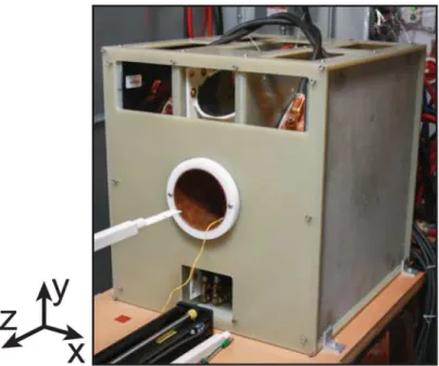
The phantoms were imaged with theFFPimaging system shown inFig 5. The images were
reconstructed using the formulation inFig 1. The optimization problem formulated inEq 4 was solved via a proximal gradient method developed in Matlab [29]. To reconstruct the image, 15 harmonics were used, for a total bandwidth of 300 kHz.
We included comparisons between native x-space reconstructed images and mildly decon-volved images in the results. Decondecon-volved images were generated using 3DWiener
deconvolu-tion [34]. The estimatedPSFreturned by blind deconvolution, seeded with a calculated
Fig 3. Experimental MPI data from a double helix phantom.The 3Ddataset was reconstructed using the previousDCrecovery method and the proposed
method. Both datasets are shown as maximum intensity projection images with no deconvolution. Images reconstructed with the proposed method contain less background haze and fewer artifacts. The imaging phantom was constructed by wrapping two 0.6mmIDtubes injected with Micromod NanomagMIP MNPs
around an acrylic cylinder ofOD2.7 cm. The total imaging time was 10 min with aFOVof 4.5 cm by 3.5 cm by 7.5 cm (x,y,z).
doi:10.1371/journal.pone.0140137.g003
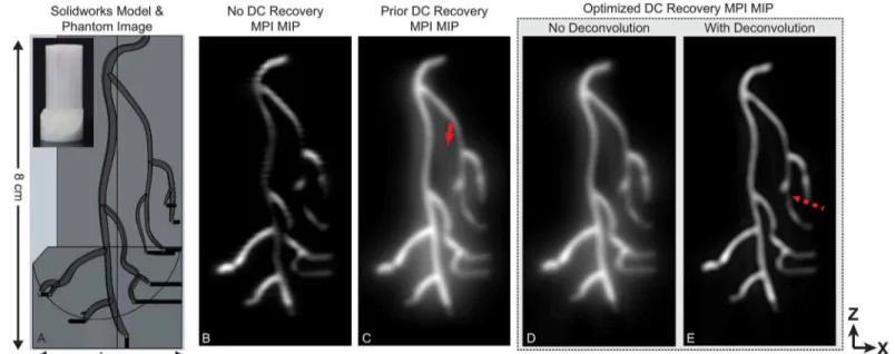
Fig 4. Experimental MPI data from a coronary artery phantom.Images were reconstructed with the proposed reconstruction formulation and contrasted to the previous 1D DCrecovery as well as noDCrecovery. The imaging phantom was created by 3Dprinting anABSplastic coronary artery model. The
reconstructed 3Ddataset is shown as maximum intensity projection images. With noDCrecovery, many image intensity dropouts are evident. These dropouts
are corrected withDCrecovery algorithms. The optimized 3Drecovery contains fewer artifacts (solid arrow) and less background haze than the prior
algorithm. Light deconvolution can be used to remove remaining background haze present in the reconstructed signal; however, deconvolution can lead to image dropouts (dashed arrow). The total imaging time was 10 min with aFOVof 4.5 cm by 3.5 cm by 9.5 cm (x,y,z).
theoreticalMPI PSF, was used in the Wiener deconvolution. Deconvolution was applied after
x-space reconstruction and independent of the optimization.
Results
InFig 3, the proposed reconstruction is compared to the previous x-space algorithm using experimentalMPIdata from a double helix phantom. Fewer banding artifacts and haze are
pres-ent with the proposed algorithm. No deconvolution is used. The 3Ddataset is further illustrated
in theS1 Video.
The following acquisition and reconstruction parameters were used for the images inFig 3: 46 partialFOVs, partialFOVmatrix size of 96 by 128 by 59 (x,y,z) pixels further downsampled
five-fold via averaging along thez-axis, 43.6 pixel overlap between partialFOVs,αof 0.15,βiof
0.048i, 10 iterations of theFISTAalgorithm, 96 by 128 by 154 (x,y,z) final pixel matrix size, total imaging time of 10 min, and aFOVof 4.5 cm by 3.5 cm by 7.5 cm (x,y,z).
InFig 4, the proposed reconstruction is contrasted with the case of noDCrecovery as well as
the previous x-space algorithm using experimentalMPIdata from a coronary artery phantom.
In the image with noDCrecovery, the partialFOVimages were averaged together to form the
image with no attempt to recover the lostDCinformation. There are obvious dropouts. When
deconvolution is used, the background haze in the image is reduced; however, deconvolution has introduced one image signal dropout (marked with a dashed arrow).
The imaging parameters forFig 4were: 46 partialFOVs, partialFOVmatrix size of 96 by 128
by 59 (x,y,z) pixels further downsampled six-fold via averaging along thez-axis, 43.6 pixel over-lap between partialFOVs,αof 0.05,βiof 0.048i, 30 iterations of theFISTAalgorithm, 96 by 128
by 129 (x,y,z) final pixel matrix size, total imaging time of 10 min, and aFOVof 4.5 cm by 3.5
cm by 9.5 cm (x,y,z).
Fig 6displays the data from the coronary artery phantom inFig 4with the proposed recon-struction at multiple angles of rotation to demonstrate the 3Dnature of the dataset. The 3Ddataset
is further illustrated in theS2 Video. The images are volume rendered views with deconvolution. Fig 5. Field free point MPI system photo.This 7Tm-1
FFP MPIsystem was used to experimentally
demonstrate the effectiveness of the 3Doptimized reconstruction.
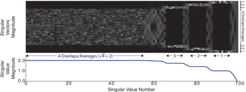
Fig 7shows the singular values and right-singular vectors of the singular value decomposi-tion (SVD) calculated for the operatorAto illustrate the conditioning of the proposed
recon-struction. The operator was created for a 1Dimage reconstruction to allow the singular vectors
to be shown easily. 15 pixels overlapped between adjacent partialFOVs and the partialFOV
width was 20 pixels. As expected, there is a singular value of zero for theDCimage component,
which indicates that an image with only aDCcomponent is in the nullspace of the operator. If
theDCsingular value is removed, the condition number of operatorAis 6.
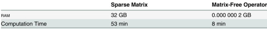
Table 1details reduced memory requirements using matrix-free operators when recon-structing the coronary phantom images ofFig 4. All reconstruction was performed on a single core of a computer with four Xeon 5600 processors and 144GBRAM. The conversion ofDto a
Fig 6. Experimental data of a coronary artery phantom fromFig 4at different angles.The 3D volume-rendered datasets were reconstructed using the proposed method with deconvolution. The total imaging time was 10 min with aFOVof 4.5 cm by 3.5 cm by 9.5 cm (x,y,z).
doi:10.1371/journal.pone.0140137.g006
Fig 7. Singular values and right singular vectors, V, were calculated on A for a 1Dproblem where 15 pixels overlapped between adjacent partial FOVs and the partialFOVwidth was 20.The singular vectors represent the spatialz-axis and are shown in absolute value. The singular values demonstrate
matrix-free operator reduced the reconstruction time 7-fold and reduced the storage require-ment of the operator to negligible amounts (2 × 10⁸fold reduction).
Discussion
For clinical acceptance of any medical imaging system, developers must produce a robust sys-tem that gracefully handles noise and minimizes image artifacts [35,36]. Here, we have designed an image reconstruction algorithm with these goals in mind.
InMPI, artifacts include banding and baseline drift. Banding artifacts manifest as ripples along
the horizontal and vertical axes due to discontinuities between partialFOVs. Haze occurs due to
the long tails of theMPI PSFand can be exacerbated by the reconstruction algorithm. Baseline drift
also appears as a hazy background, but this is likely due to component heating in theMPIsystem.
The proposed reconstruction formulation improves resulting image robustness and reme-dies many of the artifacts seen in prior x-space algorithms. For example, Figs3and4show that the proposed reconstruction has improved conspicuity and reduced artifacts, including sup-pressing banding and minimizing haze. Because of thea prioriinformation that the image is smooth, the banding artifacts do not occur in the images reconstructed via the optimization approach, which takes advantage of image smoothness along all image axes. The alpha term in the reconstruction optimization problem suppresses haze in the resulting images.
Reconstruction using the proposed formulation is well posed. The robustness of an optimi-zation problem can be seen in the magnitude of the operator matrix’s singular values. To illus-trate this, inFig 7we calculate the singular values and corresponding right singular vectors of a one-dimensional reconstruction using partialFOVoverlaps with similar properties as those
used in the full 3DAmatrix. We see that the singular value magnitude varies directly with the
amount of signal averages in a reconstructed image region; the singular value plateaus are equal to the square root of the number of partialFOVoverlaps. For example, for singular value
indices 1 to 64, each pixel in the central region is acquired four times in different partialFOVs
and these pixels have singular values ofpffiffiffi4¼2. Note the region of variation (marked with 4 averages along they-axis) in the singular vectors image corresponds to the section of four over-lapping partialFOVs where the singular value magnitude is 2.
The proposed algorithm can recover theDCinformation within a partialFOV, but there is no
a prioriinformation to recover the overallDCvalue of the image. This problem is common to
allMPItechniques that filter the signal direct-feedthrough. Note inFig 7that the right-most
sin-gular value of theSVDis zero; theDCvalue is in the null space ofA. The minimumDCvalue is
selected out of the null space by the optimization problem regularization term, which will be correctly selected if there is at least a single pixel value ofMNPconcentration within each line in
theFOV. Images taken withMPIare sparse and anatomical structures are tortuous by nature,
meaning images contain many zero values. Correct selection can be guaranteed by ensuring there is no tracer at one edge of theFOVduring scan prescription. Furthermore, even with this
condition not guaranteed, tests have indicated that the proposed algorithm still performs well. A reconstruction algorithm should not cause noise gain. As seen inFig 7, the 1D SVD
con-tains a small number of singular values less than 1. These singular values represent a noise gain Table 1. Sparse matrix versus matrix-free operator computation time and ram requirements.
Sparse Matrix Matrix-Free Operator
RAM 32 GB 0.000 000 2 GB
Computation Time 53 min 8 min
but the smoothness and Tikhonov terms suppress their noise amplification contributions. Fur-thermore, the very low frequency and straight line input distributions that would map to these singular values are not typically found in biological samples.
Beyond reconstruction,SVDanalysis can also be applied to the design ofMPIpulse sequences.
Inspection ofFig 7indicates that greaterSNRefficiency may be achieved by adding additional
acquisitions near the edge of theFOVto better condition the reconstruction. A larger drive field
will create more image overlap and thus more averaging but will not necessarily greatly improve the conditioning of the reconstruction. The same can be said about using a finer shift field pattern.
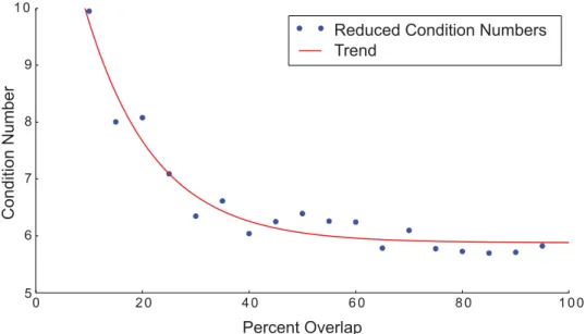
Reducing the overlap in the pulse sequence does not significantly increase the condition number until the overlap becomes small (seeFig 8). This indicates that reducing the overlap does not pose significant reconstruction problems until the overlap is only a small portion of the partialFOV. Though the conditioning does not significantly decrease, reduced averaging
due to reduced overlap will increase the noise seen in images as discussed above.
The aboveSVDanalysis demonstrates that image reconstruction via the proposed
optimiza-tion method is robust. Furthermore, the proposed method has been shown to produce fewer artifacts than the the previous x-space approach. We anticipate that improvedMPI
reconstruc-tion techniques such as optimized 3Dreconstruction will be crucial for the long term
accep-tance ofMPIin the clinic. In addition, we believe that these methods, along with advances in
hardware andMNPdesign, will be important for improved image quality in the future.
The proposed reconstruction technique contrasts with deconvolution, which if not used carefully and judiciously can degradeSNRand introduce artifacts such as signal dropouts. This
effect is seen inFig 4, where there is one dropout in the deconvolved image that is not present in the actual reconstructed image (marked with an arrow). However, deconvolution is able to reduce the haze present in the reconstructed image when applied minimally. It is thus vital that the benefits of deconvolution, such as reduction of haze, be balanced with the potential for introducing artifacts such as signal dropouts and ringing.
Fig 8. Condition number variation with overlap.The condition number is calculated on the matrixAwith theDCsingular vector removed (reducedA) for a 1Dproblem with a partialFOVwidth of 20. The trend curve is a
least-squares fit to the calculated condition numbers and illustrates the general trend of improved condition number with increased partialFOVoverlap.
The proposed reconstruction technique is fast and scales well. With matrix-free techniques, reconstruction occurs in eight minutes for the full 3Dvolume using only a single processor.
Moreover, many techniques could speed the solution of the optimization problem. Parallel pro-cessing techniques on multiple coreCPUs orGPUs could be used. Also, for real time imaging, a
prior reconstructed frame can be used to seed the optimization problem for rapid convergence. The proposed optimization approach is extensible in many ways. In general, newa priori
information can be incorporated into the reconstruction formulation. The proposed recon-struction can be modified for otherMPItrajectories, to add multiple simultaneous drive and
receive channels, and to include filtered backprojection forFFL MPIsystems. Expansion of the
formulation to include filtering and gridding steps of x-spaceMPIcan be explored. Relaxation
affects could be added to the formulation to improve reconstruction and enable new applica-tions. Compressed sensing approaches can be explored by reformulating the optimization problem and including objective terms such as sparsity transforms: wavelet transforms, dis-crete cosine transforms, or Chebyshev transforms. Many of these techniques have been used in
MRIandCTto improve image quality.
Conclusion
We reformulatedDCrecovery in x-space reconstruction as a 3Doptimization problem. This
represents the first implementation of x-space reconstruction to take advantage of information along axes perpendicular to the excitation axis duringDCrecovery on anFFP MPIsystem. The
reconstruction uses robust aa prioriinformation, non-negativity and image smoothness, to improve image quality. We applied the reconstruction algorithm to measured data and demon-strated improved robustness (less banding and haze artifacts) compared to our previous work. The framework developed here has improved flexibility over our prior 1D-at-a-time technique,
and shows promise for future work inMPI, including generalized trajectories in x-space,
projec-tion reconstrucprojec-tion, filtering incorporaprojec-tion, and compressed sensing.
Supporting Information
S1 Video. Experimental data of a double helix phantom.A video exported from OsiriX (Pix-meo SARL, Bernex, Switzerland) illustrates the 3Ddataset ofFig 3in rotated maximum
inten-sity projection. (MP4)
S2 Video. Experimental data of a coronary artery phantom.A video exported from OsiriX (Pixmeo SARL, Bernex, Switzerland) illustrates the 3Ddataset of Figs4and6in rotated
maxi-mum intensity projection. (MP4)
Acknowledgments
The authors would like to thank Kuan Lu, Bo Zheng, Elaine Yu, Nitish Padmanaban, Martin Uecker, and Jon Tamir for their helpful discussions and reviews of this work.
Author Contributions
References
1. Gleich B, Weizenecker J. Tomographic imaging using the nonlinear response of magnetic particles. Nature. 2005 Jun; 435(7046):1214–1217. doi:10.1038/nature03808PMID:15988521
2. Weizenecker J, Gleich B, Rahmer J, Dahnke H, Borgert J. Three-dimensional real-time in vivo mag-netic particle imaging. Physics in Medicine and Biology. 2009 Mar; 54(5):L1–L10. doi:
10.1088/0031-9155/54/5/L01PMID:19204385
3. Goodwill PW, Saritas EU, Croft LR, Kim TN, Krishnan KM, Schaffer DV, et al. X-spaceMPI: magnetic nanoparticles for safe medical imaging. Advanced Materials. 2012 Jul; 24(28):3870–3877. doi:10.
1002/adma.201200221PMID:22988557
4. Konkle JJ, Goodwill PW, Carrasco-Zevallos OM, Conolly SM. Projection reconstruction magnetic parti-cle imaging. IEEE Transactions on Medical Imaging. 2013 Feb; 32(2):338–347. doi:10.1109/TMI.2012.
2227121PMID:23193308
5. Saritas EU, Goodwill PW, Croft LR, Konkle JJ, Lu K, Zheng B, et al. Magnetic particle imaging (MPI) for NMR and MRI researchers. Journal of Magnetic Resonance. 2013 Apr; 229:116–126. doi:10.1016/j.
jmr.2012.11.029PMID:23305842
6. Saritas EU, Goodwill PW, Zhang GZ, Conolly SM. Magnetostimulation limits in magnetic particle imag-ing. IEEE Transactions on Medical Imagimag-ing. 2013 Sep; 32(9):1600–1610. doi:10.1109/TMI.2013.
2260764PMID:23649181
7. Weaver JB, Rauwerdink AM, Hansen EW. Magnetic nanoparticle temperature estimation. Medical Physics. 2009; 36(5):1822–1829. doi:10.1118/1.3106342PMID:19544801
8. Rahmer J, Antonelli A, Sfara C, Tiemann B, Gleich B, Magnani M, et al. Nanoparticle encapsulation in red blood cells enables blood-pool magnetic particle imaging hours after injection. Physics in Medicine and Biology. 2013 Jun; 58(12):3965–3977. doi:10.1088/0031-9155/58/12/3965PMID:23685712
9. Weizenecker J, Borgert J, Gleich B. A simulation study on the resolution and sensitivity of magnetic par-ticle imaging. Physics in Medicine and Biology. 2007 Nov; 52(21):6363–6374. doi:10.1088/0031-9155/
52/21/001PMID:17951848
10. Rahmer J, Weizenecker J, Gleich B, Borgert J. Signal encoding in magnetic particle imaging: properties of the system function. BMC Medical Imaging. 2009 Jan; 9(1):4. doi:10.1186/1471-2342-9-4PMID:
19335923
11. Knopp T, Rahmer J, Sattel TF, Biederer S, Weizenecker J, Gleich B, et al. Weighted iterative recon-struction for magnetic particle imaging. Physics in Medicine and Biology. 2010 Mar; 55(6):1577–1589.
doi:10.1088/0031-9155/55/6/003PMID:20164532
12. Knopp T, Biederer S, Sattel TF, Rahmer J, Weizenecker J, Gleich B, et al. 2D model-based reconstruc-tion for magnetic particle imaging. Medical Physics. 2010; 37(2):485–491. doi:10.1118/1.3271258
PMID:20229857
13. Lampe J, Bassoy C, Rahmer J, Weizenecker J, Voss H, Gleich B, et al. Fast reconstruction in magnetic particle imaging. Physics in Medicine and Biology. 2012 Feb; 57(4):1113–1134. doi:
10.1088/0031-9155/57/4/1113PMID:22297259
14. Rahmer J, Weizenecker J, Gleich B, Borgert J. Analysis of a 3-D system function measured for mag-netic particle imaging. IEEE Transactions on Medical Imaging. 2012 Jun; 31(6):1289–1299. doi:10.
1109/TMI.2012.2188639PMID:22361663
15. Knopp T, Weber A. Sparse reconstruction of the magnetic particle imaging system matrix. IEEE Trans-actions on Medical Imaging. 2013 Aug; 32(8):1473–1480. doi:10.1109/TMI.2013.2258029PMID:
23591480
16. Goodwill PW, Conolly SM. The x-space formulation of the magnetic particle imaging process: 1-D sig-nal, resolution, bandwidth,SNR,SAR, and magnetostimulation. IEEE Transactions on Medical Imaging. 2010 Nov; 29(11):1851–1859. doi:10.1109/TMI.2010.2052284PMID:20529726
17. Goodwill PW, Conolly SM. Multidimensional x-space magnetic particle imaging. IEEE Transactions on Medical Imaging. 2011 Sep; 30(9):1581–1590. doi:10.1109/TMI.2011.2125982PMID:21402508
18. Lu K, Goodwill PW, Saritas EU, Zheng B, Conolly SM. Linearity and shift invariance for quantitative magnetic particle imaging. IEEE Transactions on Medical Imaging. 2013 Sep; 32(9):1565–1575. doi:
10.1109/TMI.2013.2257177PMID:23568496
19. Konkle JJ, Goodwill PW, Saritas EU, Zheng B, Lu K, Conolly SM. Twenty-fold acceleration of 3D
projec-tion reconstrucprojec-tionMPI. Biomedizinische Technik Biomedical Engineering. 2013 Dec; 58(6):565–576.
doi:10.1515/bmt-2012-0062PMID:23940058
20. Lustig M, Donoho D, Pauly JM. Sparse MRI: The application of compressed sensing for rapid MR imag-ing. Magnetic Resonance in Medicine. 2007 Dec; 58(6):1182–1195. doi:10.1002/mrm.21391PMID:
21. Chen GH, Tang J, Leng S. Prior image constrained compressed sensing (PICCS): A method to accu-rately reconstruct dynamic CT images from highly undersampled projection data sets. Medical Physics. 2008; 35(2):660–663. doi:10.1118/1.2836423PMID:18383687
22. Block KT, Uecker M, Frahm J. Undersampled radial MRI with multiple coils. Iterative image reconstruc-tion using a total variareconstruc-tion constraint. Magnetic Resonance in Medicine. 2007 Jun; 57(6):1086–1098.
doi:10.1002/mrm.21236PMID:17534903
23. Griswold Ma, Jakob PM, Heidemann RM, Nittka M, Jellus V, Wang J, et al. Generalized autocalibrating partially parallel acquisitions (GRAPPA). Magnetic Resonance in Medicine. 2002 Jun; 47(6):1202–
1210. doi:10.1002/mrm.10171PMID:12111967
24. Uecker M, Lai P, Murphy MJ, Virtue P, Elad M, Pauly JM, et al. ESPIRiT-an eigenvalue approach to autocalibrating parallel MRI: Where SENSE meets GRAPPA. Magnetic Resonance in Medicine. 2014 Mar; 71(3):990–1001. doi:10.1002/mrm.24751PMID:23649942
25. Li M, Yang H, Kudo H. An accurate iterative reconstruction algorithm for sparse objects: application to 3Dblood vessel reconstruction from a limited number of projections. Physics in Medicine and Biology.
2002 Aug; 47(15):2599–2609. doi:10.1088/0031-9155/47/15/303PMID:12200927
26. Lustig M, Pauly JM. SPIRiT: Iterative self-consistent parallel imaging reconstruction from arbitrary k-space. Magnetic Resonance in Medicine. 2010 Aug; 64(2):457–471. doi:10.1002/mrm.22428PMID:
20665790
27. Tang J, Nett BE, Chen GH. Performance comparison between total variation (TV)-based compressed sensing and statistical iterative reconstruction algorithms. Physics in Medicine and Biology. 2009 Oct; 54(19):5781–5804. doi:10.1088/0031-9155/54/19/008PMID:19741274
28. Han X, Bian J, Eaker DR, Kline TL, Sidky EY, Ritman EL, et al. Algorithm-enabled low-dose micro-CT imaging. IEEE Transactions on Medical Imaging. 2011 Mar; 30(3):606–620. doi:10.1109/TMI.2010.
2089695PMID:20977983
29. Beck A, Teboulle M. A fast iterative shrinkage-thresholding algorithm for linear inverse problems. SIAM Journal on Imaging Sciences. 2009 Jan; 2(1):183–202. doi:10.1137/080716542
30. Boyd S, Vandenberghe L. Convex optimization. Cambridge University Press; 2004.
31. Parikh N. Proximal algorithms. Foundations and Trends in Optimization. 2014 Jan; 1(3):127–239. doi:
10.1561/2400000003
32. Man BD, Basu S. Distance-driven projection and backprojection in three dimensions. Physics in Medi-cine and Biology. 2004 Jun; 49(11):2463–2475. doi:10.1088/0031-9155/49/11/024PMID:15248590
33. Claerbout JF. Earth Soundings Analysis: Processing Versus Inversion. Cambridge, Massachusetts, USA: Blackwell Scientific Publications; 1992.
34. Gonzalez R, Woods R. Digital Image Processing. Third ed. New Jersey: Pearson Education, Inc; 2008.
35. Nienaber CA, von Kodolitsch Y, Nicolas V, Siglow V, Piepho A, Brockhoff C, et al. The diagnosis of tho-racic aortic dissection by noninvasive imaging procedures. The New England Journal of Medicine. 1993 Jan; 328(1):1–9. doi:10.1056/NEJM199301073280101PMID:8416265
36. Noone TC, Semelka RC, Chaney DM, Reinhold C. Abdominal imaging studies: comparison of diagnos-tic accuracies resulting from ultrasound, computed tomography, and magnediagnos-tic resonance imaging in the same individual. Magnetic Resonance Imaging. 2004 Jan; 22(1):19–24. doi:10.1016/j.mri.2003.01.