Dose assessment and reconstruction algorithm optimization in simultaneous breast and lung CT imaging

Bachelor of Science

Dose assessment and reconstruction algorithm

optimization in simultaneous breast and lung CT

imaging

Dissertation submitted in partial fulfillment of the requirements for the degree of

Master of Science in

Biomedical Engineering

Adviser: Phd. Salvatore Di Maria, Researcher, Centre for Nu-clear Sciences and Technologies - C2TN

Co-advisers: Phd. Nuno Miguel de Pinto Lobo e Matela, Associate Professor, Faculty of Science of University of Lisbon Phd. José Pedro Miragaia Trancoso Vaz, Main Re-searcher, Center for Nuclear Sciences and Technolo-gies - C2TN

Examination Committee

Chairperson: Phd. Carla Maria Quintão Pereira, Auxiliar Professor, FCT - UNL Raporteurs: Phd. Susana Evaristo Oliveira Branco, Adjunct Professor, ESTeSL

breast and lung CT imaging

Copyright © Débora de Souza António, Faculty of Sciences and Technology, NOVA Uni-versity of Lisbon.

The Faculty of Sciences and Technology and the NOVA University of Lisbon have the right, perpetual and without geographical boundaries, to file and publish this disserta-tion through printed copies reproduced on paper or on digital form, or by any other means known or that may be invented, and to disseminate through scientific reposito-ries and admit its copying and distribution for non-commercial, educational or research purposes, as long as credit is given to the author and editor.

First of all, I would like to express my profound gratitude to my adviser, Salvatore Di Maria and co-adviser, Nuno Matela, for their patience, dedication and efforts in bringing

this dissertation project to existence. Not only would this investigation not exist without them, but the synergy of their combined skills, expertise, and insights was crucial at every stage of the development of this project.

I would also like to express my sincere gratitude to my co-adviser José Pedro Trancoso Vaz and Octávia Monteiro Gil for their support and assistance both in a professional and personal level. To all the colleagues whom I encountered throughout my journey to accomplish this project, namely Mariana Baptista, Ana Belchior, Yuriy Romanets and Sandra Vieira, I am thankful for the assistance and time dedicated in providing me with crucial knowledge and advice of some software programs and equipment applied throughout the project. I would like to thank theC2T N, theIBEBand the Champalimaud

Clinical Centre, whose collaboration enabled me to undertake a dissertation project in a field of my personal preference and that I adore.

To my father, Fernando, my mother, Dalva, and my godmother Maria Alcine, who not only endured my many absences during the development of this project, but also provided me with their total support and encouragement, I offer my most heartfelt love,

appreciation and apology. I’m also profoundly grateful to my brother, Francisco, for his patience in listening to my daily problems, and for the laughs and pranks that would always make me smile. A great vote of appreciation goes to my aunt Ilda, and my uncle Mario, for their great support and thoughtful and encouraging words.

Cancer is the second leading cause of death in the world, and therefore, there is an undeniable need to ensure early screening and detection systems worldwide. The aim of this project is to study the feasibility of a Cone Beam Computed Tomography (CBCT) scanner for simultaneous breast and lung imaging. Additionally, the development of reconstruction algorithms and the study of their impact to the image quality was considered.

Monte Carlo (MC) simulations were performed using the PENELOPE code system. A MC geometry model of a CBCT scanner was implemented for energies of 30 keV and 80 keV for hypothetical scanning protocols. Microcalcifications were inserted into the breast and lung of the computational phantom (ICRP Adult Female Reference), used in the simulations for dose assessment and projection acquisition. Reconstructed images were analyzed in terms of the Contrast-to-Noise Ratio (CNR) and dose calculations were performed for two protocols, one with a normalization factor of 2 mGy in the breast and another with 5 mGy in the lungs. Both, MC geometry model and reconstruction algorithm were validated by means of on-field measurements and data acquisition in a clinical center. Dosimetric and imaging performances were evaluated through Quality Assurance phantoms (Computed Tomography Dose Index and Catphan, respectively).

Results indicate that the best implementation of the reconstruction algorithm was achieved with 80 keV, using theHanningfilter and linear interpolation. More specifically, for a spherical lung lesion with a radius of 7 mm a 30% CNR gain was found when the number of projections varied from 12 to 36 (corresponding to a dose increase of a factor of 3).

This research suggests the possibility of developing a CBCT modulated beam scanner for simultaneous breast and lung imaging while ensuring dose reduction. However fur-ther investigation regarding the number of projections needed for image reconstruction is required.

O cancro é a segunda principal causa de morte no mundo, e portanto, há uma ne-cessidade incontestável de garantir sistemas de rastreio e de diagnóstico precoce a nível mundial. Este projeto pretende estudar a viabilidade de um exame de Tomografia Com-putadorizada de Feixe em Cone (CBCT) na aquisição simultânea de imagens da mama e do pulmão.

Recorrendo ao sistema de código PENELOPE, realizaram-se simulações por métodos de Monte Carlo (MC). Implementou-se um modelo de geometria de um exame de CBCT, para energias de 30 keV e 80 keV, para possíveis protocolos de aquisição de imagem. Inseriram-se microcalcificações na mama e no pulmão do fantoma computacional (de Referência do ICRP) utilizado nas simulações, para avaliação de dose e aquisição de pro-jeções. Desenvolveram-se algoritmos de reconstrução e as imagens reconstruídas foram analisadas através da Razão Contraste-Ruído (CNR). Realizaram-se cálculos de dose para protocolos com fator de normalização de 2 mGy na mama e de 5 mGy no pulmão.

Tanto o modelo de geometria como o algoritmo de reconstrução, foram validados através de medições e aquisição de dados reais em ambiente clínico. Os desempenhos do-simétricos e de qualidade de imagem foram avaliados recorrendo a fantomas de Controlo de Qualidade (CTDI e Catphan, respetivamente).

Constatou-se que a melhor implementação do algoritmo de reconstrução foi alcançada com 80 keV. Nomeadamente, para uma lesão pulmonar esférica de raio 7 mm, alcançou-se um ganho de 30% de CNR variando o número de projeções de 12 para 36 (correspondendo ao aumento da dose de um fator de 3).

Este estudo sugere a possibilidade de se desenvolver um feixe modulado de CBCT para aquisição simultânea de imagens da mama e do pulmão, garantindo uma redução da dose administrada. É, contudo, necessária mais investigação relativamente ao número de projeções requeridas para a reconstrução da imagem.

List of Figures xvii

List of Tables xix

Acronyms xxi

1 Motivation 1

1.1 Cancer Incidence and Mortality . . . 1

1.2 Screening and Diagnostic Methods . . . 3

1.2.1 Breast Cancer . . . 3

1.2.2 Lung Cancer . . . 5

1.3 Purpose of the project . . . 6

2 Theoretical Concepts 7 2.1 Cone Beam Computed Tomography . . . 7

2.2 X-ray Radiation . . . 9

2.2.1 X-ray tubes . . . 11

2.2.2 X-ray spectrum . . . 12

2.2.3 Interaction of photons with matter . . . 17

2.2.4 X-ray linear and mass attenuation coeffi_{cients . . . . 20}

2.2.5 X-ray dosimetry . . . 23

2.3 Medical Image Reconstruction . . . 31

2.3.1 Radon Transform . . . 33

2.3.2 Backprojection . . . 35

2.3.3 Filtered Backprojection . . . 37

2.3.4 Inverse Radon Transform . . . 38

2.3.5 Image Quality . . . 40

3 Methodology 41 3.1 Monte Carlo Methods . . . 41

3.1.1 Geometrical Model Construction . . . 41

3.1.2 Monte Carlo Simulations . . . 43

3.2 Image Reconstruction . . . 49

3.2.1 From Projections to Reconstructed Images . . . 49

3.2.2 Image Quality Analysis . . . 51

3.2.3 Validation of the Reconstruction Algorithm . . . 51

4 Results and Discussion 55 4.1 CBCT Model Validation . . . 55

4.1.1 MC Simulations Validation . . . 55

4.1.2 Reconstruction Algorithm Validation . . . 57

4.2 Acquired Projections and Reconstructed Images . . . 58

4.3 Absorbed Dose Analysis . . . 60

4.4 Image Quality Analysis . . . 61

5 Conclusions and Future Work 67 References 71 A Detector Rotation and Source position and direction 77 A.1 Calculations of the Detector Rotation and Positioning . . . 77

B PenEasy files for performing the Monte Carlo Simulations 91 B.1 PenEasy.geo File . . . 91

B.2 PenEasy.in File . . . 94

B.3 Description for each entry of the penEasy.in File . . . 99

C PenEasy files for the PMMA Monte Carlo Simulations 105 C.1 The geometry file: PMMA.geo File . . . 105

C.2 The configuration file: PMMA.in File . . . 110

D Code system used in the Image Reconstruction milestone 117 D.1 Import data matrix . . . 117

D.2 Cube data matrix . . . 120

D.3 Division of the cube matrices . . . 120

D.4 Reconstruction Algorithm . . . 120

E Code system used in the validation of the reconstruction algorithm using Catphan 123 E.1 Import data matrix file . . . 123

E.2 Import data into cube data matrix . . . 123

E.3 Catphan Reconstruction Algorithm . . . 124

E.4 Catphan Algorithm for information acquisition . . . 124

1.1 World cancer incidence by sites. . . 2

1.2 World cancer incidence and mortality rates. . . 2

2.1 Fan Beam CT vs Cone Beam CT. . . 8

2.2 Arc-shaped detector vs Flat panel detector . . . 9

2.3 X-ray tube. . . 11

2.4 Anode focal point . . . 13

2.5 X-Ray spectrum . . . 13

2.6 An atom’s electronic shells . . . 14

2.7 Characteristic x-ray emission . . . 14

2.8 Bremsstrahlung emission . . . 15

2.9 Bremsstrahlung spectrum . . . 16

2.10 Compton scattering . . . 18

2.11 Mass attenuation coeffi_{cient in function of the x-ray energy . . . . 22}

2.12 Standard PMMA dosimetry phantoms . . . 28

2.13 ICRP adult male and female reference computational phantoms . . . 31

2.14 Reconstructed axial image: voxel and pixel . . . 32

2.15 Linear attenuation coeffi_{cient along the x-ray path . . . . 32}

2.16 Fan-beam geometry and parallel-beam geometry . . . 33

2.17 Projection data acquisition . . . 34

2.18 Sinogram . . . 35

2.19 Sinogram formation . . . 35

2.20 Discrete backprojection with interpolation . . . 36

2.21 Ram-Lak, block and triangle functions . . . 38

2.22 Ram-Lak,Shepp-Logan,CosineandHammingFilters . . . 39

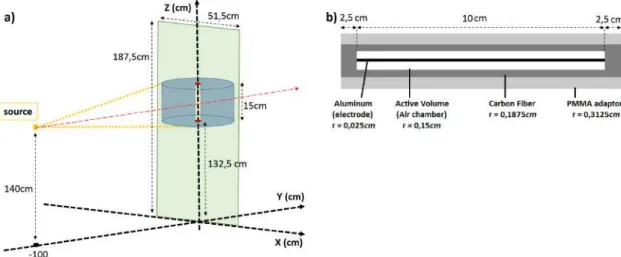
3.1 Geometry used for Monte Carlo simulations . . . 43

3.2 CT DI100simulated model and pencil ionization chamber configuration . . . 47

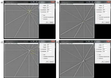
3.3 Gview2D: SimulatedCT DI100measurement model . . . 47

3.4 Cube data matix . . . 50

3.5 Breast and lung microcalcifications and background ROI’s . . . 52

3.6 Apparatus of the Varian TrueBeam with theCatphan 504. . . 52

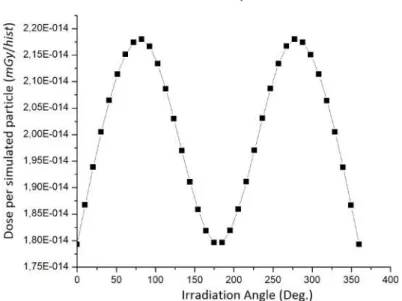
4.1 Graph of theCT DI100simulated values . . . 56

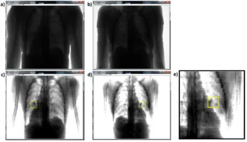
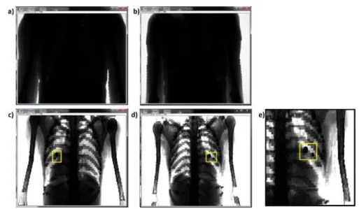
4.3 Microcalcifications within the projections obtained with 80 keV . . . 58

4.4 Microcalcifications within the projections obtained with 30 keV . . . 59

4.5 Reconstructed axial slice vs computational phantom axial slice using Gnuplot 59 4.6 Reconstructed axial slices using 30 keV . . . 60

4.7 Dose in breast and lung for diffrentent number os projections . . . 61

4.8 Graphs of the CNR for diff_{erent implementations: Breast . . . . 64}

4.9 Graphs of the CNR for different implementations: Lung . . . 64

A.1 Simplified schematic for detector rotation calculations . . . 77

A.2 Schematic of a 10° clockwise rotation of the detector . . . 78

A.3 The four quarters of the 360° rotation . . . 80

A.4 Schematic of the rotation when dealing with big angles . . . 80

A.5 Schematic of a rotation relativaly to the Original Coordinate System . . . 81

A.6 Schematic of the right triangles regarding the Origin . . . 81

2.1 Effective atomic number and relative densities of tissue, lipid and bone . . . 20

2.2 Tissue weighting factors,wT . . . 26

2.3 Filters and brief description . . . 39

3.1 Coordinates of the centers of mass of the organs of interest: Breats and Lungs 42 3.2 Coordnates of the centers of mass for each organ of interest and central point 42 3.3 Microcalcification Composition . . . 45

4.1 Air kerma experimental measurements . . . 55

4.2 CT DI100 experimental and reported measurements . . . 56

4.3 Air Kerma experimental and simulated values . . . 57

4.4 Reconstructed Images using Linear Interpolation . . . 62

4.5 Reconstructed Images using Cubic Interpolation . . . 63

A.1 Coordinates and angles of the point P1 for detector rotation . . . 84

A.2 Coordinates and angles of the point P2 for detector rotation . . . 85

A.3 Shift values for detector rotation . . . 86

A.4 Rectification of the shift values for both axis . . . 87

A.5 Source position . . . 88

A.6 Source direction . . . 89

I.1 Adult female reference computational phantom: elemental compositions of each organ/tissue . . . 126

ALARA As Low As Reasonably Achievable.

AP Antero-Posterior.

CBCT Cone Beam Computed Tomography.

CNR Contrast-to-Noise Ratio.

CP Central Point.

CRX Chest Radiography.

CT Computed Tomography.

CTDI Computed Tomography Dose Index.

DBT Digital Breast Tomosynthesis.

EM Electromagnetic.

FBP Filtered Backprojection.

FOV Field Of View.

FPD Flat Panel Detectors.

FT Fourier Transform.

ICRP International Commission on Radiological Protection.

ICRU International Commission on Radiation Units and Measurements.

IGRT Image-Guided Radiotherapy Technique.

LDCT Low-Dose Computed Tomography.

Linac Linear Accelerator.

MATLAB Matrix Laboratory.

MDCT Multi-detector Computed Tomography.

MRI Magnetic Resonance Imaging.

NLST National Lung Screening Trial.

PA Postero-Anterior.

PENELOPE PENetration and Energy Loss Of Positrons and Electrons.

PET Positron Emission Tomography.

PMMA Polymethyl Methacrylate.

ROI Region Of Interest.

SID Source-Isocentre-Distance.

C

h

a

p

t

e

1

M o t i va t i o n

1.1 Cancer Incidence and Mortality

Throughout the years, the number of diagnosed cases of cancer has grown at an alarm-ing rate. Cancer is the second leadalarm-ing cause of mortality worldwide with approximately 14 million new diagnosed cases, 8.2 million cases of cancer deaths and 32.6 million cases of people living with cancer in 2012 [1] [2]. One in six deaths worldwide, is due to cancer, [1] causing more deaths than AIDS, tuberculosis, and malaria combined [3]. It’s expected that by 2030, the global burden will grow to 21.7 million new cases of cancer and that can-cer deaths have reached 13 million cases [3]. According to the World Cancan-cer Report 2014, the three most commonly diagnosed cancers worldwide were lung cancer, accounting for 1.8 million cases (13.0% of the total globally diagnosed cases), breast cancer, accounting for 1.7 million cases (11.9% of the total globally diagnosed cases), and colorectum cancer, accounting for 1.3 million cases (9.7%), as shown in Figure 1.1.

Figure 1.1:Adapted illustration of a graphic of the estimated world cancer incidence proportions by major sites in both sexes, in 2012 [4].

Figure 1.2:Adapted illustration of a graphic of the estimated age-standardized cancer incidence and mortality rates (ASR) per 100 000 in the world, by major sites, in men and women in 2012 [4].

In some countries, among women, lung cancer mortality rate has surpassed breast cancer mortality rate, e.g., North America, Eastern Asia, Northern Europe, Australia and New Zealand [3].

1.2 Screening and Diagnostic Methods

In this section we will address screening and diagnostic methods that are currently recommended and implemented for lung and breast cancer. But first we will explain not only the main differences between screening and diagnosing a disease, but also the risks

and therefore the required cautions associated to each one. There are some screening and diagnostic methods that are still under development and/or have not yet been evaluated in assessing a mortality benefit, with randomized trials, and therefore, are not yet consid-ered a standard method for screening [7], consequently they will not be addressed in this chapter, e.g. autofluorescence bronchoscopy or exhaled breath analysis screening for lung cancer, and tomosynthesis screening for breast cancer [8]. Nevertheless, it’s important to refer that some may assess in the diagnosis, for instance the Digital Breast Tomosyn-thesis (DBT), which is steadily increasing in prevalence in hospitals and mammography facilities [9].

Cancer screening is a crucial tool, considering that the key to reducing cancer mor-tality relies strongly on an early detection and diagnosis [10]. Nevertheless, these are methods which asymptomatic, healthy patients are submitted to, with intend of an early diagnosis. The majority of screened patients are likely healthy and that otherwise would carry on with their lives normally if they hadn’t undergone screening, therefore the harms, risks and limitations associated to screening require crucial care and consideration in or-der to achieve balance between risk vs benefit [7] [11].

Contrary to imaging for screening, which asymptomatic patients are submitted to, a diagnostic evaluation is the process of assessing an existing problem or abnormality detected through screening [12]. Diagnostic imaging can be applied in two situations: a) imaging for clinical findings, i.e., if patient is manifesting symptoms that lead to cancer suspicion, as a palpable mass (in case of breast cancer) or persistent cough followed by sputum marked with blood (in case of lung cancer); b) incremental imaging after a possible abnormal screening exam [3] [12].

Although early detecting and diagnosing cancer is well known to be associated to a better prognosis and successful treatment, there are still many countries where late-stage diagnosis still occurs. This is mainly due to lack of awareness and to limited access to adequate detection and diagnostic services [3] [13].

Clinical guidelines on screening and diagnosing cancer, of all over the world, are constantly being developed, updated and reviewed, as new technological advances, new scientific investigations and new statistical data are taken in to consideration.

1.2.1 Breast Cancer

in women aged 50-69 years [9]. However, a recent guideline update from theAmerican Cancer Societyfor breast cancer screening, not only recommends that women should have the possibility to start annual screening mammography exams between ages of 40 and 44 years, and start with regular annual screening mammography exams from age 45 years, but also recommends that clinical breast examination should not be performed at any age [13]. As for theNational Comprehensive Cancer Network Breast Cancer Screening and Diagnosis Guidelines, they recommend an annual screening mammography beginning at the age of 40 [12]. Nevertheless, according to thePortuguese National Recommendations for diagnosis and treatment of breast cancer 09, the detection should be done through mammog-raphy exams, which still is the preferable screening method implemented in Portugal, or through prophylactic exams, e.g. Breast Self-Examination [14].

Mammography screening is basically a mechanism for breast imaging. Typically, it includes two x-ray images, being one taken from the top of the breast (craniocaudal), and the other taken from the side of the breast (mediolateral oblique) [12]. The Mammography Quality Standards Act limit is 3 mGy per view of screening mammography, for an average breast (5 cm thick and 50% glandular breast) [15]. Various studies have shown that mammography screening is associated to a reduction of breast cancer mortality, [13] however, it isn’t a perfect test.

The harms associated to mammography screening are mainly due to three factors: false-positive diagnosis, false-negative diagnosis and over diagnosis [11]. A false positive diagnosis is considered to be harmful, as it can lead to patient distress, and will result in unnecessary additional procedures, radiation exposures and/or biopsy [16]. False negative results are harmful, for obvious reasons, as it leads to breast cancers not being detected, delaying diagnosis and treatment [6] [17]. This occurs due to the inherent problem associated to the machine itself, which projects into a single plan the thickness of the breast, resulting in the overlap of tissue, which may obscure an abnormally, or even, lead to a false positive diagnosis [17]. Over diagnosing a cancer is when the disease is detected through screening however it wouldn’t lead to symptomatic breast cancer if it hadn’t been detected in the first place, and will lead to unnecessary therapy [6] [13].

As for diagnosing breast cancer, the procedure is basically based on clinical examina-tion, medical imaging and ultimately confirmed by pathological assessment [9]. However, this process involves a complex evaluation, and the procedures may differ from patient to

1.2.2 Lung Cancer

As previously seen, lung cancer is the leading cause of cancer death in developed countries, exceeding breast cancer death rate in women [3]. Frequently, this is due to the fact that screening for other cancer diseases is commonly practiced (e.g. breast, prostate, colorectum), whereas it is not for lung cancer [7].

The American College of Chest Physicians Guidelines, 3rdEdition, suggest annual screen-ing with Low-Dose Computed Tomography (LDCT), to people considered to be of high-risk, i.e., smokers or former smokers who are age 55 to 74 and who have smoked for 30 pack years (the number of packs of cigarettes smoked per day multiplied by the number of years a person has smoked) or more, and either continue smoking or have quitted within the past 15 years. Additionally they also state that screening should only be conducted in centers similar to those where the National Lung Screening Trial (NLST) was conducted, with coordinated care and complete knowledge of the screening process [7] [18]. NLST was the first randomized controlled trial which showed evidence of the benefits associ-ated to screening with LDCT in decreasing lung cancer mortality [19] [20].The American Society of Clinical Oncologistsalso state this same recommendation in their Guidelines: “The Role Of Computed Tomography Screening for Lung Cancer”[19].

Although lung cancer screening is not generally practiced worldwide, there is con-sensus in using LDCT technique as a screening method for individuals with high-risk factors.

LDCT is a computed tomography scan performed at low dose, using a tube voltage of 100-120 kVp and currents of 40-60 mAs or less [6]. The mean effective dose is 1.5 mSv for

LDCT, as for a standard Computed Tomography (CT), is 7 mSv, however when compared to a Chest Radiography (CRX), the dose delivered with a LDCT is greater (about 10 times greater) [17]. Alike mammography screening, LDCT screening also has risks inherent to it. The harms associated to LDCT are the same as described above in subsection 1.2.1 Breast Cancer, for mammography screening (false-positive results, false-negative results and over-diagnosis) [6].

1.3 Purpose of the project

C

h

a

p

t

e

2

T h e o r e t i c a l C o n c e p t s

In this chapter all theoretical concepts relevant for the comprehension of this project are explained. This chapter is divided into three main sections, in which the first one refers to the CBCT system, where a brief description of this mechanism and it’s main components, is made. The second section refers toX-ray Radiation and in this section all important concepts regarding x-ray radiation are described. It starts by describing the main concepts of particle collisions (e.g., Elastic and Inelastic collisions). In a second subsection, the instrumentation and x-ray production is described (X-ray tubes), followed by a subsection describing the x-ray spectrum and the physics underlying such radia-tion (Characteristic x-rays andBremsstrahlung). The fourth subsection approaches the Interactions of photons with matter, in whichRayleigh Scattering,Compton Scatteringand Photoelectric Effectare explained. This is followed by the subsection whereX-ray linear and mass attenuation coefficientsis referred to, in whichCross-sectionsare also explained. The last subsection isX-ray dosimetry, where three main sections are found:Measurements and units in photon dosimetry;Computed Tomography Dosimetry, where CT and CBCT dosime-try systems are referred to; andMonte Carlo Computation, where Monte Carlo simulations and voxelized phantoms will be addressed.

The last section, Medical Image Reconstruction, is a section in which not only the physics regarding data acquisition from CT scans are explained, but also some reconstruc-tion algorithms. This secreconstruc-tion is finalized withImage Qualityin which the measurement for analyzing the reconstructed images is described.

2.1 Cone Beam Computed Tomography

features, but always aiming for angiography purposes. It was only in the late 1900s, early new millennium, that CBCT systems started to emerge for dental and maxillofacial radi-ology purposes and for radiotherapy guidance (Image-Guided Radiotherapy Technique (IGRT)). Despite the CBCT concept not being a new discovery, it is an emerging tech-nology, and its use in clinical practices is gradually increasing. CBCT systems nowadays have a variety of medical applications that range from research to clinical applications. Ongoing studies are also being conducted to build a dedicated CBCT-based imaging sys-tem for mammography [23] [24] [25] [26]. For clinical applications it can be found, for example, for dental and maxillofacial imaging, head and neck imaging, high-resolution bone imaging (for orthopedic purposes), radiotherapy (IGRT), and intra-operative and interventional imaging (for angiographic CT). This strong rise in CBCT systems is due to recent technological advances, which made possible the development of clinical CBCT systems that are suffi_{ciently inexpensive and su}ffi_{ciently small to be used in operating}

rooms, clinics, intensive care units and emergency rooms [26].

A CBCT scanner is a subcategory of CT scanners, however it’s different from

Multi-detector Computed Tomography (MDCT) systems which are the industry standard for CT, with certain design features and application domains that are very specific and con-sequently the image quality differs from that of an MDCT. One of the most characteristic

feature of a CBCT system is the shape of its beam, which is in a cone shape rather than in a fan shape, as shown in Figure 2.1. The tomographic physics based on which CBCT operates, are basically the same as a MDCT [27] [26].

Figure 2.1:Adapted illustration of a fan beam CT scan on the left, and a cone beam CT scan on the right [28].

Another, very characteristic feature is it’s detector. CBCT scanners make use of Flat Panel Detectors (FPD), as shown in Figure 2.2, instead of an arc detector, as found in MDCT. The FPD system leads to a 2D bank of detectors which have no curvature, allow-ing higher spatial resolution and larger volume coverage in a sallow-ingle, or partial, rotation. However, this requires demanding reconstruction mathematics in order to apply correc-tion methods accounting for the different distances from source to detector [27] [26].

The gantry of a CBCT system differs depending on its applicability, hence the variety

Figure 2.2: Adapted illustration showing the diff_{erences between the arc-shaped detector used} in conventional CT systems on the left and the flat panel detector, used in CBCT systems, on the right [29].

c-arm-based CBCT, CT-gantry-based CBCT, co-integrated systems and CBCT in IGRT. In radiotherapy (IGRT), a CBCT system is used for precise alignment of the patient on the table of the Linear Accelerator (Linac) and there are two different modes, the kV

CBCT and the MV CBCT. The kV CBCT system is a separate system, consisting of an x-ray source, where the x-rays are produced using a conventional x-ray tube operating in the kV range, and a FPD. Both, x-ray tube and FPD come coupled to the Linac gantry, as they are mounted on retractable arms opposite to each other and positioned perpendicularly to the Linac’s beam. Despite the fact that a Linac gantry can only perform a 360° rotation, after which it must be rotated back, the CBCT system enables a large FOV to be imaged by scanning the target volume asymmetrically. This is accomplished by shifting the FPD laterally [27] [26] [30].

2.2 X-ray Radiation

X-rays are a type of Electromagnetic (EM) radiation that appears on the more energetic (smaller wavelength) end of the EM spectrum along with Gamma Rays, and their wave-length can range from 0.001 to 10 nm, corresponding to an energy range of approximately 0.052 to 129.544 keV [31].

This high energy EM radiation, not only exhibits wave-like behavior but also behaves as single particle-like "packets of energy"orquantaof energy, called photons. The energy of a photon is given by

E=hν=hc

λ (2.1)

where h is the Planck constant (h = 6.626×10−34 _{J.s = 4.136×10}−18 _{keV.s), ν is the}

frequency of the photon,cis the speed of light in vacuum (c= 2.998×108m/s≈3×108

m/s) andλis the photon’s wavelength [32].

For energy expressed in keV and the wavelength expressed in nm,h.c= 1.2397×10−6

eV.m, hence obtaining the following equation

E(keV) = 1.24

This is useful given that photon energies are usually expressed in electron volts (eV), which is a common unit of energy [27]. Electron volts is defined as the energy acquired by a single electron when submitted to an electrical potential difference of one volt, in

vacuum, this is 1 eV = 1.602×10−19_{J [33].}

Gamma rays are also photons and their energy range is usually of 100 to 10 000 keV. Despite the overlap of energies, x-rays and gamma rays are distinguishable by evaluating the photon’s origin. Therefore photon emissions that originate from the atom’s nucleus are identified as gamma rays, as for x-rays they have their origin in the rearrange of the atom’s electronic cloud or in the interaction of outer photons or particles with the the atom [34].

X-ray radiation is produced by x-ray tubes and it’s the outcome of the combination of two main interactions: bremsstrahlung and characteristic x-rays as we will see further on in section 2.2.2 X-ray Spectrum. Nevertheless we will first address certain concepts, as inelastic and elastic interactions as well as excitation and ionization, in the following section 2.2.0.1 Ionizing and non-ionizing interactions, as they are relevant concepts for further comprehension.

2.2.0.1 Ionizing and non-ionizing interactions

An inelastic collision occurs when a photon or any particle interacts with an atom and energy is transferred between the two, causing the ionization of the atom or leaving it in an exited state, in other words the interaction leads to a change in the atom’s internal structure and in the particles’ energy. Two examples of inelastic collisions are Ionization and Excitation. As for in an elastic scatter there’s no energy being transferred due to the interaction, only the particle’s trajectory is altered, in other words the particle is scattered but there’s no change to atom’s internal structure nor to the particle’s energy [35].

Ionization is the process by which one or more electrons are ejected from the atom or molecule as a result of the interaction with outer particles or photons. Excitation however, doesn’t imply the loss of electrons, but rather their transfer to a higher energy level, i.e., to an outer electron orbit, further from the atom’s nucleus, as a result of the interaction. Particles or photons with less energy are less likely to ionize an atom and will transfer their energy through excitation or elastic scattering which are processes that require less energy [36]. The minimum energy required to remove an electron, i.e., to ionize an atom is known as the ionization potential [37]. Charged and uncharged particles or photons that interact with an medium resulting in it’s ionization are considered Ionizing Radiation. Nevertheless, ionization and excitation are processes which cannot be separated, due to the fact that one given energy can result in the ionization of a given element but only lead to the excitation of another element. Therefore a pragmatic approach is usually used, in which a threshold for the energy (also known as a cutoff _{energy) is established. Below}

2.2.1 X-ray tubes

The device whereby the x-ray beam is generated and emitted is called the X-ray tube. It’s an equipment specialized to produce x-ray beams and it’s main components are typ-ically contained within an evacuated envelope made of Pyrex glass or metal [31]. The main components, this is, the minimum requirements for x-ray production are: an elec-tron source (cathode), an evacuated path for elecelec-tron acceleration (evacuated envelope), a target (anode), and an external power source (x-ray generator) supplying the power which provides a high potential difference for accelerating the electrons. In Figure 2.3 a

schematic of an x-ray tube’s main components is illustrated. The x-ray generator allows the selection of the three major parameters that determine the x-ray beam characteristics: the tube voltage (kV), the tube current (mA) and exposure time (s). Usually the product of the tube current and exposure time are considered as one entity, the milliampere-second (mAs) [27].

Figure 2.3: Adapted illustration of an x-ray tube with it’s major components: the evacuated envelope, which in the figure is represented as the x-ray tube insert, the cathode, the anode, the output port from where the beam is emitted and the circulating oil and lead shield which are essential to ensure the safety and effi_{ciency of the x-ray tube [27].}

The cathode is the source of electrons, consisting of a filament and a focusing cup. The filament is a spiral tungsten wire through which an electric current, up to 7000 mA and voltage of approximately 10 V, passes by. Heat is then generated through the resistance to electron flow through the filament, leading to a process in which the electrons of the filament’s material have sufficient energy and are released from it’s surface called

thermionic emission. By adjusting the filament current and consequently by the filament temperature, the number of electrons that are released can be controlled. The electron beam produced is emission-limited, this is, the filament current determines the x-ray tube current, meaning that the x-ray flux is proportional to the tube current, regardless of the tube voltage. However, it’s only when the potential diff_{erence (tube voltage) is applied}

between the cathode and the anode, within the evacuated envelope, that the released electrons flow [27] [38].

The tube voltage, this is, the electric potential diff_{erence, applied between the cathode}

and the anode, for diagnostic radiology purposes is of 20 to 150 kV. This potential diff

from the cathode to the anode they are accelerated due to the potential difference and

attain kinetic energy. This kinetic energy is equal to the product of the electrical charge and the potential difference. As previously mentioned, the electron volt (eV) is a unit of

energy which is equal to the energy acquired by an electron when accelerated through a potential difference of 1 V, therefore the kinetic energy of an electron accelerated by a

potential difference of 50 kV is 50 keV [27].

The target metal is called the anode, and it’s maintained at a large positive potential difference relative to the cathode in order to accelerate the electrons towards it. As

elec-trons interact with the anode their kinetic energy is converted into other forms of energy, like x-rays as mentioned before, but this only represents approximately 1% of the elec-tron’s energy, the majority is converted into thermal energy and therefore generating very high temperatures in the anode. To avoid heat damage the duration of x-ray production must be limited. Due to it’s high melting point of 3370℃ and high atomic number_Z=74,

tungsten is the most commonly used anode material. Nevertheless an anode rotor is at-tached to the anode which rotates at speeds of approximately 3000 rpm ensuring that the electron beam doesn’t strike the anode always at the same point and therefore reducing the localized heating. Additionally, within the tube housing, insulating circulating oil surrounding the whole envelope works as a cooling mechanism as shown in Figure 2.3 [27].

To guarantee a well defined small area in which the electrons will strike, the anode has a trapezium shape with an angle between 8° to 17° being 12° to 15° the usual range. Two of the major factor which are influenced by the anode angle are: the size of the focal point, the x-ray beam coverage and the x-ray beam intensity [38].

The focal point size (f) is given by:

f =Fsinθ (2.3)

whereF is the width of the electron beam andθis the anode’s angle, as shown in Figure

2.4. The focal point size range from 0.3 mm for digital mammography and 0.6 to 1.2 mm for planar radiography and CT. For small anode angles the focal point (f) becomes smaller for the same electron beam width (F), providing better spatial resolution.

There-fore the optimal anode angle depends on the clinical imaging application given that a small anode angle is preferable when dealing with a small FOV, which requires a smaller beam coverage, but for a large FOV, using a larger anode angle is more useful [38].

2.2.2 X-ray spectrum

Figure 2.4:Adapted illustration of the anode, showing the correlation between the electron beam widthF, the anode’s angleθand the focal point sizef [38].

Figure 2.5:Adapted illustration of an x-ray spectrum, showing the contributions of both interac-tions, bremsstrahlung and characteristic x-rays, to the produced x-ray beam [38].

characteristic X-rays) resulting in the production of x-rays with distinct energies that can be identified as distinct sharp lines in the plot of the energy spectrum, and through the interaction of electrons with the atomic nuclei causing their sudden deceleration (named Bremsstrahlung) resulting in the production of x-rays with an expanded spread of energies [32]. Both mechanisms will be discussed with greater detail in the following sections: 2.2.2.1Characteristic x-raysand 2.2.2.2Bremsstrahlung.

2.2.2.1 Characteristic x-rays

In the atom, each electron has a discrete energy state, according to the electron shell it occupies and each shell is denoted by a letter (K,L,M,N,...). The atom’s most inner shell is the K shell, for which the electrons have the lowest energy and therefore it’s the shell which requires the most energy to remove an electron from, as shown in Figure 2.6.

Figure 2.6:Adapted illustration of an atom’s electronic shells, their designations and the electron capacity per shell [27].

The interaction of outer electrons with an atom may result in the removal of an elec-tron creating a vacancy in one of the atom’s shell, and therefore, ionizing the atom. This is only possible if the energy transferred during their interaction is equal or greater than the atom’s orbital binding energy [27]. As a result, the atom is left in a very unstable state, for it will be lacking an electron in its electronic cloud, making it very unstable and therefore the vacant is rapidly filled by an electron from an outer shell. The transition of this electron between atomic shells will result in the emission of a single photon with energies in the x-ray range as shown in Figure 2.7.

Figure 2.7: Adapted illustration of the interaction that results in the emission of characteristic x-rays. The incident electron interacts with the K-shell electron, ejecting it. The created vacancy is rapidly filled with an outer electron that had to transit from it’s original shell and therefore emits energy, creating the characteristic x-rays [27].

The produced x-ray’s energy (Ex−ray) is given by the difference between the electron

binding energies (Eb) of both vacant shell and initial shell:

Ex−ray=Ebvacant−Ebinitial (2.4)

binding energies between the inner and outer shells involved in the process. Physicists call these kind of x-rays Characteristic X-rays and it can assume any energy typically from 0.052 to 129.544 keV. Given the fact that the atom’s shells only allow distinct energies, characteristic x-rays can only assume discrete energies [31] [27].

Characteristic x-rays are differentiated according to the shell where the vacancy is

located, for instance, when a vacancy in the K shell is filled, the resulting x-ray is called a K-characteristic x-ray. If the same vacancy is filled by an electron which transited from an adjacent shell, the x-ray is considered an alpha (e.g. an L to K transition will result in aKαcharacteristic x-ray). As for x-rays resulting from electrons which transited from

nonadjacent shells, they are considered beta (e.g. an M to K transition will result in the emission of aKβcharacteristic x-ray) [27].

2.2.2.2 Bremsstrahlung

Despite most electrons interacting with the atom’s electronic shell as they pass through matter, some undergo inelastic interactions with the atom’s nuclei. As a result of the in-teraction of these electrons with the positively charged nucleus, they suffer electrical

(Coulombic) forces of attraction causing a deflection in their path and resulting in a ki-netic energy loss which is instantaneously emitted as photons (i.e., x-rays). The kiki-netic energy lost by the electrons are equal to the energy of the radiation emitted and therefore energy is conserved. Due to this association between the electron deceleration and the photon emission, this process of x-ray production is called Bremsstrahlung which means ’brake radiation’ in German [37] [27].

Figure 2.8: Adapted illustration of the diff_{erent x-ray energies that may be produced through} bremsstrahlung, regarding the diff_{erent distances for which the incident electrons (1,2 and 3)} approach the atom’s nucleus [27].

producing higher x-ray energies, as shown in Figure 2.8. The highest x-ray energies are produced when the electron and atomic nuclei are the closest (or when impact occurs), however these close interaction has a very low probability of occurring and therefore the number of high energetic photons produced is very low. [27].

The produced x-rays can have energies that range from zero up to, and including, the entire energy the deflected electron had, originating a continuous spectrum that will cover that same range of energies. Usually the bremsstrahlung spectrum is filtered, this is, there’s a removal of the less energetic x-rays when the beam goes through ma-terials which are inherent to the x-ray tube (e.g., the tube’s glass window) or through purposefully placed materials in order to adjust the spectrum to the wanted energies (e.g., aluminum or copper sheets) [27]. A bremsstrahlung spectrum can be seen as the probability distribution of x-ray photons as a function of the energies for those same photons as shown in Figure 2.9, where the highest x-ray energy is determined by the peak voltage (kVp), as mentioned in section 2.2.1X-ray tubes[37] [27].

Figure 2.9: Adapted illustration of a filtered bremsstrahlung spectrum plot, for a 90kVp opera-tional voltage [27].

The probability of bremsstrahlung emission is proportional to the atomic number of the absorber, which is given by the valueZ2but it is inversely proportional to the square of the mass of the incident particle, this is, Z2/m2. Therefore the higher the material’s

atomic number, such as tungsten (Z= 74), the higher the probability of bremsstrahlung.

2.2.3 Interaction of photons with matter

The interaction of the x-rays with matter as it leaves the x-ray tube and encounters tissue, for medical imaging purposes will be discussed in this section. In order to generate a medical image in radiology, there must be an interaction of some kind of energy with the body, which means that this energy must also be capable of penetrating tissues. In diagnostic radiology (e.g., mammography and CT), one kind of energy used are x-rays. As the x-rays pass through the body and are detected, they will contain information regarding the internal anatomy, due to interactions with the various tissues in it’s path. Therefore, when using x-rays, there’s always a compromise between the dose delivered to the patient and the image quality, given that for relatively higher x-ray energies, which leads to higher dose delivered to patient, better x-ray images can be developed [27].

Photons are electrically neutral and do not steadily lose energy as they penetrate matter, like charged particles do. Therefore, they can travel relatively long distances before interacting with an atom. The distance that a given photon can penetrate matter is dictated statistically by a probability of interaction per unit distance traveled, which depends on the properties of the matter traversed and on the photon energy. When the photon interacts, it might be absorbed or it might be scattered, changing its direction, with or without energy loss [39].

There are four main types of photon interactions with matter: Rayleigh Scattering, Compton Scattering, Photoelectric Eff_{ect, and Pair Production. Rayleigh Scattering,}

Comp-ton Scattering and Photoelectric Effect will be discussed in the following sections 2.2.3.1,

2.2.3.2 and 2.2.3.3, respectively. Pair Production won’t be addressed since it’s an interac-tion that only occurs with very high energy photons (exceeding 1.02 MeV), which isn’t in the diagnostic radiology range.

2.2.3.1 Rayleigh Scattering

Rayleigh scattering or Coherent scattering is an interaction in which the incident photon’s energy is absorbed by an atom and immediately released again in a form of a new photon with the same energy but traveling in a different direction. Therefore it is a

non-ionizing interaction and it mainly occurs with very low energy photons (<30 keV). The lower the energy, the higher the scattering angle. In the diagnostic energy range this interaction has a very low probability of occurring. In soft tissue, Rayleigh scatter accounts for less than 5% of photon interactions above 70 keV and at most only accounts for about 10% of interactions at 30 keV. However, for mammography, the energy is lower (15-30 keV) and Rayleigh scatter cannot be neglected [34] [27].

2.2.3.2 Compton Scattering

It’s the predominant interaction of x-rays photons with tissue, regarding the diagnostic energy range of 30 to 80 keV [27] [38]. After the interaction, an electron is ejected from the atom and the scattered photon, not only is deflected with an angle of θ from it’s

original path but is also left with a lower energy, as shown in Figure 2.10.

Figure 2.10: Adapted illustration of the compton scattering interaction in which an electron from the atom’s outer shell is ejected due to an incident photon (on the left) and the photon is then scattered at an angleθregarding it’s initial trajectory (on the right) [38].

Both energy and momentum must be conserved, as with all types of interactions, and therefore the variation in the photons’ wavelength (energy) can be determined by the following equation:

∆_λ= h

mc(1−cosθ) (2.5)

whereh is the Planck constant (h= 6.626×10−34 _{J.s), mis the mass of the electron, c}

is the speed of light in vacuum (c= 3×108m/s) andθis the photon’s scattering angle,

regarding its initial trajectory [38]. Also, the energy variation (∆_E) involved in Compton

scattering can be calculated by:

∆_E=_E0−E

sc=_λhc 0−

hc λsc

(2.6)

whereE0is the energy of the incident photon,Escis the energy of the scattered photon,

λ0is the wavelength of the incident photon and λsc is the wavelength of the scattered

photon [38]. Therefore, the energy of the scattered photon can be easily determined by converting the previous equation 2.6, resulting in:

Esc= E0

1 + ( E0

mc2)(1−cosθ)

(2.7)

wheremc2= 511 keV [38].

For higher incident photon energies, not only do the angles for which the scattered photons and emitted electrons decrease (making these photons more likely to reach the detector) but also the majority of the energy is transferred to the scattered electron. For instance, whenE0= 100 keV andθ = 60°, the scattered photon energy (Esc) is 90% of

theE0but only 17% whenE0= 5 MeV. When Compton scattering occurs for lower x-ray

ofEsc is 61 keV, allowing scattered photons to have relatively high energies and tissue

penetrability. The detection of these scattered photons isn’t favorable to the production of medical imaging for these photons result in the degradation of the image contrast. The probability of occurring Compton interactions depends not only on the energy of the incident photon, but also on the electron density, this is, the number of electrons per gram density, of the absorber. Nevertheless, hydrogenous materials, such as adipose tissue, have higher probability of Compton scattering than anhydrogenous materials of equal mass. This is due to the absence of neutrons in the hydrogen atom, which results in an approximate doubling of the electron density [27].

The Compton scatter linear attenuation coefficient is proportional to:

µCompton∝ρ NZ_A (2.8)

whereρis the mass density of the tissue in a voxel,Nis Avogadro’s number (6.023×1023),

Z is the atomic number andAis the atomic mass. The primary constituents of soft tissue

are carbon, hydrogen, oxygen and nitrogen, and the ratioZ/Afor all these elements is 1/2,

with exception to hydrogen, which is 1. This leads to the conclusion that hydrogenous tissues, such as adipose tissue would have higherµCompton, however this doesn’t apply in

reality, given that the range of fluctuation in hydrogen content in tissues is small and the lower density of adipose (ρ≈0.94 g.cm-3) compared to soft tissue (ρ≈1 g.cm-3), tends to dominate the equation 2.8, when differentiating soft tissue and adipose tissue. Therefore,

adipose tissue appears darker (has lowerµCompton) than soft tissue [27].

2.2.3.3 Photoelectric Eff_ect

The photoelectric effect is an interaction in which the incident photon’s energy is

totally transferred to an electron, resulting in it’s ejection with a certain kinetic energy. Part of the incident photon’s energy is used to overcome the electron’s binding energy (ionizing the atom), and the rest of the energy is transferred to the photoelectron as kinetic energy. The photoelectron’s energy (Epe) is given by:

E_pe=E_o−E_b (2.9)

whereEois the incident photon’s energy andEb is the electron’s binding energy [31] [27].

Therefore, in order for photoelectric absorption to occur, the incident photon’s energy must be greater than or equal to the electron’s binding energy. As the photoelectron is ejected, a vacancy in the inner shell, from which it was emitted, is created. This vacancy is rapidly filled by an electron from an outer shell, originating another vacancy that consequently will be filled by another electron from an outer shell. Hence originating an electron cascade from outer to inner shells. The energy from the difference in binding

energies can be released as characteristic x-rays or as Auger1_{electron emission. However,}

if characteristic x-rays are emitted, they have very low energies (a few keV) and are absorbed by the surrounding tissue, making it impossible to reach the image detector. In the other hand, if Auger electron emission occurs, it will also be absorbed by the surrounding tissue. Therefore photoelectric interaction is advantageous due to the lack of scattered photons, which would degrade the medical image, providing a reduction of the contrast in the x-ray images [27] [38].

The probability of photoelectric interaction (P_pe) occurring is proportional to:

Ppe∝ρ

Z_{ef f}3

E3 (2.10)

whereρ is the tissue density, Zef f is the effective atomic number and E is the energy

of the incident photon [38]. The eff_{ective atomic number and relative densities of the}

main compounds for which x-rays interact, regarding medical imaging purposes, are shown in Table 2.1. Therefore, based on the equation 2.10, for low energy x-rays, the photoelectric eff_{ect produces high contrast between bone (high attenuation) and soft}

tissue (low attenuation), but for high energy x-rays the contrast is decreased [38].

Table 2.1:The effective atomic number (Z_{ef f}) and relative densities (ρ) of the main compounds found in the human body, which are: tissue, lipid and bone [38].

Tissue Lipid Bone

Zef f ∼7.4 ∼6.9 ∼13.8

ρ 1 0.9 1.85

Nevertheless, issues regarding image contrast, image quality and image reconstruction will be further discussed and explained in section 2.3Medical Image Reconstruction.

When dealing with low energies (less than about 30 to 40 keV), the photoelectric effect prevails over compton scattering. Given that the effective atomic number _{Zef f}

(which is the average atomic number calculated for a compound or mixture) for bone is approximately twice of the Zef f for tissue, there is far more attenuation in bone than

in tissue, and excellent tissue contrast [38] [27]. However, for higher x-ray energies, the contribution from Compton scattering becomes more important, and therefore, contrast drops as described further in section 2.2.4 X-ray linear and mass attenuation coefficients [38].

2.2.4 X-ray linear and mass attenuation coeffi_cients

Attenuation is the process for which an x-ray beam loses photons as it passes through matter [27]. As previously mentioned, in the diagnostic energy range, there are two main processes of photon interactions: being absorbed (Photoelectric Effect) or scattered

(Compton Scattering). Therefore, these are the two main causes of attenuation.

Thelinear attenuation coefficient(µ) is the fraction of photons removed from a

mo-noenergetic2x-ray beam per unit thickness of material it’s passing through, and it’s units

is inverse centimeters (cm-1). For a beam with N incident photons, passing through a

material with thickness∆x, the number of removed photonsnis given by the following

equation [27] [38]:

n=µN ∆x (2.11)

In other words, the number of photons attenuated depends on the thickness of the ab-sorber and a "constant of proportionality"which is determined by the homogeneous prop-erties of the absorber which will differ for different types of radiation and materials. This

constantµis known as linear attenuation coeffi_{cient and is given by:}

µ=∆_∆N

x (2.12)

where∆_Nis the variation in the number of transmitted photons [40].

However for a larger thickness, it would require multiple calculations using several small thickness material∆x, and therefore, in order to simplify this process an alternative calculus can be applied. The attenuation of a monoenergetic photon beam, striking a given material with thicknessx, has been experimentally determined to be an exponential

process. Therefore the correlation between the number of incident photonsN0and the

number of transmitted photonsN, is given by [27] [38]:

N=N0e−µx (2.13)

The linear attenuation coefficient is the sum of the individual contributions from each

type of interaction, and given that for diagnostic energies only Photoelectric interaction and Compton Scatter contribute to energy transfer,µis given by [27]:

µ=µ_{photoelectric ef f ect}+µ_{compton scatter} (2.14) The linear attenuation coefficient for soft tissue ranges from approximately 0.35 to

0.16 cm-1 for photon energies of 30 to 100 keV. For a given thickness of material, the probability of interaction depends on the number of atoms the x-rays encounter per unit distance, therefore the density (ρ, in g.cm-3) of the material affects this number. For

example, if the density is doubled, the photons will encounter twice as many atoms per unit distance through the material [27]. Therefore, the linear attenuation coefficient is

proportional to the density of the material, for instance:

µwater> µice> µwater vapor (2.15)

Mass attenuation coefficient(µ_m) is a measurement of the x-ray attenuation in matter and it’s given by the linear attenuation coefficient_µ (in units of cm-1), divided by the

density of the absorber ρ(in units of g.cm-3). The mass attenuation coefficient is then

given byµ_m=µ/ρand it is expressed in units cm2.g-1[27]. In addition to the linear and mass attenuation coefficients, other two related attenuation coefficient are also used for

which is given by_aµ=µ\Na(units m2per atom); and the electronic attenuation coefficient,

which is given by_eµ=µ\Ne(units m2per electron), given thatNais the number of atoms

per volume of the absorber andNeis the number of electrons per volume of the absorber

[32].

Figure 2.11 shows two plots regarding the variation of the mass attenuation coefficient

in function of the x-ray energy. For low photon energies the photoelectric effect dominates

the attenuation process, however when dealing with higher photon energies and lowZ_{ef f}

materials (e.g., tissue), Compton scattering dominates. For low photon energies, bone has the higher mass attenuation coefficient. Given that the mass attenuation coefficient is

defined asµ_m=µ/ρ, the higher density of the bone, which is approximately 2 to 3 times greater than adipose or soft tissue (see Table 2.1)), further increases the bone’s linear attenuation coefficient (reminding that_µis given by the mass attenuation coefficient_µ/ρ

multiplied by the density ρ). As the photon energy increases, the values of the mass attenuation coefficient become much lower for all tissues and for energies greater than

80 keV the difference in mass attenuation coefficients between bone and soft tissue is less

than a factor of 2 [38] [27].

Figure 2.11: Adapted illustration of two plots. The one on the left is a plot regarding the individual contributions from photoelectric attenuation and compton scatter, adding up to a net tissue linear attenuation coefficient, represented in the plot as total (the specific data are shown for water); the one on the right is a plot regarding the mass attenuation coefficient of lipid, muscle and bone in function to the x-ray energy [38].

2.2.4.1 Cross-sections

A cross-sectional area is a measure of the probability of interaction of a given particle or photon with a secondary particle or photon. For instance, considering the electronic cross section, we can visualize the attenuation coefficient in terms of the "effective" cross

sectional area of an electron in its interactions with an incoming photon. Therefore it’s common to refer to attenuation coeffi_{cients in terms ofcross section. If an atom’s electron,}

would be the total effective area of the electrons in the cubic centimeter, and this is equal

to the electronic attenuation coefficient (_eµ) [40].

2.2.5 X-ray dosimetry

In order to obtain medical images with x-ray imaging, there must be interactions of radiation with the human body, allowing information of the internal structures to be acquired. Dosimetry is the subject that estimates and evaluates the energy transferred by radiation to matter.

2.2.5.1 Measurements and units in photon dosimetry

The energy that is transferred as photons strike an object, is responsible for atomic, molecular and structural changes within that same object, which for instance in physiolog-ical means, can result in cell death or abnormal cell proliferation (as tumors). Therefore it is important to have dosimetric quantities and measurements for estimating and quan-tifying this energy deposition. Dosimetry is crucial in many aspects of the application of radiation, from diagnostic radiology to radiation protection of staffand patients [37].

In order to fully describe a radiation field, the information regarding the number of particlesN, their temporal distribution and their distributions in energy and direction is

required. Therefore, the measurement used to quantify a radiation field at a given point

P is calledFluence(Φ₎and it’s basically a quantity that describes the number of particles

or photons passing through a unit cross-sectional area. Fluenceis expressed in units of

cm−2and can be calculated by:

Φ=dN

da (2.16)

wheredN is the number of incident particles striking a unit cross-sectional areada[41].

The rate for which photons or particles pass through a unit area per unit of time, also known as the fluence rate, is calledFlux(Φ˙₎and it’s given by:

˙

Φ= Φ

dt (2.17)

whereΦ is the_Fluenceper unit of time_dt. _Fluxis a useful measurement when dealing,

for instance, with a photon beam that has been irradiating for long periods of time and it is expressed in units of cm-2_.s-1_[27].

TheEnergy fluence(Ψ₎refers to the amount of energy passing through a unit

cross-sectional area. Therefore, for a monoenergetic beam of photons theEnergy fluenceis given by:

Ψ=Φ_×E (2.18)

whereΦ is the_Fluencein units m-2 and_Eis the energy per photon (energy/photon) in

J, and thereforeΨis expressed in units J.m-2, for it is a measurement of energy per unit

Nevertheless, the first measurement established to quantify an interaction of radiation through matter, was the measurement that is associated to the ability of a photon beam to ionize air, calledExposure, or more specificallyExposure Dose, as it was established

by the International Commission on Radiation Units and Measurements (ICRU) in 1957. More recently an alternative measurement appeared called Kerma (K) which stands for"kinetic energy released in matter"and it’s a more general quantity recommended for dosimeter calibration purposes [37] [41]. Kermais a measurement associated to the energy transferred from those uncharged particles per unit mass of matter, with SI units of joule per kilogram (J.kg-1_{) or more commonly used, gray (Gy), where 1 Gy = 1 J.kg}-1_{[41]. It}

can be determined by the following equation:

K =dEtr

dm (2.19)

wheredEtr is the mean sum of the initial kinetic energies of all the charged particles

liberated in a massdmof material, as a result of the incident photon interaction ondm

[41].

However, for a monoenergetic photon beam with energy fluence Ψ and energy _E,

kermacan be calculated by:

K=Ψ µtr

ρo !

E

(2.20)

where µtr

ρo !

is theMass energy transfer coefficientand it describes the fraction of the

mass attenuation coefficient that gives rise to the initial kinetic energy of electrons in a

small volume of absorber [27].

Whenkermais measured in air, it is called air kermaand it refers to the energy ab-sorbed in a kilogram of air. In medical imaging it is common to findair kermawith units of milligray (mGy), given that Gy is a rather large unit (1 mGy = 10−3_{Gy) [37].}

Nevertheless, the measurement that indicates the radiation energy imparted on a given material, or physiological matter as an organ or tissue, is theAbsorbed Dose (D)

or simply Dose. It’s the basic physical dose quantity used in radiological protection,

radiation biology, and clinical radiology and it’s determined by:

D= dε¯

dm (2.21)

wheredε¯is the mean energy imparted by ionizing radiation, expressed in joule (J), to matter of mass dm, expressed in kilogram (kg), and therefore it has the same units as

kerma, i.e., joule per kilogram (J.kg-1_{) or gray (Gy). It’s defined to give a specific value at}

any point in matter [41]. As absorbed dose is established for a specific point, in practical applications, the absorbed doses are usually an average over a large tissue volume, like an organ. Therefore themean absorbed dose,DT, in a large volume, as an organ or a tissue

T is determined by:

DT =

1

mT Z

mT

wheremT is the mass of the organ or tissue, anddmis the mass element whereDT is being

calculated. And from the equation 2.22, we can obtain the following equation, given that the mean absorbed doseDT, is equal to the ratio of the mean energy imparted ( ¯εT) to an

organ or tissue (T) with massm_T:

DT =

¯

εT

mT

(2.23)

The unit of mean absorbed dose is also joule per kilogram (J.kg-1_{), or gray (Gy) [41].}

Alike kerma, absorbed dose can also be related to the energy fluenceΨof a

monoen-ergetic photon beam with energyE, by the following equation:

D=Ψ µen

ρo !

E

(2.24)

where µen

ρ_o

!

is theMass energy absorption coefficient. The absorbed dose describes the

fraction of the mass attenuation coefficient that accounts for the transferred energy that

is locally absorbed, therefore, particles that may escape the small volume of interest are not accounted for [27].

Despite the fact thatkermaandabsorbed doseare expressed in the same units, they are different measurements. One of the differences lies in the volume of interest for which

these quantities are measured; for kerma, the volume of interest is where energy from uncharged particles (photons) is transferred to charged particles (electrons); for absorbed dose, it is where the kinetic energy of charged particles is spent. Forkerma, only the energy transferred regarding uncharged particle interactions within the volume is included, whereasabsorbed dose will account for all the contributions that impart energy in the volume of interest, even if there’s charged particles entering the volume that originated from a radiation coming from another distant region. However, charged particles ejected by a photon in the volume of interest may leave it, carrying away part of their kinetic energy and this energy is included in kerma but doesn’t contribute to the absorbed dose [37] [41].

The biological damage caused by ionizing radiation depends on the kind of radiation in consideration. In order to take into account the eff_{ectiveness of the type of radiation in}

producing biological damage, the International Commission on Radiological Protection (ICRP) established aRadiation weighting factor(wR), as a part of an overall system for

radiation protection. Therefore, the measurementEquivalent dose(H)takes into account the capability that different radiations have, of causing more or less biological damage,

and is given by:

H_T =X

R

w_RD_T (2.25)

whereHT is the equivalent dose in an organ or a tissueT,DT is the mean absorbed dose,