An Efficient Supervised Training Algorithm
for Multilayer Spiking Neural Networks
Xiurui Xie1, Hong Qu1,2,3*, Guisong Liu1, Malu Zhang1, Jürgen Kurths2,3
1Department of Computer Science and Engineering, University of Electronic Science and Technology of China, 611731, Chengdu, Sichuan, China,2Department of Physics, Humboldt University, 12489, Berlin, Berlin, Germany,3Potsdam Institute for Climate Impact Research(PIK), 14473 Potsdam, Germany
Abstract
The spiking neural networks (SNNs) are the third generation of neural networks and perform remarkably well in cognitive tasks such as pattern recognition. The spike emitting and infor-mation processing mechanisms found in biological cognitive systems motivate the applica-tion of the hierarchical structure and temporal encoding mechanism in spiking neural networks, which have exhibited strong computational capability. However, the hierarchical structure and temporal encoding approach require neurons to process information serially in space and time respectively, which reduce the training efficiency significantly. For training the hierarchical SNNs, most existing methods are based on the traditional back-propagation algorithm, inheriting its drawbacks of the gradient diffusion and the sensitivity on parame-ters. To keep the powerful computation capability of the hierarchical structure and temporal encoding mechanism, but to overcome the low efficiency of the existing algorithms, a new training algorithm, the Normalized Spiking Error Back Propagation (NSEBP) is proposed in this paper. In the feedforward calculation, the output spike times are calculated by solving the quadratic function in the spike response model instead of detecting postsynaptic voltage states at all time points in traditional algorithms. Besides, in the feedback weight modifica-tion, the computational error is propagated to previous layers by the presynaptic spike jitter instead of the gradient decent rule, which realizes the layer-wised training. Furthermore, our algorithm investigates the mathematical relation between the weight variation and voltage error change, which makes the normalization in the weight modification applicable. Adopt-ing these strategies, our algorithm outperforms the traditional SNN multi-layer algorithms in terms of learning efficiency and parameter sensitivity, that are also demonstrated by the comprehensive experimental results in this paper.
Introduction
Increasing the level of realism in a neural simulation and improving the computational capabil-ity of artificial neural networks [1][2], the spiking neural networks employing temporal coding mechanism is introduced as the third generation of neural networks and has achieved great a11111
OPEN ACCESS
Citation:Xie X, Qu H, Liu G, Zhang M, Kurths J (2016) An Efficient Supervised Training Algorithm for Multilayer Spiking Neural Networks. PLoS ONE 11(4): e0150329. doi:10.1371/journal.pone.0150329
Editor:Gennady Cymbalyuk, Georgia State University, UNITED STATES
Received:November 8, 2015
Accepted:February 11, 2016
Published:April 4, 2016
Copyright:© 2016 Xie et al. This is an open access article distributed under the terms of theCreative Commons Attribution License, which permits unrestricted use, distribution, and reproduction in any medium, provided the original author and source are credited.
Data Availability Statement:All relevant data not included in the paper are available from the UCI mechanism repository. The Iris data set and its description is available fromhttp://archive.ics.uci.edu/ ml/datasets/Iris. The Breast Cancer Wisconsin (Original) Data Set is available fromhttp://archive.ics. uci.edu/ml/datasets/Breast+Cancer+Wisconsin+% 28Original%29.
success in various artificial intelligence tasks [3]–[6]. Most traditional neural networks repre-sent real-valued analog data by the firing rate of neurons, like the first generation neural net-works pioneered by the McCulloch-Pitts model [7] and the second generation by the the perceptron model [8]. However, there are substantial evidences that in biological neural sys-tems there exist fast computations that are very likely based on spike firing events [1][2][9]. To simulate these firing events, the third generation of neural networks, the SNNs transmit infor-mation by spike times instead of the firing rate, and have been proven computationally more powerful than networks with rate coding [10]–[13].
In the learning of SNNs with temporal encoding mechanism, the supervised training is an important biomimetic concept which could potentially improve the learning speed with the help of an instructor signal. Various supervised training algorithms of SNNs have been pro-posed by now, which can broadly be subdivided into two classes: training algorithms for single layer SNNs, and for multilayers.
The single layer training algorithms are introduced based on the gradient decent rule or learning windows. Regarding to the gradient decent rule, the Tempotron [14] is a classical algo-rithm employing the distance between the output neuron’s voltage and the firing threshold as the cost function and can complete training efficiently, however, it can only complete binary classification tasks. The Chronotron [15] and spike pattern association neuron algorithm [16] try to minimize the distance between the desired and actual output spike trains by the gradient descent rule, with the distance defined by the Victor and Purpura metric [17] and the van Ros-sum metric [18] respectively.
A lot of algorithms based on learning windows have been proposed [19] for single layer net-works. Among which, the remote supervised learning method is a classical one employing both the Spike-Timing-Dependent Plasticity (STDP) window, and the anti-STDP learning window to complete training [20]. The perceptron-based spiking neuron learning rule adopts a learning window based on the postsynaptic voltage function to instruct training [21]. The Synaptic Weight Association Training (SWAT) utilizes the STDP learning window and the Bienen-stock-Cooper-Munro learning rule [22] to drive learning and achieves convergence. The pre-cise spike driven synaptic plasticity learning rule [23] combines the Windrow-Hoff rule and the learning window of postsynaptic potential. Further algorithms adopting learning windows are introduced in [24]. These training algorithms employing learning windows are often more efficient than those with the gradient descent rule. But these single layer algorithms cannot complete training when the network structure contains hidden layers. However, electrophysi-ology experiments on cat’s visual system and monkey striate cortex reveal that the information in biological neurons is processed hierarchically rather than by a single layer [25]–[27]. Then, training a hierarchical spiking neural network is by far the closest way to the biological system.
For multilayers learning of the SNNs, the Spike Propagation (SpikeProp) [28] is the pioneer method that defines the computational error by the distance between the actual and target fir-ing time, and minimizes the error by the gradient descent rule. It achieves trainfir-ing accurately but inefficiently, and only the first spike of a neuron can be trained. Different variations of the SpikeProp, the Quick Propagation, Resilient Propagation [29] and the Multiple SpikeProp [30] [31] are proposed to improve the SpikeProp’s learning performance. The Multi-layer Remote Supervised Learning Method(Multi-ReSuMe) [32] extends the ReSuMe [20] to multiple layers by the gradient decent rule, assuming that the relation between the input and output firing rates is linear. All of these existing algorithms can achieve learning, while the efficiency of them is much lower than that of the biological system [33][34], and does not meet the requirements of the real-time applications.
To solve the low efficiency problem in the multilayer training of SNNs, the Normalized Spiking Error Back-Propagation (NSEBP) is proposed in this paper, which is motivated by the Competing Interests:The authors have declared
selective attention mechanism of the primate visual system [35,36] and its layer-wise feature representation method in hierarchical structures [25,26]. Different from traditional algo-rithms, our algorithm only selects target spike times as attention areas and ignores the states of other times. Besides, the voltage difference is employed to evaluate training errors, and the rela-tion between the weight variarela-tion and voltage error change is uncovered, which enables the NSEBP to adjust each synaptic efficacy accurately. Moreover, the computational error is back propagated to previous layers by presynaptic spike jitter instead of the traditional gradient decent rule, which realizes layer-wise training in our algorithm. In the feedforward calculation, the analytic solutions of the spike time are calculated in the spiking response model, instead of detecting the postsynaptic voltage states at all time points. Employing these strategies, our algo-rithm achieves a significant improvement in training efficiency compared with the traditional training methods.
Learning Algorithm
In this section, a new algorithm for feed-froward multilayer spiking neural networks, the Nor-malized Spiking Error Back Propagation (NSEBP) is presented.
Neuron Model
In our study, the simplified Spike Response Model (SRM0) is employed because of its simplicity and effectiveness. In the SRM0[37], once thejth spike is emitted, a fundamental voltagejis
inspired and transmitted to its postsynaptic neuron. Each postsynaptic neuron integrates the weighted sum of all presynaptic influencejat timetas its voltageu(t), and emits a spike if its
voltageu(t) reaches the threshold. The postsynaptic voltageu(t) is described in the following equations:
uðtÞ ¼ Zðt ^t
outÞ þ
X
j2Gj
wjjðt t j
inÞ þuext; ð1Þ
where
jðsjÞ ¼ exp sj t1
exp sj t2
HðsjÞ; ð2Þ
with the Heaviside step function
HðsjÞ ¼
(1; if
sj0;
0; otherwise: ð3Þ
Specifically,^t
outdenotes the last recent output spike of the postsynaptic neuron,wjis the weight
of the presynaptic neuron emitting thejth input spike, andZðt ^t
outÞis the refractory function
to simulate the biological refractory period.Γjis a set containing the spike time emitted by all
the presynaptic neurons,uextis the external voltage,sj ¼t t j in, witht
j
indenoting thejthfiring
time of the input spike train.τ1andτ2are constant parameters.
In our algorithm, the Post-Synaptic Potential (PSP) learning window is employed, which is represented inEq (4), providing a relation of the weight modification and spike time deviation. Obviously, it only directs weight modification if the presynaptic neuron fires before the post-synaptic one.
WindðsjÞ ¼
(
A1jðsjÞ; if sj0;
whereA1is a constant set to be 1 in our study, andsj¼t t j
indenotes the time distance
between the current timetand the input timetinj.
The NSEBP Algorithm
In this section, the Normalized Spiking Error Back Propagation (NSEBP) is proposed. The feedforward calculation process is derived in the Theorem 1, and the feedback training process of this learning rule is described here for one postsynaptic neuron with several presynaptic neurons.
In the network withnlayers employing the SRM0model, an arbitrary postsynaptic neuron
ohas an input spike trainTin¼ ft
1
in;t
2
in;t
3
in;. . .t P
ingdenoting the ordered input spikes, and a
tar-get spike trainTd ¼ ft
1
d;t
2
d;. . .;t D
dg. Inspired by the selective attention mechanism of the
pri-mate visual system, the NSEBP only detects and trains the voltage states at target time points for neurono, and ignore states on other non-target time.
For each postsynaptic neurono, instead of the traditional time error, the voltage distance between the thresholdϑand the postsynaptic voltageu(td) at the target timetdis employed as
the network error in our algorithm described inEq (5), which is trained to become zero in our algorithm:
err¼W uðtdÞ ð5Þ
To train the postsynaptic voltage toϑ, two steps are applied to our algorithm, that are the
pre-synaptic spike jitter to back propagate error and the weight modification to complete training of the current layer.
Presynaptic spike jitter. The presynaptic spike jitter is employed to back propagate error instead of the traditional gradient descent rule. It can influence the postsynaptic neuron voltage
u(td) and realize layer-wised training. To achieve the back-propagated layer-wised learning,
neurons in hidden layers also require the target spike time and training error. Then, the error inEq (5)is allocated tonlayers by the normalized parameterrand back propagated by the pre-synaptic spike jitter. The error assigned to the current layererrn
wis
errn
w¼rerr; ð6Þ
and to the previousn−1 layerserrnt is
errn
t ¼ ð1 rÞerr; ð7Þ
whereris set to 1/nin our algorithm. This error assignment is shown inFig 1. The errorerrn
t is back propagated to previousn−1 layers by shifting each influential presyn-aptic spikes (presynpresyn-aptic spikes which have influence to the postsynaptic neuronoat the cur-rent target timetd). The error assigned to thejth influential presynaptic spike isΔuj, which is
calculated by
Duj ¼g jn
terrnt: ð8Þ
In whichgjnt is an assign variable and calculated by
gjnt ¼
ðA1 WindðsjÞÞ=
Pm2
k¼m1ðA1 WindðskÞÞ; if err> 0;
WindðsjÞ=
Pm2
k¼m1WindðskÞ; if err<
0; ð
9Þ
8 <
:
input spikeDtj
preis calculated by
Dtj
pre¼t1ln
b ffiffiffiffiffiffiffiffiffiffiffiffiffiffiffiffiffi
b2 4
ac p
2a
!
; ð10Þ
with
a ¼ wjexpððtprej tdÞ=t2Þ; ð11Þ
b ¼ wjexpððtprej tdÞ=t1Þ; ð12Þ
c ¼ wjexpððt j
pre tdÞ=t2Þ wjexpððt
j
pre tdÞ=t1Þ Duj; ð13Þ
wherewjis the corresponding weight of thejth presynaptic spike,tdis the target spike time,τ1 andτ2are model parameters defined inEq (2),tj
predenotes thejth presynaptic spike time. Ifa 6¼0 andb2−4ac0 hold,Dtprej is calculated byEq (10)and the solution with the minimum
absolute value is applied to our algorithm. The calculation is derived in the following theoreti-cal derivation section.
Weight modification. To trainerrn
wto 0, the weight modification in our algorithm for an
arbitrary influential input spikejis calculated by
Dwj ¼ gn
jerr n w jðsjÞ
; ð14Þ
wheregn
j is a parameter defined by the normalized learning window
gn j ¼
WindðsjÞ
Pm2
k¼m1WindðskÞ
; ð15Þ
withj(sj) calculated byEq (2), andWind(sj) byEq (4).
Fig 1. The error and its assignment in our algorithm.The errorerris assigned to two parts, among which errn
wis assigned to the current layer for weight modification, anderr n
t is propagated to previous (n−1) layers.
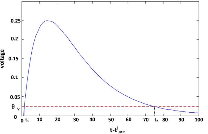
To avoid thej(sj) inEq (14)going to infinitesimal whensjis too large, not all presynaptic
spikes but only the spikes with voltagej(sj)>ϑvattdare trained, whereϑvis the voltage
threshold. Solving the same mathematical equations as Theorem 2 in the following section, the time boundaries aret1¼td tprej þt1lnðð1
ffiffiffiffiffiffiffiffiffiffiffiffiffiffiffi 1 4W
v
p
Þ=2Þand
t2¼td tjpreþt1lnðð1þ
ffiffiffiffiffiffiffiffiffiffiffiffiffiffiffi 1 4W
v
p
Þ=2Þ, as shown inFig 2. Its corresponding spike index range is denoted by [m1,m2].
If there is no input spike in the range [t1,t2],Sspikes in [t1,t2] are added randomly to the presynaptic hidden neurons with a probability. The probabilitypiassigned spikes to neuroniis
calculated by
pi¼
1
ni Pm
k¼1 1
nk
; ð16Þ
in which,mis the number of presynaptic neurons,niis the number of spikes emitted by neuron
i, andni= 0.5 if there is no spike emitted. Consequently, the fewer spikes emitted by neuroni,
the higher probabilitypiit possesses. This allocation approach not only solves the none input
problem in the training, but also balances the spike distribution. These added spikes are regarded as the target time of previous hidden layers and trained in the previous layer.
Fig 2. The voltage in the time scopet tj
pre2 ½t1;t2.The voltagej(sj) caused by the input spiketprej is aboveWvwhent tjpre2 ½t1;t2. The voltage of the inputtj
preis set to 0 at timetif thist t j
preis not in the interval [t1,t2].
Mathematical Analysis
Theoretical Derivation
In this section, the theoretical derivations in the feedforward and back propagation of our algo-rithm are presented in Theorem 1 and Theorem 2 respectively.
In traditional methods employing the temporal encoded SNNs, the output spikes of a neu-ron are detected serially in time, leading to an inefficient feed forward process. In our study, the output spike times are obtained by solving the voltage function instead of traversing all time points, which are derived in the following theorem.
Supposing that for a postsynaptic neurono, the refractory periodZðt ^t
outÞis set to A2expð ðt ^toutÞ=t1Þwith the constantA2>0, the external interference voltageuext= 0, andTpre¼ ft
1
pre;t
2
pre;t
3
pre;. . .tP 1
pregis the ordered presynaptic spike train of theP1presynaptic
input spikes, wheretj
predenotes thejth presynaptic spikes withwjrepresenting its response
syn-apse weight.mois the index of thefirst influencing spike to the postsynaptic neurono,ϑis the
firing threshold,τ1andτ2are model parameters defined inEq (2). With these definitions, the
relation between the pre and postsynaptic spikes is obtained by solving the quadratic function, which is proved in the following theorem:
Theorem 1In the SRM0model, for each range½tjpre;t jþ1
preÞin Tprewith1jP1−1,assuming that
a ¼ X
j
m¼m0
wmexpðt m
pre=t2Þ; ð17Þ
b ¼ X
j
m¼m0
wmexpðt m
pre=t1Þ A2expð^tout=t1Þ ð18Þ
If the following conditions hold:
ðIÞ a6¼0 and b2
4aW0;
ðIIÞ t1 ¼2t2;
the postsynaptic output spike toutin the range½tprej ;tjþ
1
preÞis solved by
tout¼ t1ln
b ffiffiffiffiffiffiffiffiffiffiffiffiffiffiffiffiffiffib2 4
aW
p
2a !
: ð19Þ
Proof: According to the SRM0model described in Eqs (1)–(3), fort2[tj pre;tjþ
1
pre), the voltage
of a postsynaptic neuronu(t) is
uðtÞ ¼ Zðt ^t
outÞ þ
Xj
m¼m0
wmmðt t m preÞ þu
ext:
ð20Þ
Since
(Z
ðt ^t
outÞ ¼ A2expð ðt ^toutÞ=t1Þ;
uext ¼0; ð
at timetout, we have
uðtoutÞ ¼
Xj
m¼m0
wmmðtout t m
preÞ A2exp
tout ^tout t1
: ð22Þ
The postsynaptic neuron willfire once its voltage reaches the thresholdϑ, then the postsynaptic
output spike timetoutfollows
X
j
m¼m0
wmmðtout t m
preÞ A2exp
tout ^tout t1
¼W: ð23Þ
According toEq (2),
X
j
m¼m0 wm exp
tout t m pre t1
exp tout t
m pre t2
A2exp
tout ^tout t1
¼W: ð24Þ
Thus, we have
X
j
m¼m0 wm exp
tout t1 exp t m pre t1
exp tout
t2 exp t m pre t2
A2exp
tout t1 exp ^t out t1
¼W:
ð25Þ
Suppose
z¼ exp tout t1
;
and refer to Eqs (17), (18), (25) and (II),
az2
bzþW¼0: ð26Þ
By (I), the solutions ofEq (26)is
z¼b
ffiffiffiffiffiffiffiffiffiffiffiffiffiffiffiffiffiffi
b2 4
aW
p
2a ; ð27Þ
and for all presynaptic time, we haveti>0,z>0, then
tout¼ t1ln
b ffiffiffiffiffiffiffiffiffiffiffiffiffiffiffiffiffiffi
b2 4aW p
2a !
: ð28Þ
The result follows.
The Theorem 1 proves the relation between the pre and postsynaptic spikes, which is applied to our algorithm to improve the feedforward computation efficiency.
In the feedback process of our algorithm, the error is back propagated by the presynaptic spike jitter instead of the traditional gradient decent rule, by which, the layer-wised training is applicable to our algorithm and improves the learning efficiency of our algorithm significantly. The relation of the presynaptic spike jitter and the voltage change is investigated in the follow-ing theorem.
Supposing thatΔujis the voltage variation of the postsynaptic neuronogenerated by thejth
presynaptic spike,tdis the current target spike time, and other variables are the same as that in
Theorem 1, then the relation between the time jitterDtj
preandΔujis obtained by solving the
Theorem 2In the SRM0model withτ1= 2τ2,if the voltage changeΔujfollows
ðIÞ wj 6¼0;
ðIIÞ wjjðtd tjpreÞ<Duj
1
4 jðtd t
j preÞ
wj; if wj >0
ðIIIÞ 14 jðtd t j preÞ
wj Duj < wjjðtd t j
preÞ; if wj <0
and assuming that
a ¼ wjexpððtprej tdÞ=t2Þ; ð29Þ
b ¼ wjexpððtprej tdÞ=t1Þ; ð30Þ
c ¼ wjexpððtjpre tdÞ=t2Þ wjexpððtprej tdÞ=t1Þ Duj; ð31Þ
the voltage variationΔujof the postsynaptic neuron can be achieved by the presynaptic spike
time jitter
Dtj
pre¼t1ln
b ffiffiffiffiffiffiffiffiffiffiffiffiffiffiffiffiffi
b2 4
ac p
2a
!
: ð32Þ
Proof: Supposing thatujis the postsynaptic voltage stimulated by the input spiketprej at the
target timetd, and the presynaptic spike jitter4tjpremakes the voltage change4uj. ByEq (1),
we have
wj exp tj
preþDt j pre td t1
exp t
j preþDt
j pre td t2
¼ujþDuj; ð33Þ
and then
Duj ¼ wj½exp tj
pre td t1
exp Dt
j pre t1 exp t j pre td
t1
þexp t
j pre td
t2
exp t
j pre td
t2
exp Dt
j pre t2
:
ð34Þ
Let
z¼ expðDtj
pre=t1Þ; ð35Þ
and by Eqs (29)–(31) and (34) can be expressed by
az2
þbzþc¼0: ð36Þ
Under the condition (I), we havewj6¼0)a6¼0, and ifwj>0, for condition (II),
Duj
1
4 jðtd t j preÞ
wj; ð37Þ
jðtd tj preÞ þ
Duj wj
Then the discriminant ofEq (36)is
D¼b2 4
ac ¼ w2
j exp
2 t
j pre td
t1
4w2
j exp tj
pre td t2
jðtd tjpreÞ þ Duj
wj " # w2 j exp 2 t j pre td
t1
w2
j exp tj
pre td t2
¼ w2
j exp tj t
d t2 w2 j exp tj
pre td t2
¼0:
ð39Þ
Analogously, whenwj<0, for condition (III),
Duj
1
4 jðtd t
j preÞ
wj; ð40Þ
jðtd tprej Þ þ Duj
wj
14; ð41Þ
D¼b2 4
ac0: ð42Þ
Then, under these conditions,Eq (36)has solutions
z¼ b
ffiffiffiffiffiffiffiffiffiffiffiffiffiffiffiffiffi
b2 4ac p
2a : ð43Þ
By the property of the logarithmic function, the spike jitterDtj
precan be obtained byEq (35)
only ifz>0. Forwj>0, we havea<0,b>0, then
z¼ b
ffiffiffiffiffiffiffiffiffiffiffiffiffiffiffiffiffi
b2 4
ac p
2a >
0: ð44Þ
Under condition (II), forwj>0,Duj > wjjðtd tprej Þ, we havejðtd tprej Þ þDuj=wj>0,
and then
4ac¼4w2
j exp tj
pre td t2
jðtd tprej Þ þ Duj
wj
" #
>0; ð45Þ
b2 4
ac<b2
; ð46Þ
z¼ bþ
ffiffiffiffiffiffiffiffiffiffiffiffiffiffiffiffiffi
b2 4
ac p
2a >0: ð47Þ
Analogously, by condition (III),wj<0,
z¼ b
ffiffiffiffiffiffiffiffiffiffiffiffiffiffiffiffiffi
b2 4
ac p
2a >0: ð48Þ
Then, under these conditions,Dtj
preis solved by Eqs (35) and (43) with
Dtj
pre¼t1ln
b ffiffiffiffiffiffiffiffiffiffiffiffiffiffiffiffiffi
b2 4
ac p
2a
!
: ð49Þ
Specially, whenΔujexceeds the boundary of Theorem 2 (II) or (III) in our algorithm, it is
set to the corresponding feasible boundary in the same direction of the condition.
Convergence Analysis
In this section, the convergence of our algorithm is investigated. To guarantee the convergence of the traditional and our algorithms employing the SRM0model, some conditions need to be met to select target time points. These conditions for traditional algorithms and our algorithm are studied in Theorem 3 (1) and Theorem 3 (2) respectively by analyzing the voltage function and the spiking firing conditions.
Theorem 3In the network under n layers employing the SRM0model described in Eqs(1)– (3)withτ1= 2τ2,we have:
(1) To guarantee the convergence of the traditional algorithms based on the precise spike time mechanism, a time point tm
d is available as target time only if there exist input spikes in ½tm
d ðn 1Þt1ln2;tdmÞ.
(2) To guarantee the convergence of our algorithm, a time points tm
d is available as target time only if there exist input spikes in½0;tm
dÞ.When the strategy of[t1,t2]described inFig 2is applied
to our algorithm, this scope is½tm
d nt1;tdm nt2.
Proof: (1) For an arbitraryjth input spiketjin, byEq (2),
preðt tinjÞ ¼ exp
t tinj t1
exp t t
j in t2
¼ exp t
j in t1 exp t t1 exp t j in t2 exp t t2 :
ð50Þ
Taking the partial derivatives,
@preðt tinjÞ
@t ¼
1 t1 exp t j in t1 exp t t1 þ1 t2 exp t j in t2 exp t t2
: ð51Þ
In the traditional precise time mechanism, it is@preðt tinjÞ
@t 0when emitting spikes, then we
have 1 t1 exp t j in t1 exp t t1 þ1 t2 exp t j in t2 exp t t2
0; ð52Þ
exp t t1 t t2 t2 t1
tjin t1
tjin t2
; ð53Þ
byτ1= 2τ2,
t2 t1
t1t2
t ln2þ t2 t1
t1t2
tinj; ð54Þ
ttjinþt1ln2: ð55Þ
Then in traditional algorithms, the input spiketinj can only inspire output spikes in the scope ðtinj;t
j
inþt1ln2for its postsynaptic neurons. Analogously, the output spikes caused byt
j inare
inðtjin;t j
inþ ðn 1Þt1ln2afternlayers. Consequently, traditional algorithms cannot get
con-vergent attm
convergence of the traditional algorithms based on the precise spike time mechanism, a time pointtm
d is available as target time only if there exist input spikes in½tmd ðn 1Þt1ln2;tmdÞ.
(2) Our algorithm employs the primate selective attention mechanism instead of the precise spike time rule, then there is no requirement of@preðt t
j
inÞ=@t0. When the local influence
shown inFig 2is not applied to our algorithm, all presynaptic spikes which have an influence on
tm
d can be trained to complete learning. Consequently, the time scope for input spikes is½0;t m dÞ.
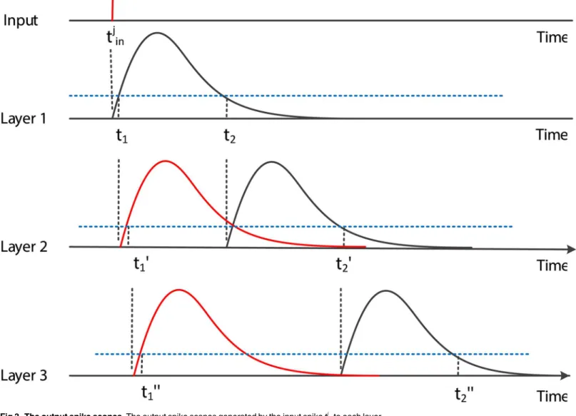
If the local influence shown inFig 2is applied to our algorithm, the time scope of output spikes generated by the inputtjinafter several layers is shown inFig 3. It is obvious that in layer
1, the time scope is [t1,t2], and in layer 2, the earliest time tofire ist10=t1+t1, and the latestfi r-ing time ist20=t2+t2. Then, for layern−1, we havetdsatisfyingEq (56)to complete training:
ðn 1Þt
1 <tdm<ðn 1Þt2 ð56Þ
Obviously, if there is no input in½tm d nt1;t
m
d nt2, thist
m
d can not be trained convergently.
Then, in this condition, the time pointstm
d is available as target time only if there exist input
spikes in½tm d nt1;t
m d nt2.
The results follow.
Theorem 3 provides conditions for encoding target times, which guarantees the conver-gence of different algorithms. It also indicates that the convergent condition of our algorithm is relaxed compared with traditional algorithms. When target spikes are selected following these conditions, different algorithms have different convergence properties and speed, which depend on their training mechanisms. In our algorithm, all qualified target times can be trained successfully and efficiently.
At themth target timetm
d, the convergence of our algorithm is proved in the Theorem 4 by
analyzing the postsynaptic voltage. Since the interference from training other target spikes or patterns varies with different network status, the following theorem proves the convergence of our algorithm ignoring this interference. The convergent situations with various interference are investigated in the following simulations sections.
Theorem 4In the SRM0model described in Eqs(1)–(3)withτ1= 2τ2,the postsynaptic voltage
of our algorithm at an arbitrary target time tm
d is convergent to the thresholdϑif the condition in Theorem 3 (2) holds, ignoring the interference from training other target spikes or patterns.
Proof: There are two cases in the training: (1) the presynaptic hidden neurons emit qualified spikes.
Since our algorithm are trained layer-wisely, each layer shares the same training process and becomes convergent in the same way. Then, the convergence of our algorithm is proved in one layer with a postsynaptic neuron and several presynaptic neurons. Suppose that the voltage of the postsynaptic neuron attm
d isuðt m
dÞcalculated byEq (1), and the voltage variations generated
by the presynaptic weight modification and spike jitter areΔuwandΔutrespectively. For an
arbitrary postsynaptic neurono, and to thepth presynaptic spike, the voltage variation gener-ated by the weight modification of this spike isDup
w, which is calculated by
Dup w¼
@uðtm dÞ @wp
Dwp; ð57Þ
whereΔwpis the variation of its weightwp. Since@uðtdmÞ=@wp¼pðtdm t p inÞ,
Dup
w¼pðtdm t p
For all presynaptic inputs, the voltage variation generated by the weight modification is
Duw¼
Xm 2
p¼m1
pðtm d t
p
preÞDwp ð59Þ
in whichtp
preis thepth presynaptic spike time, andm1andm2are thefirst and last indexes of
these presynaptic spikes. By Eqs (5), (6) and (14),
Duw¼
Xm 2
p¼m1
pðt m d t
p preÞ
rgn
pðW uðt m dÞÞ pðtm
d t p preÞ ¼
Xm 2
p¼m1 rgn
pðW uðt m
dÞÞ: ð60Þ Fig 3. The output spike scopes.The output spike scopes generated by the input spiketj
into each layer.
ByEq (15),Pm2 p¼m1g
n
p ¼1, then
Duw¼rðW uðt m
dÞÞ: ð61Þ
If the conditions in Theorem 2 hold, according toEq (8), theDtp
precalculated byEq (32)is
Dtp
pre¼t1ln
b ffiffiffiffiffiffiffiffiffiffiffiffiffiffiffiffiffi
b2 4
ac p
2a
!
; ð62Þ
which makes the postsynaptic voltage variation generated by the presynaptic spike jitterDupt
becomegpnt errnt, witherr n t andg
pn
t defined in Eqs (7) and (9) respectively. Under these
condi-tions, for all presynaptic spikes, the voltage variation inspired by the presynaptic spike jitter
Δutis
Dut¼
X
m2
p¼m1 gpn
t err n
t: ð63Þ
ByEq (9),Pm2 p¼m1g
pn
t ¼1, then according to Eqs (5) and (7),
Dut¼ ð1 rÞðW uðtmdÞÞ; ð64Þ
whereris a parameter defined inEq (7). Consequently, the whole postsynaptic voltage varia-tionΔugenerated by both presynaptic spike jitter and weight modification is
Du ¼ DutþDum¼ ð1 rÞðW uðtdmÞÞ þrðW uðt m dÞÞ
¼ W uðtm dÞ;
ð65Þ
and then
uðtm
dÞ þDu¼W: ð66Þ
If the value ofDupt exceeds the boundary in Theorem 2, the corresponding feasible boundary
value is set toDupt, and the solution is obtained according toEq (32). It is obvious that the
boundary value has the same training direction withΔu, which can makeerrclose to 0. Then our algorithm will be convergent after several leaning epochs attm
d.
(2) If there is no qualified input spike in the presynaptic hidden layer, our algorithm adds spikes randomly with probability calculated byEq (16), after which all weight modifications and spike jitters are the same as case (1), and our algorithm can get convergence.
The layer-wise training is employed in our algorithm, by which each layer shares the same training process and becomes convergent in the same way. In this analysis, the interference of other target spike trains or patterns are ignored. With the influence, our algorithm requires several more epochs to offset this interference and complete training.
The results follow.
Computational Complexity
In this section, the computational time complexity of our algorithm is studied and compared with two traditional algorithms, the SpikeProp [28] and Multi-ReSuMe [32]. Before this, the detailed pseudo-codes of the feedforward and feedback processes of our method are listed.
The Feedforward Calculation of Our Algorithm
Definition:
Tpre: the set of presynaptic spikes, which contains spikes emitted by all
pre-synaptic neuronsft1
pre;t
2
pre;t
3
pre;. . .;t P
preg.Tpreis sorted and has no duplicate
numbers.
Initialization:
The weight matrixWis initialized randomly.
Feedforward calculation:
Foreach postsynaptic neuron:
Foreach presynaptic spike intervaltj
pretot jþ1
pre with 1 <j<P−1:
For all presynaptic spikes beforetj
pre, calculate parametersaandbby
Eqs (17) and (18).
Ifaandbmeet the conditions in Theorem 1:
Calculate the output spike time in this scope byEq (19)and add it to
the output spike train of the postsynaptic neuron. End If
End For End For
Supposing that there areMpresynaptic neurons,Npostsynaptic neurons,Pinput spikes of all these presynaptic neurons, and the time length isT. As described in the pseudo-code, our algorithm detects each input spike scope and calculates parametersaandbby all of theseP
input spikes in the worst case, then the time complexity of our algorithm for one layer isO
(NP2), which also reveals the number of operations in our method.
For traditional feedforward calculation method, all discrete time points inTare detected instead of the input spike scopes ofP, then the second loop in the pseudo-code above is replaced by the time scope inT(supposing that the time interval is 1ms). For each time scope, it calculates the postsynaptic voltage by thesePinput spikes and determines whether the volt-age is greater than the threshold. In this way, the time complexity of the traditional method in one layer isO(NTP). Since a neuron can only emits one spike in a time points, we havePT. Consequently, the time complexity of our method in the feedforward calculation is less than that of the traditional approach.
Feedback modification. Similar to the feedforward calculation, the feedback weight modi-fications in each layer and each output neuron of our algorithm have the same training process. Then in this part, only the training process of one layer and one output neuron is listed in the following pseudo-code.
The Feedback Modification of Our Algorithm
Definition:
Tpre: the set of presynaptic spikes, which contains spikes emitted by all
pre-synaptic neuronsft1
pre;t
2
pre;t
3
pre;. . .;t P preg.
Td: the set of target output spikes, which contains all target spikes of the
postsynaptic neuronft1
d;t
2
d;t
3
d;. . .;t D1
d g.
Initialization:
The weight matrixWis initialized randomly.
Feedback modification:
Foreach target spike time inTd:
Calculate the weighted sum of all input spikes as the postsynaptic
volt-ageu(td), and calculate the errorerrbyEq (5).
Iferr6¼0
Step2: Calculate the presynaptic spike variation in the current layer byEq (10).
Step3: Adjust all presynaptic weights in this layer byEq (14).
End If End For
Assuming that there areMpresynaptic neurons,Npostsynaptic neurons, and the number of target spikes for all postsynaptic neurons isD, which is equal toD1+D2+. . .+DN, withDi
represents the number of target spikes of theith postsynaptic neuron. The number of input spikes isP, and the time length isT. According to the pseudo-code for the feedback modifica-tion of our algorithm, the time complexity for one layer isO(DP), which also reveals the num-ber of operations in our algorithm.
In traditional algorithms, like the SpikeProp and Multi-ReSuMe, the postsynaptic states at all time points ofTinstead of target intervalsTdare detected and their corresponding weights
are modified by a given condition. Then the time complexity for most traditional algorithms like the SpikeProp and Mullti-ReSuMe in one layer isO(TP). SinceD<T, the number of oper-ations in our algorithm is less than traditional methods.
Training Performance
In this section, the training performance of our algorithm is investigated and compared with two classical algorithms, the SpikeProp [28] and Multi-ReSuMe [32].
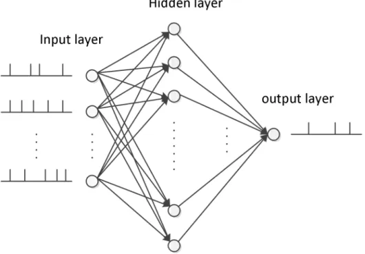
A spiking network structure employing an input layer with 50 neurons, a hidden layer with 100 spiking neurons, and an output neuron is devised in our simulations, which is shown in Fig 4. The training of the multilayer neural network consists of two steps, the feedforward
Fig 4. The network structure in our simulation.There are 50 input neurons, 100 hidden neurons, and one output neuron.
calculation and feedback weight modification. The efficiency of the both two steps is studied in the following parts.
Feedforward Calculation
The feedforward calculation is an important step before learning, it computes the output spikes from the input ones. In this subsection, two simulations are conducted to investigate the computational performance of our proposed method described in Theorem 1 compared with the traditional precise time calculation method. Specifically, the network structure is shown in Fig 4, and these input output spikes are generated by a homogeneous Poisson process.
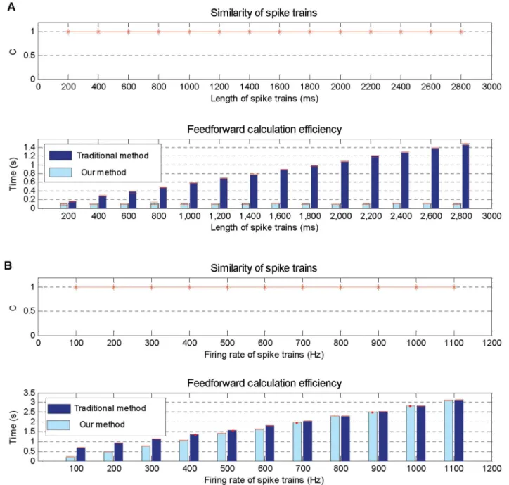
The first simulation is carried out to explore the feedforward calculation performance in dif-ferent time lengths from 200 ms to 2800 ms, and for each input neuron, one spike generated by a homogeneous Poisson process is emitted. To evaluate the similarity of the output spike trains calculated by our algorithm and traditional method quantitatively, the correlation-based mea-sureC[38] is employed, with
C¼ v1v2
jv
1jjv2j
;
wherev1v2is the inner product, and |v1|, |v2| are the Euclidean norms ofv1andv2 respec-tively. Thev1andv2are vectors obtained by the convolution of the two spike trains using a Gaussianfilter:
viðtÞ ¼
X
Ni
m¼1
exp½ ðt ti mÞ
2 =s2
;
whereNiis the number of spikes in the test spike train, andtimis themth spike in it.σis the
standard deviation of this Gaussianfilter which is set to be 1 in our study. Generally, the mea-sureCequals to 1 for identical spike trains and decrease towards zero for loosely correlated spike trains.
The simulation results are shown inFig 5A, which indicate that our proposed method has the same output spike trains as the traditional method, but achieves higher efficiency than it, because our method detects only time intervals of the input spikes instead of all time points in the traditional method.
In the second simulation, the performance of our proposed method is tested with the input firing rate of a homogeneous Poisson process ranging from 100 Hz to 1100 Hz with time length fixed to 1000 ms. Obviously, the higher the input firing rate, the higher the input densities, and when the firing rate is higher than 1000 Hz, the density of input spikes and all time points is similar.
Simulation results shown inFig 5Bindicate that our method has the same output spike trains as the traditional ones, and its computational time is growing with the increase of the input spike density. However, our method is still a little more efficient than the traditional method even if the input spike density is similar to that of all time intervals with a rate above 1000 Hz.
Feedback Weight Modification
structure depicted inFig 4. The input spike train of each input neuron is generated by a homo-geneous Poisson process withr= 10 Hz, ranging the time length from 200 ms to 2800 ms. The output neuron is desired to emit only one spike in these time lengths because the SpikeProp cannot complete training for multiple target spikes. For fast convergence of traditional algo-rithms, the target timetdis set toto+ 5, wheretois the output firing time of the first epoch.
Similar to the previous simulation,Cis employed here to measure the accuracy.
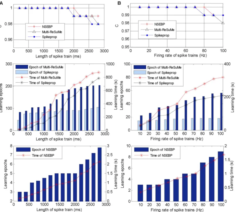
The comparison results are shown inFig 6A, in which the upper sub-figure depicts the learning accuracy of these three algorithms. It illustrates that in this simulation, our algorithm
Fig 5. Feedforward calculation performance on various situations.A: Simulation results on different time lengths ranging from 200 ms to 2800 ms. B: Simulation results on different input firing rates ranging from 10 Hz to 1100 Hz.
has a similar accuracy as traditional ones. The middle sub-figure ofFig 6Ashows the learning efficiency of the SpikeProp and the Multi-ReSuMe, and the efficiency of our algorithm is dis-played independently in the below sub-figure because the magnitude of the learning epochs and learning time of our algorithm is not the same as that of the traditional algorithms. The comparison of these two sub-figure denotes that our algorithm requires less learning epochs and learning time than the SpikeProp and Multi-ReSuMe in various situations.
Fig 6. Training performance on various situations.A: Simulation results on different time lengths fixing the input spike rate to 10 Hz. B: Simulation results on different input firing rates with the time length 500 ms.
The second simulation is conducted to test the learning efficiency of our algorithm under different firing rates, in which the input and output spike trains share the same time length of 500 ms, and the input spike train of each input neuron is generated by a homogeneous Poisson process ranging from 10 Hz to 100 Hz.
The simulation results are shown inFig 6B, where the upper sub-figure shows the accuracy of these three algorithms, the middle and the below ones depict the learning efficiency of tradi-tional algorithms and our algorithm respectively. Similar with the previous simulation, our algorithm achieves an approximate accuracy with the SpikeProp and Multi-ReSuMe, and improves the training efficiency significantly both in training epochs and training time.
To further explore the learning efficiency of these algorithms, the training time of one epoch is tested in various firing rates and time lengths. Firstly, the time length is fixed to 500 ms, and each input neuron emits a spike train generated by a homogeneous Poisson process with firing rate ranging from 10 Hz to 100 Hz, and the output neuron emits only one spike.
The simulation results shown inTable 1indicate that the higher the firing rate, the more time required for these three algorithms to complete one training epoch, since more input spikes required to be trained. Besides, our algorithm consumes less time than traditional ones in various firing rates.
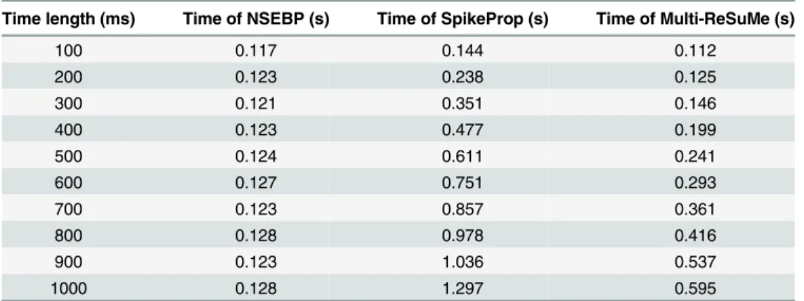
Secondly, in order to verify the effect of the time length on the training efficiency, another simulation is carried out where each input neuron emits two spikes and the output neuron emits one spike generated by a homogeneous Poisson process, and the maximum time length varies form 100 ms to 1000 ms.
The simulation results are shown inTable 2, which denotes that in various time lengths, our algorithm has the similar running time for training one epoch, while the time of the SpikeProp and Multi-ReSuMe increases obviously. This reveals the advantage of the selective attention mechanism which enables our NSEBP to concentrate attention on target contents and does not have to scan all time points as traditional algorithms do. It also indicates that the running time of NSEBP has no direct relation to the time length. These simulations in this section demon-strate that our algorithm achieves a significant improvement in efficiency compared with tradi-tional algorithms.
Non-linear Spike Pattern Classification
The XOR Benchmark
In this section, we perform experiments with the NSEBP on a classical example of a non-linear problem, the XOR benchmark to investigate its classification capability and the influence of
Table 1. Training time of one epoch for various firing rates.
Firing rate (Hz) Time of NSEBP (s) Time of SpikeProp (s) Time of Multi-ReSuMe (s)
10 0.312 0.812 0.471
20 0.441 1.255 0.814
30 0.552 1.744 1.218
40 0.634 2.185 1.598
50 0.715 2.762 2.077
60 0.746 3.278 2.468
70 0.767 3.817 2.936
80 0.771 4.496 3.422
90 0.781 5.023 3.893
100 0.794 5.591 4.314
different parameters. The network architecture shown inFig 4is employed in this section, with 4 input neurons, 10 hidden neurons and one output neuron.
The encoded method and the generation of the input spike trains are shown inFig 7. It depicts that the input 0 and 1 are encoded randomly, which is set to the spike time [1,2] and [3,4] respectively in this simulation. Then the four input patterns {0, 0}, {0, 1}, {1, 0}, {1, 1} are encoded by two segmentsS1andS2copying the encoded results of 0 and 1. The classification objects are the input spike patterns, among which the input spike trains corresponding to {0, 0} and {1, 1} are one classC1, and the input spike trains corresponding to {0, 1}, {1, 0} are the other classC2. The desired outputs of the output neuron corresponding toC1andC2are set to 10 ms and 15 ms respectively satisfying the convergent condition in Theorem 3.
Our algorithm is applied to the feed-forward network described above withϑ= 1,τ1= 5 and
r= 0.5. Different from traditional multi-layer networks in [28,32], our algorithm requires
Table 2. Training time of one epoch for various time lengths.
Time length (ms) Time of NSEBP (s) Time of SpikeProp (s) Time of Multi-ReSuMe (s)
100 0.117 0.144 0.112
200 0.123 0.238 0.125
300 0.121 0.351 0.146
400 0.123 0.477 0.199
500 0.124 0.611 0.241
600 0.127 0.751 0.293
700 0.123 0.857 0.361
800 0.128 0.978 0.416
900 0.123 1.036 0.537
1000 0.128 1.297 0.595
doi:10.1371/journal.pone.0150329.t002
Fig 7. Generation of the input spike trains.Generation of the input spike trains for the classification task in the XOR problem.
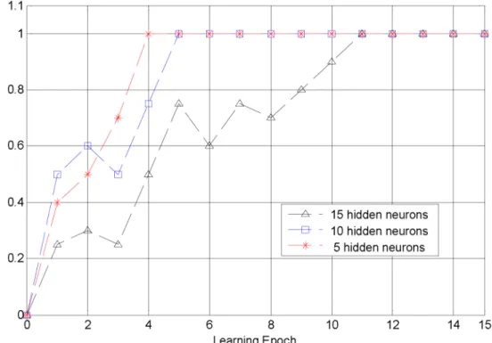
none sub-connections, which reduces the number of weight modification. With these parame-ters, our algorithm can complete training efficiently in 15 learning epochs and achieve accuracy 1 in various number of hidden neurons, as shownFig 8. This training efficiency is higher than traditional algorithms that is at least 63 epochs in Multi-ReSuMe [32] and 250 cycles in Spike-Prop [28]. In the following we systematically vary the parameters of our algorithm and investi-gate their influence.
The Parameters
In this part, we explore the influence of the parameterτ1, the number of hidden neurons, the
parameterrdefined inEq (6), and the thresholdϑon the convergent epochs. 50 simulations
are carried out and the average learning epoch is obtained.
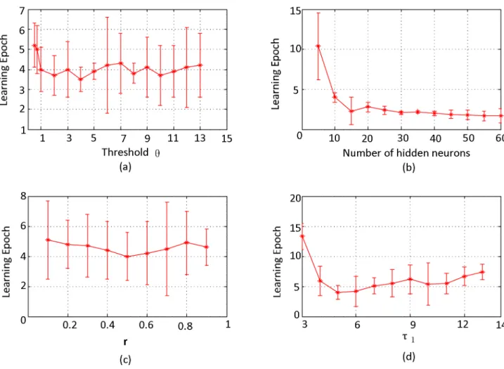
Fig 9(a)shows the convergent epochs for different values of the thresholdϑ, with the
num-ber of hidden neurons fixed to 10,r= 0.5, andτ1= 5. It suggests that the convergence of our
algorithm is insensitive to the threshold, and it can complete training in 8 epochs in various situations.
Fig 9(b)depicts the convergent epoch with different numbers of hidden neurons, which indicates that in the beginning, more neurons in the hidden layer lead to less learning epochs, while when it above 30, this change is not obvious. This is mainly because more hidden neu-rons make more sparse representation of the input patterns in the hidden layer, which are eas-ier to be trained because there is less interference between different patterns. Different amount of information requires different numbers of hidden neurons for a sparse representation, and if
Fig 8. The convergent process of our algorithm.The convergent process of our algorithm with the number of hidden neurons 5, 10, 15. All of these simulations achieve accuracy 1.
the number of hidden neurons is large enough, the variation of the convergent epoch is not apparent.
Fig 9(c)displays the convergent epoch with differentrdefined inEq (6), which determines the proportion of the error back-propagated to the previous layers. The simulation results dem-onstrate that the convergence of our algorithm has no noticeable relationship withr. To bal-ance the load of each layer, we suggestr= 1/nwhen there arenlayers required to be trained in our algorithm. In real world applications,rcan be set to different values according to different requirements.Fig 9(d)shows the convergent epoch for differentτ1, which indicates that our
algorithm can achieve rapid convergence in various cases, and different values ofτ1have some
influence on the convergent speed, but not obvious.
Simulations in this section demonstrate that our algorithm can complete non-linear classifi-cation efficiently. Besides, simulation results shown inFig 9indicate that our algorithm is not sensitive to various parameters, which makes our algorithm more convenient to be applied to various applications.
Fig 9. Convergent epochs with various parameters.Convergent epochs with various values of parameterW(a), number of hidden neurons (b), r (c), and
Classification on the UCI Datasets
In this section, we apply NSEBP to classify both the Iris and Breast Cancer Wisconsin (BCW) datasets of the UCI [39] to investigate the capability of our algorithm over classification tasks.
Iris Dataset
The Iris dataset is firstly applied to benchmark our algorithm. It contains three classes, each with 50 samples and refers to a type of the iris plant: Iris Setosa (class 1), Iris Versicolour (class 2), and Iris Virginica (class 3) [40]. Each sample contains four attributes: sepal length (feature 1), sepal width (feature 2), petal length (feature 3), and petal width (feature 4).
To make the difference between the data apparent, the data of each feature are mapped into a high dimensional space using the population time encoding method [41]. There are 12 uni-forming distributed Gaussian receptive fields in [0, 1], which distribute an input variable over 12 input neurons which are shown inFig 10.
Fig 10. Continuous input variable encoded by means of local receptive fields.The input variable is normalized to [0, 1], and a non-firing zone is defined to avoid spikes in later time. Every no firing neuron has code−1. For instance, 0.35 is encoded to a spike train of 12 neurons: (−1,−1, 14, 200,−1, 119, 7,−1, −1,−1,−1,−1).
The network structure devised for this classification task is shown inFig 11, in the iris data set, the input layer has 48 neurons with each feature 12 inputs. The hidden layer has 4 neurons, each possesses local connections with 12 neurons of the input layer that represent one feature. In the training period, only synaptic weights from input to hidden neurons are adjusted, and the output neuron has weight 1 which is applied to decision making.
In this application, theith sample of classchas the input spike traintiicfor four features and
a target spike traintdicwhich is obtained bytdic¼tiicþ2t
2ln2, with parameterτ2defined in Eq (2). The local connections in our network enable each feature to train an independent sub-network with 12 synapses. Since samples of one class have similar spike trains, encoding results reveal that there are only few different target time trains for each feature. As in the previous simulations, our algorithm chooses the class with minor voltage error.
Table 3compares the classification accuracy and convergent epoch of the NSEBP with four classical neural network classifier: Multi-ReSuMe [32], Spikeprop [28], MatlabBP, SWAT [22] for the Iris dataset on the training set and testing set. The classifier of the Multi-ReSuMe and Spikeprop are conducted with three layer SNN structures proposed in [32] and [28] respec-tively. The SWAT employs a SNN architecture of 13 input neurons with each connects to 16 neurons in middle layer, and the squared cosine encoding method is employed [22]. The simu-lation results are shown inTable 3.
The comparison results indicate that our algorithm achieves comparable or even higher accuracy compared with the traditional classifiers, while our algorithm only requires 18 epochs
Fig 11. Network structure for classification.Network structure consisting of 12Finput neurons,Fhidden neurons and one output neuron, whereFis the number of features.
to complete training, instead of 2.6106epochs for the MatlabBP, 1000 epochs for Spikeprop, 500 epochs for the SWAT, and 174 for multi-RuSuMe. The simulation results prove that our algorithm is the most efficient one, and outperforms the compared neural networks methods significantly.
Breast Cancer Wisconsin Dataset
The two-class Breast Cancer Wisconsin (BCW) dataset is also applied to analyze our algorithm. This dataset contains 699 samples, while 16 samples are abandoned because of missing data. Each sample has nine features obtained from a digitized image of a fine needle aspirate (FNA) of a breast mass [42].
The same network structure and training settings as these in the Iris classification simula-tions are employed here. There are nine features instead of four, then there are 108 input neu-rons and 9 hidden neuneu-rons in the network structure depicted inFig 11.
Table 4compares the accuracy and efficiency of the NSEBP against the existing algorithms for the BCW dataset. It shows that the test data accuracy of the NSEBP is comparable to that of the other approaches, while the NSEBP only requires 16 epochs for complete training, instead of 1500 epochs for the Spikeprop, 500 epochs for SWAT, and 9.2106epochs for MatlabBP. Then, the training efficiency of our algorithm is improved significantly compared with these classical neural network algorithms.
Simulation results in this section demonstrate that our algorithm achieves a higher effi-ciency and even a higher learning accuracy than the traditional neural network methods in the classification tasks. The selective mechanism and the presynaptic spike jitter adopted in our algorithm make the efficiency of the NSEBP to be independent with the length of the spike train, and overcome the drawbacks of low efficiency in traditional back-propagation methods. With this efficiency, the training of SNNs can meet the requirement of real world applications.
Table 3. Comparison Results for Iris Dataset.
Classifier Training accuracy Testing accuracy Training epochs
Matlab BP 0.98 0.95 2.6106
SpikeProp [28] 0.97 0.96 1000
SWAT [22] 0.95 0.95 500
Multi-ReSuMe [32] 0.96 0.94 174
NSEBP 0.98 0.96 18
doi:10.1371/journal.pone.0150329.t003
Table 4. Comparison Results for BCW Dataset.
Classifier Training accuracy Testing accuracy Training epochs
MatlabBP 0.98 0.96 9.2106
SpikeProp [28] 0.98 0.97 1500
SWAT [22] 0.96 0.96 500
NSEBP 0.97 0.96 16
Conclusion
In this paper, an efficient multi-layer supervised learning algorithm, the NSEBP, is proposed for spiking neural networks. The accurate feedforward calculation and weight modification employing the normalized PSP learning window enables our algorithm to achieve a rapid con-vergence. Besides, motivated by the selective attention mechanism of the primate visual system, our algorithm only focuses on the main contents in the target spike trains and ignores neuron states at the un-target ones, which makes our algorithm to achieve a significant improvement in efficiency of training one epoch. Simulation results demonstrate that our algorithm outper-forms traditional learning algorithms in learning efficiency, and is not sensitive to parameters. The classification results on the UCI data sets indicate that the generalization ability of our algorithm is a little better than the traditional backpropagation method, and similar to the Spi-keProp, but lower than the SWAT. It means that our algorithm does not make great contribu-tion to the over fitting problem. However, the tradicontribu-tional methods to improve the training generalization ability can also be applied to our algorithm, such as employing an optimized network structure and better decision-making method, or better sample validate methods, that will be studied in the future work.
Our algorithm is derived from the SRM0model, but the same derivation process is feasible to other models when the voltageucan be expressed by an equation of timetand can be trans-formed to a quadratic function by the substitute method. Besides, the proposed feed forward calculation method can be applied to the existing algorithms to improve their learning perfor-mance. Consequently, employing these training strategies, the SNNs can be applied efficiently to various applications with multilayer network structure and arbitrary real-valued analog inputs.
Supporting Information
S1 Table. Experiment Data for Feedforward Calculation Performance.
(XLSX)
S2 Table. Experiment Data for Training Performance with Different Time Lengths.
(XLSX)
S3 Table. Experiment Data for Training Performance with Different Firing Rates.
(XLSX)
S4 Table. Experiment Data for Training time of one epoch.
(XLSX)
S5 Table. Experiment Data for The Convergent Process of Our Algorithm with Different Number of Hidden Neurons.
(XLSX)
S6 Table. Experiment Data for The Convergent Epochs with Different Parameters.
(XLSX)
S7 Table. Experiment Data for Iris Dataset.
(XLSX)
S8 Table. Experiment Data for Breast Cancer Winsconsin Dataset.
(XLSX)
S1 File. Data Descriptions.
Acknowledgments
This work was partially supported by the National Science Foundation of China under Grants 61273308 and 61573081, and the China Scholarship Council.
Author Contributions
Conceived and designed the experiments: XX HQ. Performed the experiments: XX MZ. Ana-lyzed the data: XX GL. Contributed reagents/materials/analysis tools: XX MZ. Wrote the paper: XX JK.
References
1. Theunissen F, Miller JP. Temporal encoding in nervous systems: a rigorous definition. Journal of computational neuroscience. 1995; 2: 149–162. doi:10.1007/BF00961885PMID:8521284 2. Rullen R V, Guyonneau R, Thorpe SJ. Spike times make sense. Trends in Neurosciences. 2005; 28:
1–4. doi:10.1016/j.tins.2004.10.010
3. Hu J, Tang H, Tan KC, Li H, Shi L. A Spike-Timing-Based Integrated Model for Pattern Recognition. Neural Computation. 2013; 25: 450–472. doi:10.1162/NECO_a_00395PMID:23148414
4. O’Brien MJ, Srinivasa NA. Spiking Neural Model for Stable Reinforcement of Synapses Based on Multi-ple Distal Rewards. Neural Computation. 2013; 25:123–156. doi:10.1162/NECO_a_00387PMID: 23020112
5. Naveros F, Luque NR, Garrido JA. A Spiking Neural Simulator Integrating Event-Driven and Time-Driven Computation Schemes Using Parallel CPU-GPU Co-Processing: A Case Study. IEEE Transac-tions on Neural Networks and Learning Systems. 2015; 26: 1567–1574. doi:10.1109/TNNLS.2014. 2345844PMID:25167556
6. Zhang Z, Wu QX. Wavelet transform and texture recognition based on spiking neural network for visual images. Neurocomputing. 2015; 151: 985–995. doi:10.1016/j.neucom.2014.03.086
7. McCulloch WS, Pitts W. A logical calculus of the ideas immanent in nervous activity. The bulletin of mathematical biophysics. 1943; 5: 115–133. doi:10.1007/BF02478259
8. Rosenblatt F. The perceptron: a probabilistic model for information storage and organization in the brain. Psychological review. 1958; 65: 386. doi:10.1037/h0042519PMID:13602029
9. Tiesinga P, Fellous JM, Sejnowski TJ. Regulation of spike timing in visual cortical circuits. Nature reviews neuroscience. 2008; 9: 97–107. doi:10.1038/nrn2315PMID:18200026
10. Mehta MR, Lee AK. Role of experience and oscillations in transforming a rate code into a temporal code. Nature. 2002; 417: 741–746. doi:10.1038/nature00807PMID:12066185
11. Rullen RV, Thorpe SJ. Rate coding versus temporal order coding: What the retinal ganglion cells tell the visual cortex. Neural Computation. 2001; 13: 1255–1283. doi:10.1162/08997660152002852 PMID:11387046
12. Bohte S.M. The Evidence for Neural Information Processing with Precise Spike-times: A Survey. Natu-ral Computation. 2004; 3: 195–206. doi:10.1023/B:NACO.0000027755.02868.60
13. Benchenanel K, Peyrachel A, Khamassi M, Tierney PL, Gioanni Y, Battaglia FP, et al. Coherent theta oscillations and reorganization of spike timing in the hippocampal-prefrontal network upon learning. Neuron. 2010; 66: 921–936. doi:10.1016/j.neuron.2010.05.013
14. Gütig R, Sompolinsky H. The tempotron: a neuron that learns spike timing-based decisions. Nature neuroscience. 2006; 9: 420–428. doi:10.1038/nn1643PMID:16474393
15. Florian RV. The chronotron: a neuron that learns to fire temporally precise spike patterns. Plos one. 2012; 7: e40233. doi:10.1371/journal.pone.0040233PMID:22879876
16. Mohemmed A, Schliebs S, Matsuda S, Kasabov N. Span: Spike pattern association neuron for learning spatio-temporal spike patterns. International Journal of Neural Systems. 2012; 22: 1250012 doi:10. 1142/S0129065712500128PMID:22830962
17. Victor JD, Purpura KP. Metric-space analysis of spike trains: theory, algorithms and application. Net-work: computation in neural systems. 1997; 8: 127–164 doi:10.1088/0954-898X_8_2_003 18. van Rossum MC. A novel spike distance. Neural Computation. 2001; 13: 751–763. doi:10.1162/
089976601300014321PMID:11255567
20. Ponulak F, Kasinski A. Supervised learning in spiking neural networks with ReSuMe: sequence learn-ing, classification, and spike shifting. Neural Computation. 2010; 22: 467–510. doi:10.1162/neco. 2009.11-08-901PMID:19842989
21. Xu Y, Zeng X, Zhong S. A new supervised learning algorithm for spiking neurons. Neural computation. 2013; 25: 1472–1511. doi:10.1162/NECO_a_00450PMID:23517101
22. Wade JJ, McDaid LJ, Santos J, Sayers HM. SWAT: a spiking neural network training algorithm for clas-sification problems. IEEE Transactions on Neural Networks. 2010; 21: 1817–1830. doi:10.1109/TNN. 2010.2074212PMID:20876015
23. Yu Q, Tang H, Tan KC, Li H. Precise-spike-driven synaptic plasticity: Learning hetero-association of spatiotemporal spike patterns. Plos one. 2013; 8: e78318. doi:10.1371/journal.pone.0078318PMID: 24223789
24. Ponulak F, Kasiński A. Introduction to spiking neural networks: Information processing, learning and applications. Acta neurobiologiae experimentalis. 2010; 71: 409–433.
25. Hubel DH, Wiesel TN. Receptive fields and functional architecture of monkey striate cortex. The Jour-nal of physiology. 1968; 195: 215–243. doi:10.1113/jphysiol.1968.sp008455PMID:4966457 26. Hubel DH, Wiesel TN. Receptive fields, binocular interaction and functional architecture in the cat’s
visual cortex. The Journal of physiology. 1962; 160: 106–154 doi:10.1113/jphysiol.1962.sp006837 PMID:14449617
27. Song W, Kerr CC, Lytton WW, Francis JT. Cortical plasticity induced by spike-triggered microstimula-tion in primate somatosensory cortex. Plos one. 2013; 8(3): e57453. doi:10.1371/journal.pone. 0057453PMID:23472086
28. Bohte SM, Kok JN, La Poutre H. Error-backpropagation in temporally encoded networks of spiking neu-rons. Neurocomputing. 2002; 48: 17–37. doi:10.1016/S0925-2312(01)00658-0
29. McKennoch S, Liu D, Bushnell LG. Fast Modifications of the SpikeProp Algorithm. IEEE International Joint Conference on Neural Networks, IEEE. 2006; 48: 3970–397
30. Ghosh-Dastidara S, Adeli H. A new supervised learning algorithm for multiple spiking neural networks with application in epilepsy and seizure detection. Neural Networks. 2009; 22: 1419–1431. doi:10. 1016/j.neunet.2009.04.003
31. Xu Y, Zeng X, Han L, Yang J. A supervised multi-spike learning algorithm based on gradient descent for spiking neural networks. Neural Networks. 2013; 43: 99–113. doi:10.1016/j.neunet.2013.02.003 PMID:23500504
32. Sporea I, Grüning A. Supervised Learning in Multilayer Spiking Neural Networks. Neural Computation. 2013; 25: 473–509. doi:10.1162/NECO_a_00396PMID:23148411
33. Thorpe SJ, Imbert M. Biological constraints on connectionist modelling. Connectionism in perspective. 1989; 63–92.
34. Fink C G, Zochowski M, Booth V. Neural network modulation, dynamics, and plasticity. Global Confer-ence on Signal and Information Processing (GlobalSIP), IEEE, 2013; 843–846. doi:10.1109/ GlobalSIP.2013.6737023
35. Desimone R, Ungerleider LG. Neural mechanisms of visual processing in monkeys. Handbook of neu-ropsychology. 1989; 2: 267–299
36. Ungerleider SKALG. Mechanisms of visual attention in the human cortex. Annual Review of Neurosci-ence. 2000; 23: 315–341. doi:10.1146/annurev.neuro.23.1.315PMID:10845067
37. Gerstner W, Kistler WM. Spiking Nerual Models: Single Neurons, Populations, Plasticity. 1st ed. Cam-bridge: Cambridge University Press. 2002.
38. Schreiber S, Fellous JM. A new correlation-based measure of spike timing reliability. Neurocomputing. 2003; 52:925–931. doi:10.1016/S0925-2312(02)00838-XPMID:20740049
39. Bache K, Lichman M. UCI Machine Learning Repository; 2013. Accessed:http://archive.ics.uci.edu/ml 40. Fisher RA. The use of multiple measurements in taxonomic problems. Annals of eugenics. 1936; 7:
179–188 doi:10.1111/j.1469-1809.1936.tb02137.x
41. Snippe HP. Parameter extraction from population codes: A critical assessment. Neural Computation. 1996; 8: 511–529. doi:10.1162/neco.1996.8.3.511PMID:8868565