www.atmos-chem-phys.net/16/2381/2016/ doi:10.5194/acp-16-2381-2016
© Author(s) 2016. CC Attribution 3.0 License.
Improved simulation of tropospheric ozone by a
global-multi-regional two-way coupling model system
Yingying Yan1, Jintai Lin1, Jinxuan Chen1, and Lu Hu2
1Laboratory for Climate and Ocean-Atmosphere Studies, Department of Atmospheric and
Oceanic Sciences, School of Physics, Peking University, Beijing 100871, China
2School of Engineering and Applied Sciences, Harvard University, Cambridge, MA 02138, USA
Correspondence to:Jintai Lin ([email protected])
Received: 13 August 2015 – Published in Atmos. Chem. Phys. Discuss.: 23 September 2015 Revised: 13 January 2016 – Accepted: 11 February 2016 – Published: 29 February 2016
Abstract.Small-scale nonlinear chemical and physical pro-cesses over pollution source regions affect the tropospheric ozone (O3), but these processes are not captured by current
global chemical transport models (CTMs) and chemistry– climate models that are limited by coarse horizontal reso-lutions (100–500 km, typically 200 km). These models tend to contain large (and mostly positive) tropospheric O3biases
in the Northern Hemisphere. Here we use the recently built two-way coupling system of the GEOS-Chem CTM to sim-ulate the regional and global tropospheric O3in 2009. The
system couples the global model (at 2.5◦long.×2◦lat.) and its three nested models (at 0.667◦long.×0.5◦lat.) covering Asia, North America and Europe, respectively. Specifically, the nested models take lateral boundary conditions (LBCs) from the global model, better capture small-scale processes and feed back to modify the global model simulation within the nested domains, with a subsequent effect on their LBCs. Compared to the global model alone, the two-way coupled system better simulates the tropospheric O3both within and
outside the nested domains, as found by evaluation against a suite of ground (1420 sites from the World Data Cen-tre for Greenhouse Gases (WDCGG), the United States Na-tional Oceanic and Atmospheric Administration (NOAA) Earth System Research Laboratory Global Monitoring Divi-sion (GMD), the Chemical Coordination Centre of European Monitoring and Evaluation Programme (EMEP), and the United States Environmental Protection Agency Air Qual-ity System (AQS)), aircraft (the High-performance Instru-mented Airborne Platform for Environmental Research (HI-APER) Pole-to-Pole Observations (HIPPO) and Measure-ment of Ozone and Water Vapor by Airbus In- Service
Air-craft (MOZAIC)) and satellite measurements (two Ozone Monitoring Instrument (OMI) products). The two-way cou-pled simulation enhances the correlation in day-to-day varia-tion of afternoon mean surface O3with the ground
measure-ments from 0.53 to 0.68, and it reduces the mean model bias from 10.8 to 6.7 ppb. Regionally, the coupled system reduces the bias by 4.6 ppb over Europe, 3.9 ppb over North Amer-ica and 3.1 ppb over other regions. The two-way coupling brings O3vertical profiles much closer to the HIPPO (for
re-mote areas) and MOZAIC (for polluted regions) data, reduc-ing the tropospheric (0–9 km) mean bias by 3–10 ppb at most MOZAIC sites and by 5.3 ppb for HIPPO profiles. The two-way coupled simulation also reduces the global tropospheric column ozone by 3.0 DU (9.5 %, annual mean), bringing them closer to the OMI data in all seasons. Additionally, the two-way coupled simulation also reduces the global tro-pospheric mean hydroxyl radical by 5 % with improved es-timates of methyl chloroform and methane lifetimes. Sim-ulation improvements are more significant in the Northern Hemisphere, and are mainly driven by improved representa-tion of spatial inhomogeneity in chemistry/emissions.
1 Introduction
Tropospheric ozone (O3) is a critical pollutant and the
primary source of the hydroxyl radical (OH; the domi-nant atmospheric oxidant). Tropospheric ozone comes from stratosphere–troposphere exchange (STE) and photochemi-cal production, and is destroyed by chemiphotochemi-cal loss and dry deposition to the ground. Current global chemical transport models (CTMs) and chemistry–climate models simulate the spatiotemporal variations of ozone and its precursors, fa-cilitating a global-scale source attribution analysis to im-prove mitigation strategies (Lin et al., 2014; HTAP, 2010; Monks et al., 2015). However, most global models are lim-ited by coarse horizontal resolutions (100–500 km, typically 200 km), and they cannot resolve the fine-scale processes controlling the formation, transport and removal of ozone and its precursors. Many of these models tend to overes-timate the tropospheric ozone in the Northern Hemisphere (Lin et al., 2008; Stevenson et al., 2006; Fiore et al., 2009; Reidmiller et al., 2009; Young et al., 2013; Parrish et al., 2014). Previous studies have suggested various sources of model biases in emissions, chemical mechanisms, meteo-rological inputs and model resolutions (Wild and Prather, 2006; Lin et al., 2008; Weaver et al., 2009; J.-T. Lin et al., 2012; Doherty et al., 2013; Parrish et al., 2014; Fiore et al., 2014; Fu et al., 2015; Monks et al., 2015). Lack of capabil-ity in representing small-scale processes not resolved by the coarse-resolution global models may be an important factor for model biases, whereas the quantitative effect is much less clear, especially for the global effect of processes at scales below 100 km.
The coarse global models underrepresent many resolution-dependent processes. Ozone simulations greatly depend on horizontal resolutions due to their nonlinear dependence on concentrations of nitrogen oxides (NOx=NO+NO2) and
non-methane volatile organic compounds (NMVOCs) (Sill-man et al., 1990). Natural (biogenic and lightning) emis-sions are often calculated online by the models driven by resolution-specific meteorological conditions. Coarse-resolution global models cannot resolve the strong chemical and emission contrasts between urban and surrounding areas (Wild and Prather, 2006; Yan et al., 2014). In particular, the ozone chemistry is mostly NOxsaturated (or volatile organic
compound (VOC)-limited) in the urban areas but NOx
lim-ited in the surrounding rural regions, but the contrast is not resolved by the global model by assuming a fully mixed grid box with no sub-grid variability. Vertical transport is also res-olution dependent and not well resolved by global models by smoothing out the nearby upward and downward motions. Chen et al. (2009) showed that the global GEOS-Chem (at a∼200 km resolution) poorly represents the terrain-related
circulation around the Tibetan Plateau as the topographical feature is smoothed out. M. Lin et al. (2012a) showed that the simulated Asian influence to the US ozone is stronger with an increase in model resolution.
Several global high-resolution simulations have been con-ducted in part to enhance the representation of small-scale processes (M. Lin et al., 2012a, b; Emmons et al., 2010). For example, M. Lin et al. (2012a) used the Geophysical Fluid Dynamics Laboratory Atmospheric Model version 3 (GFDL AM3) model (at∼50 km resolution) to simulate the Asian
pollution influence for the US in May–June 2010; the high-resolution simulation was performed for 6 months. Emmons et al. (2010) used the MOZART-4 simulation (at∼70 km) to
simulate Mexican air quality in March 2006. A global high-resolution simulation is often prohibitive due to much en-hanced computational and data requirements. This is partic-ularly true for a relatively long simulation (1 year or more) that is necessary to quantify the effect of small-scale pro-cesses in different seasons and to allow for a high-resolution model spin-up period. Many high-resolution regional mod-els have also been developed that better simulate the small-scale processes in the targeted domains (e.g., Huang et al., 2008; Lin et al., 2010; Huang et al., 2010). Most of these re-gional models take the lateral boundary conditions (LBCs) of chemicals from a coarse-resolution global model without af-fecting the global model simulation, i.e., a typical “one-way” nesting setup. Thus, the improved representation of small-scale processes within the regional domain does not affect the global large-scale chemical background (simulated by the global model) that would otherwise have additional effects on the LBCs of regional models. Our previous study on car-bon monoxide (CO) demonstrated that accounting for these feedback processes enhances the simulated CO concentra-tions both within and outside the regional model domains, with a global average enhancement of 10 % (equivalent to a 25 % increase in global CO emissions) (Yan et al., 2014).
This study aims to address how the small-scale processes over the pollution source regions (not resolved by a typi-cal global model at a ∼200 km resolution) affect the
tro-pospheric O3 in the global domain, both inside and
out-side the source regions. For this purpose, we contrast the global tropospheric O3 in 2009 simulated by a
coarse-resolution global GEOS-Chem model (at 2.5◦long.×2◦lat.)
against the simulation by a recently built GEOS-Chem-based global-multi-regional two-way coupling system (Yan et al., 2014). The system uses the PeKing University Cou-PLer (PKUCPL) to integrate the global GEOS-Chem model (at 2.5◦ long.×2◦ lat.) and its three nested models (at
Figure 1. Dark green squares bounding the domains of three nested models covering Asia (70–150◦E, 11–55◦N), North Amer-ica (140–40◦W, 10–70◦N) and Europe (30◦W–50◦E, 30–70◦E). Also shown are sites of ground-level ozone measurements from WDCGG (black circle), GMD (red triangle), AQS (blue triangle) and EMEP (purple diamond); airports in the MOZAIC program for the tropospheric ozone profiles (pink square); and aircraft flight tracks in the HIPPO campaigns (red line for HIPPO-1, and green line for HIPPO-2). The overlaid map is the surface elevation (m) from a 2 min Gridded Global Relief Data (ETOPO2v2) available at NGDC Marine Trackline Geophysical database (http://www.ngdc. noaa.gov/mgg/global/etopo2.html).
between the global and nested regional models. Note that our nested model resolution is still relatively coarse com-pared to some other regional model studies (e.g., Huang et al., 2008; Lin et al., 2009; Kuhlmann et al., 2015; Ter-renoire et al., 2015); our future studies will take advan-tage of the new generation GEOS-Chem nested models at 0.3125◦long.×0.25◦lat. to capture smaller-scale processes
not resolved on a 0.667◦long.×0.5◦lat. grid.
Simulations by the coupled system and the global model alone are evaluated against a suite of ozone measurements within and outside the nested model domains from the World Data Centre for Greenhouse Gases (WDCGG), the United States National Oceanic and Atmospheric Adminis-tration (NOAA) Earth System Research Laboratory Global Monitoring Division (GMD), the Chemical Coordination Centre of European Monitoring and Evaluation Programme (EMEP), the United States Environmental Protection Agency Air Quality System (AQS), the airborne measurements from High-performance Instrumented Airborne Platform for En-vironmental Research (HIAPER) Pole-to-Pole Observations (HIPPO) campaigns, the Measurement of Ozone and Wa-ter Vapor by Airbus In- Service Aircraft (MOZAIC) aircraft program and two satellite products retrieved from the Ozone Monitoring Instrument (OMI). Surface ozone simulations are compared between the two-way system and a traditional
one-way nesting setup. Model evaluation reveals important sim-ulation improvements via the two-way coupling.
The rest of the paper is organized as follows. Section 2 describes the two-way coupled model system. Section 3 presents the ground, aircraft and OMI measurements. Sec-tion 4 compares the tropospheric budgets of ozone and re-lated species between the coupled system and the global CTM alone. The section also delineates the individual ef-fects of various chemical and non-chemical factors affect-ing the simulated ozone differences. Section 5 compares the simulated tropospheric ozone with measurements, focusing on daily, seasonal and vertical variability of ozone to demon-strate the superiority of the coupled system over the global model alone and a traditional one-way nesting setup. Sec-tion 6 concludes the present study.
2 Two-way coupled GEOS-Chem model system The current global-multi-regional two-way coupled model system (http://wiki.seas.harvard.edu/geos-chem/index. php/Two-way_coupling_between_global_and_nested_ Chem_models) is built on version 9-02 of GEOS-Chem. In this system, both the global and three nested CTMs are driven by the GEOS-5 assimilated meteorological fields from the National Aeronautic and Space Administration (NASA) Global Modeling and Assimilation Office (GMAO). The GEOS-5 data on the native 0.667◦long.×0.5◦lat. grid
are used directly to drive the nested models. To drive the global model, the meteorological data are regridded to a reduced resolution at 2.5◦long.×2◦lat. All models have 47 vertical layers, with about 10 layers of∼0.13 km thickness below 850 hPa.
In the coupling system, all global and nested models are run with the full Ox–NOx–VOC–CO–HOx gaseous
chemistry (Mao et al., 2013), the Linoz stratospheric ozone scheme (McLinden et al., 2000), and online aerosol calculations. Based on J.-T. Lin et al. (2012), we have modified the chemical mechanism as follows. The reaction constants for OH+NO2 follow Mollner et
al. (2010) for low- and high-pressure limits, i.e.,k0=1.48×
10−30×(T /300)−3cm6molecule−2s−1, and kinf=2.58×
10−11cm3molecule−1s−1. Aerosol uptake of the hydroper-oxyl radical (HO2) accounts for its self-reaction in aqueous
particles (Thornton et al., 2008). Over the continental bound-ary layer, the uptake rate is fixed at 0.07 to account for catal-ysis by transition metal ions (TMIs) (Thornton et al., 2008). Over China, however, the HO2uptake rate is assumed to be
at least 0.2 to account for the much higher fraction of TMIs in Chinese aerosols (J.-T. Lin et al., 2012); the large uptake rate is supported by recent observations (Taketani et al., 2012). The uptake of nitrogen pentoxide (N2O5) on aerosols
boundary layer (PBL) employs a non-local scheme (Holt-slag and Boville, 1993; Lin and McElroy, 2010). Model con-vection adopts the relaxed Arakawa–Schubert scheme (Rie-necker et al., 2008).
We use the Linoz stratospheric ozone scheme (McLinden et al., 2000) that produces the stratospheric ozone with rea-sonable stratosphere–troposphere exchange (STE) of ozone on an annual basis (Zhang et al., 2014). A model with a full stratospheric chemistry (e.g., M. Lin et al., 2012b; East-ham et al., 2014) would better simulate the variability of stratospheric ozone and its STE. This variability is particu-larly important for understanding the episodic ozone events (M. Lin et al., 2012b, 2015). Nevertheless, here we aim to evaluate the effect of small-scale processes within the tro-posphere on the general annual and spatial pattern of tropo-spheric ozone. Thus, a simulation with detailed stratotropo-spheric chemistry is outside the scope of this study. Also, for the STE of ozone within the nested domains, we adjust the nested model simulations to approximate the global model results by halving the Linoz ozone production rate in the strato-sphere, as we focus on the processes that affect the spheric ozone. This adjustment does not affect the tropo-spheric radiation influx, which is constrained by monthly To-tal Ozone Mapping Spectrometer Solar Backscattered Ultra-Violet (TOMS/SBUV) ozone data (http://acdb-ext.gsfc.nasa. gov/Data_services/merged/).
The two-way coupling system employs the PKUCPL cou-pler to integrate all models. Yan et al. (2014) presented a de-tailed description and evaluation of the coupling mechanism. Briefly, the coupler takes global model results for all chem-ical concentrations to update the LBCs of nested models. The coupler simultaneously replaces global model results in the troposphere within the nested domains by nested model results, after a mass-conserved area-weighted grid conver-sion procedure. The model information is exchanged every 3 h; a higher exchange frequency at 1 h leads to similar re-sults. All model simulations proceed in parallel under the two-way coupling framework. The chemistry time step is 30 min in the global model and 20 min in the nested models; and the transport time step is half of the chemistry time step for all models. Chemical and transport processes are sim-ulated in sequence: transport+chemistry+transport,
trans-port+chemistry+transport, etc.
For our focused analysis in 2009, both the two-way coupled system and the global model alone are run from July 2008 to December 2009, allowing for a 6-month spin-up period in 2008. Initial conditions of chemicals are regridded from a simulation at 5◦long.×4◦lat. conducted from 2005. All models in the two-way coupling framework proceed in parallel with eight-core (Intel(R) Xeon(R) CPU X7550 at 2.00 GHz) OpenMP parallelization for each model; a total of 32 cores are used for the coupled system and eight for the global model alone. The wall-clock time of the coupled system is slightly higher (by < 2 %) than that of the slow-est model, the North American nslow-ested model, due to some
overhead for data exchange. On this relatively old and slow computer, it takes about 15 days for the coupled system to finish 1 simulation year.
Model emissions
Table 1 summarizes the prescribed anthropogenic and biomass burning emissions. Global anthropogenic emissions are taken from the Emission Database for Global Atmo-spheric Research (EDGAR) v4.2 inventory for CO and NOx. Anthropogenic emissions of NMVOCs use as
de-fault the REanalysis of the TROpospheric chemical composi-tion (RETRO) monthly global inventory for 2000, as imple-mented by Hu et al. (2015). These global inventories are fur-ther replaced by regional inventories over Asia, North Amer-ica and Europe. Emission data include monthly or seasonal variability.
Monthly biomass burning emissions are taken from the Global Fire Emissions Database version 3 (GFED3) (van der Werf et al., 2010). Other natural emissions (lightning NOx, soil NOx, and biogenic NMVOCs) are parameterized
and calculated on-the-fly based on model meteorology; these emissions are thus resolution dependent. Soil NOx
emis-sions follow Hudman et al. (2012). Lightning NOxemissions
follow the Price and Rind scheme with a further satellite-based adjustment and a backward “C-shape” vertical pro-file (Price and Rind, 1992; Ott et al., 2010; Murray et al., 2012). Biogenic NMVOC emissions are calculated with the MEGAN v2.1 (PECCA) model (Guenther et al., 2012) driven by monthly mean MODIS leaf area index data.
Table 2 shows slight differences in global total emissions of ozone precursors (CO, NOx, and NMVOCs) between
the global model alone and the two-way coupled system. In the coupled system, global emissions from all sources are about 878 Tg yr−1 for CO, 45.5 Tg N yr−1for NOx and
723 Tg C yr−1 for NMVOCs. These values are larger than those in the global model by about 0.9, 0.7 and 6.5 %, respec-tively. Greater emission differences are found for biogenic NMVOCs (by 6.9 %) and fertilizer soil NOx(by 25.4 %),
re-flecting strong resolution dependence.
Figure 2 shows the spatial distributions of annual NMVOCs and NOx emissions in the nested models (first
and third columns) and the global model (second and fourth columns). The nested and global models exhibit similar spa-tial patterns for NMVOCs emissions. Summed over a given nested domain, the nested models have higher emissions of NMVOCs than the global model by 16–48 %, mainly a re-sult of stronger isoprene emissions. The spatial patterns of NOx emissions differ greatly between the nested and global
models, with local emission spikes much more obvious in the nested models, although the regional totals are similar (within 5 %).
The differences in model representation of NOx and
Table 1.Anthropogenic and biomass burning emission inventories used by GEOS-Chem.
Region Data set Resolutiona Year Species References and notes
Anthropogenic (fossil+biofuel) emissions
Global EDGAR
v4.2
0.1◦×0.1◦, seasonal 2008 CO, NOx, SO2 Janssens-Maenhout et al. (2010)
Global RETRO 0.5◦×0.5◦, monthly 2000 NMVOCsb http://accent.aero.jussieu.fr/RETRO_metadata.php
Global GEIA 1◦×1◦, seasonal 1990 NH3 Bouwman et al. (1997)
Global T. Bond 1◦×1◦, monthly 2000 BC, OC Bond et al. (2007)
Global AEIC
(aircraft)
1◦×1◦, annual 2005 CO, NOx,
NMVOCsb, SO2, BC, OC
Simone et al. (2013)
Asia INTEX-B 0.5◦×0.5◦, monthly 2006 CO, NOx,
NMVOCsb, SO2, BC, OC
Zhang et al. (2009)
Asia D. Streets 1◦×1◦, monthly 2000 NH3 Streets et al. (2003)
China MEIC 0.25◦×0.25◦, monthly 2008c CO, NOx,
NMVOCsb, NH3, SO2
Lin et al. (2015), Huang et al. (2012); http://www.meicmodel.org/
US NEI05 4 km×4 km, monthly
and weekend/weekday
2005c CO, NOx, NMVOCs,
NH3, SO2
ftp://aftp.fsl.noaa.gov/divisions/taq/emissions_ data_2005
Canada CAC 1◦×1◦, annual 2005c CO, NOx, NH3, SO2 http://www.ec.gc.ca/pdb/cac/cac_home_e.cfm
Mexico BRAVO 1◦×1◦, annual 1999 CO, NOx, SO2 Kuhns et al. (2003)
Europe EMEP 0.5◦×0.5◦, monthly 2005 CO, NOx,
NMVOCsb, NH3, SO2
Auvray and Bey (2005)
Biomass burning emissions
Global GFED3 0.5◦×0.5◦, monthly 2009 CO, NMVOCs, NOx,
NH3, SO2, BC, OC
van der Werf et al. (2010)
aBefore re-gridded to model horizontal resolutions. For more information, see http://wiki.seas.harvard.edu/geos-chem/index.php/Anthropogenic_emissions. bRETRO includes PRPE, C
3H8, ALK4, ALD2, CH2O and MEK; in the CTM, MEK emissions are further allocated to MEK (25 %) and ACET (75 %). AEIC, INTEX-B and MEIC
include PRPE, C2H6, C3H8, ALK4, ALD2, CH2O, MEK and ACET. NEI05 includes PRPE, C3H8, ALK4, CH2O, MEK and ACET. EMEP includes PRPE, ALK4, ALD2and
MEK. Emissions of C2H6outside Asia are from Xiao et al. (2008). cOver China, emissions of NO
xare further scaled to 2009 based on the tropospheric NO2columns from OMI measurements (Lin, et al., 2015). Over the US and Canada, emissions
of CO, NOxand SO2are scaled to 2009 (http://wiki.seas.harvard.edu/geos-chem/index.php/Scale_factors_for_anthropogenic_emissions).
Table 2.Global emissions of CO, NOxand NMVOCs in GEOS-Chem for 2009.
Total emissionsa Global model Two-way model Percentage difference
CO emissions (Tg) 869.9 877.8 0.9 %
Fossil+biofuel 500.5 504.3 0.8 %
Biomass burning 327.6 327.3 −0.1 %
NOxemissions (TgN) 45.2 45.5 0.7 %
Fossil+biofuel 27.5 27.5 0
Lightning 6.08 6.18 1.7 %
Natural soil 5.81 5.86 0.9 %
Fertilizer soil 0.71 0.89 25.4 %
Biomass burning 4.55 4.54 −0.2 %
Aircraft 0.51 0.51 0
NMVOCs emissions (TgC)b 678.4 722.7 6.5 %
Fossil+biofuel 27.8 28.1 1.1 %
Biogenic NMVOCs 640 684 6.9 %
Biomass burning 10.6 10.6 0
aSlight differences may exist between the two model frameworks in the prescribed anthropogenic (fossil+biofuel) and
biomass burning emissions, as a result of the combination of and regridding from various inventories. The consequent impacts on model simulations are negligible.
bEmitted NMVOCs include ISOP, PRPE, C
Figure 2.Total (anthropogenic+natural) emissions of NMVOCs and NOxover Asia, North America and Europe in 2009, as represented in
the nested models (0.667◦×0.5◦) and the global model (2.5◦×2◦). Values outside the upper bound of color intervals are shown in black. Color intervals are nonlinear to better present the data range; an interval without labeling represents the mean of adjacent two intervals. Also depicted in each panel is the regional total.
biogenic NMVOC in summer) affects the surface ozone sim-ulation within the nested domains (Sect. 5.1), but with a marginal effect on the global tropospheric ozone as a whole (Sect. 4.3). The better resolved emission spatial variability, as well as associated chemical contrast by the nested mod-els, greatly affects both the surface (Sect. 5.1) and the tropo-spheric ozone (Sect. 4.3, 5.2, and 5.3).
3 Ground, aircraft and OMI measurements 3.1 Ground measurements from WDCGG, GMD,
EMEP and AQS
We employ four measurement networks to evaluate the modeled ground-level ozone mixing ratios in 2009. As shown in Fig. 1, these networks contain hourly ozone measurements from a total of 1420 urban, suburban or remote sites from WDCGG (64 sites, http://ds.data. jma.go.jp/gmd/wdcgg/cgi-bin/wdcgg/catalogue.cgi), GMD (12 sites, http://www.esrl.noaa.gov/gmd/), EMEP (130 sites, http://www.nilu.no/projects/ccc/emepdata.html) and AQS (1214 sites, http://aqsdr1.epa.gov/aqsweb/aqstmp/airdata/ download_files.html). For model evaluation, we derive the afternoon (12:00–18:00 LT, local time) mean ozone mixing
ratios from the hourly data. Modeled afternoon ozone is sam-pled from the lowest layer (centered at∼0.065 km) in grid
cells covering the ground sites, and are sampled from the hourly outputs coincident with available measurements. The afternoon mean ozone is close to the maximum 8 h average ozone in both measurements (36.1 vs. 39.3 ppb averaged over the 1420 sites) and model simulations (46.8 vs. 48.4 ppb for the global model alone; 42.6 vs. 44.5 ppb for the two-way coupled system). Models also capture the diurnal cycle of measured ozone fairly well, although with positive biases in both daytime and nighttime (not shown), consistent with our previous work (Lin and McElroy, 2010).
vertical resolution) (Thouret et al., 1998). We use measure-ments taken during both takeoff and landing of the aircrafts to represent the vertical profiles over the associated airports (Zbinden et al., 2013). Each of the 11 sites chosen here has at least 40 profiles in 2009. Measurements are available from the ground level (0.075 km) to the upper troposphere and lower stratosphere (UTLS) at 0.15 km intervals. Model re-sults are sampled at times and locations consistent with the measurements.
For model evaluation in the remote areas, we use 282 ozone vertical profiles over the Pacific Ocean from two HIPPO (HIPPO-1 and HIPPO-2) aircraft campaigns con-ducted in 2009. The HIPPO campaigns were concon-ducted in the remote troposphere over the Pacific, Arctic and near-Antarctic regions to facilitate atmospheric chemistry analy-sis (Wofsy, 2011). During HIPPO, ozone was measured by the NOAA O3photometer using direct absorption at 254 nm
(Proffitt and McLaughlin, 1983; Kort et al., 2012). We use the merged data set that has a vertical resolution of 0.1 km (data available at http://hippo.ornl.gov/data_access/). To en-sure spatiotemporal consistency with the HIPPO data, model ozone is sampled at the times and locations of the measure-ments.
3.3 Two OMI products for tropospheric column ozone We use two monthly OMI tropospheric column ozone (TCO) products that have been used to study the tropospheric ozone variability and sources (Ziemke et al., 2011; Kim et al., 2013). The first product is based on an optimal estima-tion technique by Liu et al. (2007, 2010) with modifica-tions as described in Kim et al. (2013), and is referred to as OMI/LIU hereafter. For OMI/LIU, errors for individual TCO retrievals are typically 2–5 DU (Liu et al., 2010). Validation against ozonesonde data shows that mean OMI/LIU TCO agrees with ozonesonde data to within 2 DU for both the tropics (30◦S–30◦N) and northern mid-latitudes (30–60◦N), but with season-dependent biases, varying from−0.8 DU in
summer (JJA) to 2.1 DU in winter (DJF) for 30◦S–30◦N, and varying from−0.1 DU in JJA to 3 DU in DJF for 30–
60◦N (X. Liu, personal communication, 2015). The second product is the OMI/Microwave Limb Sounder (MLS) data set that subtracts the OMI total column ozone by the MLS strato-spheric ozone (Ziemke et al., 2011). Ziemke et al. (2011) val-idated the OMI/MLS data against the Southern Hemisphere Additional OZonesondes (SHADOZ) and the World Ozone and Ultraviolet radiation Data Center (WOUDC) ozonesonde measurements. They found that, on average, the monthly mean OMI/MLS tropospheric ozone mixing ratio is smaller than the ozonesonde data by about 1 ppb (2 %), with large seasonal dependence and a root mean square error at 6–8 ppb. For the present analysis, we average these two independent TCO data sets to reduce data uncertainties; this leads to a third data set referred to as OMI_MEAN.
We use the monthly mean OMI products for 2009. The OMI/LIU data set is on a 2.5◦ long.×2◦ lat. grid. The OMI/MLS product provides data at 1.25◦long.×1◦lat. from 60◦S to 60◦N. We calculate the OMI_MEAN TCO after re-gridding the OMI/MLS data to match OMI/LIU. Data polar-ward of 60◦ are discarded due to higher uncertainty. Mod-eled monthly mean TCO is calculated from all daily data at the OMI overpass time (13:00–15:00 LT) applied with the monthly mean OMI/LIU averaging kernel; daily averaging kernel data are not available, and the modeled global annual average TCO with and without applying the averaging kernel differ by 0.6 %. These OMI products and model simulations differ between each other in definitions of tropopause height and days of valid data, whose effects are found to be small. To examine the effect of different tropopause heights, we re-calculated in a test analysis the OMI/LIU, OMI_MEAN and model TCO by applying the OMI/MLS tropopause. The resulting bias of the global model relative to OMI_MEAN (2.8 DU, 8.9 %) is similar to the bias without adjusting the tropopause (2.9 DU, 9.2 %). The differences in days of valid data also have a marginal effect, as confirmed by examining the TCO difference between OMI/MLS and global model simulation sampled from days with valid OMI/MLS data (note that the OMI/MLS product also provides daily data for such analysis). The calculated TCO difference (3.9 DU; 12.8 %) is close to the difference (4.0 DU; 13.1 %) without sampling model results.
4 Effects of two-way coupling on simulated
tropospheric budgets of ozone and related species This section examines the effect of two-way coupling on the simulated tropospheric ozone budget in 2009 (Sect. 4.1), with additional discussions on NOx, CO, NMVOCs, OH
and lifetimes of methane and methyl chloroform (MCF) (Sect. 4.2). In Sect. 4.3, we delineate the chemical and non-chemical factors driving the differences between the two-way system and the global model alone.
4.1 Tropospheric ozone budget
Table 3 contrasts the global tropospheric O3 budgets in
2009 simulated by the two-way coupled system against those by the global model alone. The chemical produc-tion and loss are calculated for the odd oxygen family (Ox=O3+O+NO2+2NO3+3N2O5+PANs+HNO3+
HNO4), following Wu et al. (2007). The chemical
pro-duction of Ox is mainly driven by reactions of NO with
peroxy radicals, and the chemical loss is mostly due to the O(1D)+H2O reaction and reactions of ozone with OH
and HO2. The coupled system produces slightly higher
(by∼1.0 %) chemical loss and production of Ox than the
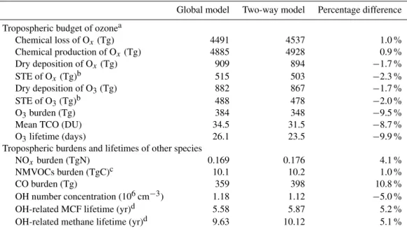
Table 3.Global tropospheric budgets of ozone and related species for 2009.
Global model Two-way model Percentage difference
Tropospheric budget of ozonea
Chemical loss of Ox(Tg) 4491 4537 1.0 %
Chemical production of Ox(Tg) 4885 4928 0.9 %
Dry deposition of Ox(Tg) 909 894 −1.7 %
STE of Ox(Tg)b 515 503 −2.3 %
Dry deposition of O3(Tg) 882 867 −1.7 %
STE of O3(Tg)b 488 478 −2.0 %
O3burden (Tg) 384 348 −9.5 %
Mean TCO (DU) 34.5 31.5 −8.7 %
O3lifetime (days) 26.1 23.5 −9.9 %
Tropospheric burdens and lifetimes of other species
NOxburden (TgN) 0.169 0.176 4.1 %
NMVOCs burden (TgC)c 10.1 10.2 1.0 %
CO burden (Tg) 359 398 10.8 %
OH number concentration (106cm−3) 1.18 1.12 −5.0 %
OH-related MCF lifetime (yr)d 5.58 5.87 5.2 %
OH-related methane lifetime (yr)d 9.63 10.12 5.1 %
aChemical production and loss rates are calculated for the odd oxygen family (O
x=O3+O+NO2+2NO3+3N2O5+PANs+
HNO3+HNO4, Wu et al., 2007), to exclude recycling reactions between O3and other Oxspecies. We note that O3accounts for over
95 % of the mass of Ox. The tropopause is defined in GEOS-5 as at the pressure where the function [0.03T−log10P] reaches its first
minimum above the surface (http://acmg.seas.harvard.edu/geos/wiki_docs/geos5/GEOS-5.2.0-File_Specification.pdf).
bStratosphere–troposphere exchange is inferred from mass balance: O
xSTE=Oxchemical loss+Oxdry deposition−Oxchemical production, and O3STE=Oxchemical loss+O3dry deposition−Oxchemical production.
cNMVOCs for burden calculation include the emitted species only: ISOP, PRPE, C
3H8, ALK4, C2H6, ALD2, CH2O, ACET and MEK. dObservation-based estimates are 10.2±0.8 (Prinn et al., 2005) or 11.2±1.3 (Prather et al., 2012) years for OH-related methane
lifetime, and 6.0±0.4 (Prinn et al., 2005) or 6.3±0.4 (Prather et al., 2012) years for OH-related MCF lifetime.
alone (882 Tg). The STE of ozone in the coupled simulation (478 Tg) is also lower than the global model alone (488 Tg) by 2.0 %, partly compensating for the weaker deposition. This small difference in STE affects the simulated global tropospheric mean ozone by 1.1 % (see Sect. 4.3).
Table 3 shows that the coupled system produces a tropo-spheric ozone burden at 348 Tg, about 9.5 % lower than the burden simulated by the global model alone (384 Tg). Cor-respondingly, the lifetime of tropospheric ozone in the cou-pled system (burden divided by sink=23.5 days) is shorter than that in the global model (26.1 days) by 9.9 %. The large reduction in ozone burden and lifetime, despite the small change in chemical production and loss of Ox, reflects a
faster chemical evolution of ozone on a per molecule basis. Although both lifetimes calculated here are broadly consis-tent with previous studies (19.9–25.5 days from ACCMIP, Young et al., 2013; and 17.3–25.9 days from ACCENT, Stevenson et al., 2006), the reduction due to our model cou-pling indicates a significant effect of small-scale processes resolved by the finer resolution, especially the fine-scale spa-tial variability of emissions and associated chemistry.
Table 4 shows the seasonal dependence of ozone burden and Ox chemical loss and production. The global model
alone produces the largest chemical loss in the Northern Hemisphere (NH) summer (1252 Tg) and the smallest loss in winter (1036 Tg). The coupled model reduces the
chem-ical loss by 1.2 % (to 1237 Tg) in NH summer, due to a lower ozone abundance overcompensating for a higher per-molecule loss rate. In winter, the coupled model en-hances the loss by 2.3 % (to 1060 Tg), because a higher per-molecule loss rate from reactions with NOxmore than offsets
a lower ozone abundance. By comparison, the coupled model slightly increases the chemical production by 0.3–1.3 % in all seasons.
4.2 NOx, CO, NMVOCs, OH, methane lifetime and
MCF lifetime
Table 3 shows that the two-way coupling also significantly affects the tropospheric burdens of ozone-related species. Burdens of NMVOCs (10.2 Tg C; see footnote of Table 3 for species included), NOx (0.176 Tg N) and CO (398 Tg)
in 2009 are higher than those simulated by the global model alone by 1.0, 4.1 and 10.8 %, respectively. Table 3 also shows that the global annual mean air-mass-weighted tropospheric OH simulated by the two-way coupled system is lower by 5.0 % than that simulated by the global model alone (1.12 vs. 1.18×106cm−3). The sensitivity of OH to model
Table 4.Global tropospheric ozone burden and Oxchemical production and loss in individual seasons of 2009.
MAM JJA SON DJF
GB TW Diff. (%) GB TW Diff. (%) GB TW Diff. (%) GB TW Diff. (%)
Chemical loss of Ox(Tg) 1087 1099 1.1 % 1252 1237 −1.2 % 1116 1141 2.2 % 1036 1060 2.3 %
Chemical production of Ox(Tg) 1197 1213 1.3 % 1446 1460 1.0 % 1199 1211 1.0 % 1042 1045 0.3 %
O3burden (Tg) 374 340 −9.1 % 394 362 −8.0 % 370 339 −8.4 % 399 352 −11.7 %
Lifetime against chemical loss (O3burden / Oxloss)
31.4 28.3 −9.8 % 28.7 26.7 −6.9 % 30.3 27.1 −10.5 % 35.1 30.3 −13.6 %
Table 3 further presents methane and MCF lifetimes due to reactions with the tropospheric OH. The lifetime calculation follows the formulae used by Yan et al. (2014); it accounts for the grid-box-specific air mass, temperature-dependent reac-tion constant, OH content and vertical gradients of methane and MCF with an adjustment coefficient of 0.97 for methane (Predoi-Cross et al., 2006) and 0.92 for MCF (Prather et al., 2012). The coupled system leads to longer lifetimes than the global model alone, by about 5.2 % (from 5.58 to 5.87 yr) for MCF and 5.1 % (from 9.63 to 10.12 yr) for methane. These results are closer to the observation-based estimates of MCF lifetime (6.0±0.4 yr from Prinn et al., 2005; 6.3±0.4 yr
from Prather et al., 2012) and methane lifetime (10.2±0.8 yr
from Prinn et al., 2005; 11.2±1.3 yr from Prather et al.,
2012).
4.3 Delineating the factors driving the difference between the two-way system and the global model alone
Compared to the global model alone, the two-way coupled system produces lower global tropospheric mean ozone by 9.5 % (Table 3). This difference is driven by four factors in-cluding the sub-coarse-grid chemical variability resolved by nested resolution (i.e., emission spatial variability and asso-ciated chemical contrast), the sub-coarse-grid variability of non-chemical factors (such as topography), a slight differ-ence in the magnitude of natural emissions (mainly for bio-genic NMVOC emissions, Sect. 2) and a slight difference in the magnitude of STE (Sect. 4.1). To delineate the individ-ual effects of these factors, we conducted three additional sensitivity simulations from July 2008 to December 2009 as follows. Results are summarized in Table 5.
The first test simulation was conducted with the global model alone, by adopting at each time step the emissions out-putted from the two-way system. Here the global model has the same emission magnitude as the two-way model, which is slightly larger than the original global model simulation (Sect. 2). As a result, the simulated global tropospheric mean ozone was enhanced by 1.1 % relative to the original global model simulation. By linear subtraction, we determine that factors other than emission magnitude lead to an ozone re-duction by 10.6 % from the global model alone to the two-way system.
The second test is the counterpart of the first test, by re-running the two-way system and adopting the emissions out-putted from the global model simulation. Here the actual resolution of emissions is 2.5◦long.×2◦lat.; thus, the sub-coarse-grid variability of emissions and associated chemical contrast is not resolved. The resulting tropospheric ozone is lower than the original global model by 2.0 %. This differ-ence represents the combined effect of the differdiffer-ence in the magnitude of STE and the sub-coarse-grid variability in non-chemical factors.
The third test addresses the slight difference in STE. The test re-run the global model but with a reduction in the STE by 1.0 %, by scaling down the Linoz stratospheric ozone pro-duction rate. As a result, the global tropospheric mean ozone is reduced by 0.55 %. By linear scaling, we determine that a 2.0 % reduction in STE from the global model to the two-way system (Table 3) would lead to a 1.1 % reduction in the global tropospheric mean ozone. Combining the result here and from the second test implies that the sub-coarse-grid non-chemical processes would reduce the global tropo-spheric mean ozone by 0.9 % from the global model alone to the two-way system.
In summary, of the −9.5 % tropospheric mean ozone
change from the global model to the two-way coupled sim-ulation, −0.9 % is related to sub-coarse-grid non-chemical
processes, −1.1 % is related to the lowered STE, +1.1 %
is associated with the increased natural emission magni-tude, and the remaining−8.6 % represents the effect of
sub-coarse-grid emission–chemical variability. Thus, the small-scale nonlinear chemical processes (resolved by the nested resolution but not by the coarse resolution) are the dominant driver of the overall ozone difference.
5 Evaluation of modeled tropospheric ozone against ground, aircraft and satellite measurements 5.1 Surface ozone
Table 5.Contributions of chemical and non-chemical factors to the change in 2009 tropospheric ozone from the global model alone to the two-way coupled system.
Factors % contribution
All factors −9.5 %
A. Higher emission magnitude (mainly related to biogenic NMVOC) +1.1 %
B. Lower STE −1.1 %
C. Nonlinear processes within the troposphere −9.5 %
C1. Small-scale chemical contrast associated with sub-coarse-grid −8.6 % variability in emissions of NOx, NMVOC, CO, etc.
C2. Non-chemical small-scale (sub-coarse-grid) processes −0.9 %
A. Obtained by contrasting simulations of the global model with vs. without adopting the nested model emissions at individual time steps; emissions are regridded from the nested to coarse resolution.
B. Obtained by perturbing the STE in the global model. C. Residual of “All factors” subtracting A and B.
C1. Residual of C subtracting C2, as driven by small-scale horizontal distributions of emissions resolved on the nested grid but not on the coarse global grid.
C2. Obtained by (1) contrasting simulations of the two-way coupled model with vs. without adopting the global model emissions at individual time steps (here emissions are regridded from the coarse to nested resolution, and are thus resolved only at the scale of the coarse grid), and then (2) subtracting B from the result of (1).
The ozone level is highest over Asia, with a value of 43.1 ppb averaged over the seven WDCGG sites. The afternoon ozone from the 17 WDCGG sites worldwide is about 33.8 ppb on average.
Figure 3 shows the horizontal distributions of annual mean afternoon ozone biases simulated by the global model alone (Fig. 3a, c and e) and by the two-way coupled system (Fig. 3b, d and f), relative to the four ground networks. All model results are derived from the global model component, i.e., from the 2.5◦long.×2◦lat. grid cell covering a given
site. The global model tends to overestimate the ozone con-centrations (biases range from −5 to 25 ppb), with a mean
bias at +10.8 ppb globally, +10.5 ppb over the US, and +12.1 ppb over Europe. The positive biases exceed 15 ppb
at several high-elevation sites of the western US (Fig. 3c) and some coastal sites of Europe (Fig. 3e). These results are broadly consistent with previous multi-model evaluation for the Hemispheric Transport of Air Pollution (HTAP) (Reid-miller et al., 2009) and Atmospheric Composition Change European Network of Excellence (ACCENT) (Dentener et al., 2006) projects that showed an ensemble mean positive bias at 10–20 ppb over the summertime eastern US and 15– 20 ppb over South Asia, respectively. Similar model biases are also found from our previous evaluation of MOZART and GEOS-Chem over the US (Lin et al., 2008; Lin and McElroy, 2010). Compared to the global model alone, the two-way coupled system generally reduces the ozone bias worldwide (Fig. 3b, d, and f). The positive bias is reduced to 6.7 ppb globally, 6.6 ppb over the US and 7.5 ppb over Europe. The bias reduction is apparent at several WDCGG sites over the North Pacific and North Atlantic (comparing Fig. 3a and b) and over the eastern US (comparing Fig. 3c and d). The two-way simulation biases against the EMEP measurements are larger than those for the EMEP/MSC-W regional CTM at a horizontal resolution of 50 km×50 km
driven by year-specific emissions (within 10 %) (http://emep. int/publ/reports/2014/sup_Status_Report_1_2014.pdf). Our higher biases are partly because the 2005 EMEP NOx
emis-sions used here are higher than those in 2009 by 25.3 % (http: //webdab.umweltbundesamt.at/official_country_trend.html). Figure 4 compares the modeled and measured day-to-day time series of regional mean afternoon ozone in 2009 for six regions in the US (from AQS) and two regions in Europe (from EMEP). The regions are defined in Fig. 3c–f, as sepa-rated by blue lines. In general, the measured ozone levels are the highest in spring and summer (Fig. 4, black lines), due to stronger STE and/or higher chemical production. Both the global model and the two-way coupled system capture the seasonal variation of measured ozone (Fig. 4, blue and red lines). The global model alone tends to overestimate the ob-servations; the annual mean bias is 9–15 ppb for any given re-gion. Seasonally, the overestimate is the largest in winter over the western US (Fig. 4a and b), in summer over the eastern US and northern Europe (Fig. 4c–g) and in fall over southern Europe (Fig. 4h). The two-way coupled simulation reduces the ozone biases in most days and regions (Fig. 4, red lines). On a seasonal mean basis, the largest reductions occur in winter (2–8 ppb for individual regions), due mainly to much enhanced titration by NOx (not shown). The bias reductions
Figure 3.Anneal mean model biases in afternoon (12:00–18:00 LT) mean ground-level ozone for the global model alone(a)and the two-way coupled model(b), with respect to measurements from WDCGG, GMD, AQS and EMEP. The symbol shapes differentiate measurement networks, consistent with Fig. 1 (circle for WDCGG, large triangle for GMD, small triangle for AQS, and diamond for EMEP). The US and European domains are enlarged in panels(c–f)to better show spatial distributions. Blue lines separate the regions presented in Fig. 4.
air aloft down to the ground (Roelofs et al., 2003; M. Lin et al., 2012b). The persistent large summertime bias may also be due to some non-resolution-dependent factors such as iso-prene nitrate chemistry and dry deposition (Lin et al., 2008; Fiore et al., 2014; Monks et al., 2015). Although the two-way coupling leads to a relatively small improvement in summer-time ground-level ozone simulations over the US and Europe (Fig. 4), the coupling results in large error reductions for tro-pospheric ozone (see Sect. 5.2 and 5.3 below).
Figure 5 compares the day-to-day time series of mod-eled afternoon ozone against the observations at 12 back-ground sites from WDCGG (panels a, b for Europe, c, d for US, e–g for Asia, h for North Pole, i for Mauna Loa in the North Pacific and j for the Southern Hemisphere). Each observation site provides a nearly complete hourly data set for model evaluation. Although the global model alone and the two-way coupled system generally overestimate the
overes-Figure 4.Day-to-day time series of afternoon (12:00–18:00 LT) mean ground-level ozone from AQS and EMEP measurements (black lines) and from model simulations (red lines for two-way coupled system, blue lines for global model alone and green lines for one-way nested models). Data are averaged over individual triangular regions indicated in Fig. 3. Numbers shown in each panel are mean model biases for annul mean, spring (MAM), summer (JJA), fall (SON) and winter (DJF).
timates in the cold seasons and much smaller biases in the warm seasons. Nevertheless, the spring–summer high values at these Asian sites are captured fairly well by both simu-lations. The spring–summer peaks are also found for other Asian regions (Lin et al., 2009; Wang et al., 2011).
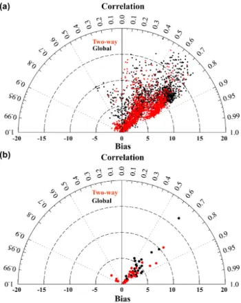
Figure 6 further presents for individual sites the day-to-day correlation and mean bias of simulated afternoon ozone relative to the observations. Figure 6a presents the results for all 1420 sites. It shows that compared to the global model alone, the two-way coupled simulation increases the correla-tion for 1179 sites and decreases the bias for 1221 sites. Av-eraged over all sites, the correlation is increased from 0.53 to 0.68, and the bias is reduced from 10.8 to 6.7 ppb. Fig-ure 6b further shows the evaluation results at the 25 sites outside the nested domains from WDCGG and GMD. The two-way coupled simulation results are within 5 ppb of the observations at 21 sites, compared to 17 sites for the global model alone. Averaged across all the 25 sites, the coupled simulation has a mean bias at 2.2 ppb and correlation at 0.74, compared to the global model bias at 4.6 ppb and correla-tion at 0.61. These results again indicate the improvement by the two-way coupling for ozone simulations both within and outside the nested domains.
Improvement of two-way coupling upon one-way nesting Within the nested domains, the two-way coupled simulation improves upon the traditional one-way nested simulations, because of the improved ozone simulation at the global scale that in turn affects the LBCs of the nested models. To il-lustrate this feedback effect, we conducted additional nested model simulations between July 2008 and December 2009 in a one-way nesting mode. Here the nested models take the LBCs from the global model without affecting the global model simulation, with other model setups the same as the nested models in the two-way coupled system. Results are regridded to 2.5◦long.×2◦lat. for consistency with the
two-way and the global model results; we note that for the com-parison in this section, the effect of this regridding is negli-gible.
The green lines in Fig. 4 show the regional average one-way nested simulation results over eight regions of the US and Europe. Compared to the global model alone (blue lines), the one-way models produce lower biases on an an-nual mean basis and for almost all seasons, reflecting the ef-fect of finer resolution prior to accounting for the improved LBCs, broadly consistent with previous regional model stud-ies (Fiore et al., 2003; Huang et al., 2008; Emery et al., 2012). The improvements are most obvious in fall and win-ter, by up to 1–2 ppb on a seasonal mean basis. The smallest differences in summer are a result of better resolved chem-ical regimes compensated by higher natural emissions and stronger vertical transport (see above discussion for two-way vs. global). The two-way coupled system (red lines) produces much smaller biases than the one-way nested simulations due
Figure 6. (a)Mean bias and day-to-day correlation of afternoon (12:00–18:00 LT) mean ground-level ozone for model simulations with respect to measurements from WDCGG, GMD, EMEP and AQS (a total of 1420 sites).(b)Similar to panel(a)but with respect to measurements outside the three nested domains from WDCGG and GMD (a total of 25 sites).
to improved LBCs. For any of these eight regions, on a re-gional annual mean basis, the amount of bias reduction (1.0– 4.0 ppb) from the one-way nesting to the two-way coupling is larger than the reduction (0.4–0.9 ppb) from the global mod-eling to the one-way nesting by a factor of 1–7. The large influence of LBCs on the one-way nested modeling was also found by previous studies (e.g., Huang et al., 2008). Our re-sults suggest that the improved LBCs through two-way cou-pling are very beneficial for the nested models.
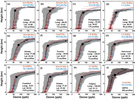
obser-Figure 7.Measured (black) and simulated (red for two-way coupled model and blue for global model alone) vertical profiles of ozone in 2009 for the MOZAIC(a–k)and HIPPO campaigns(l). MOZAIC measurements are from the ground level (0.075 km) to the UTLS at 0.15 km intervals, as averaged over all profiles. HIPPO data are averaged over all profiles at 0.1 km intervals. Model results are sampled at times and locations coincident to the measurements, except that the model vertical layers are kept for clarity. Horizontal lines indicate 1 standard deviation. Also shown in each panel are the city name, longitude, latitude, number of profiles and mean model biases below 9 km (the mean tropopause height). The black dot in each panel depicts the average tropopause height calculated from the two-way coupled model.
vations. This again indicates an important additional effect by accounting for improved LBCs via the two-way coupling.
5.2 Tropospheric ozone profile
The black lines in Fig. 7a–k show the measured vertical pro-files of tropospheric ozone averaged over 2009 at individ-ual MOZAIC sites. In general, the measured ozone increases with height, from 20–40 ppb in the lower troposphere to 40– 70 ppb at 5 km, and to larger values in the upper troposphere. For the HIPPO campaigns (black line in Fig. 7l), the average ozone mixing ratio is between 20 and 50 ppb below 9 km.
The red and blue lines in Fig. 7 show the ozone profiles simulated by the two-way coupled system and the global model alone, respectively. Here the model evaluation is fo-cused on ozone biases below 9 km, the mean tropopause height. Both simulations capture the general vertical struc-tures of MOZAIC and HIPPO ozone. Below 9 km, the global model generally overestimates the measured ozone, with a positive bias by 10.4 ppb averaged vertically and across all profiles. This overestimate is consistent with the posi-tive bias, especially north of 30◦N, reported from the AC-CENT and ACCMIP model ensemble evaluation against ozonesonde data (Stevenson at al., 2006; Young et al., 2013). The coupled system produces lower ozone concentrations in the troposphere (0–9 km) than the global model alone.
This translates to ozone bias reductions by 3–11 ppb at most MOZAIC sites (in the polluted areas) and by 5.3 ppb for HIPPO profiles (in the remote areas), averaged over 0–9 km. These improvements are a result of interactions between improved ozone simulations over pollution source regions and improved simulations of background ozone, as initially driven by a higher resolution over the source regions.
Figure 7 shows that for the MOZAIC sites, the observed ozone variability at a particular height of the profile is much larger than the modeled variability. This is because the obser-vation is sampled at every 0.15 km vertically, at a much finer resolution than the vertical resolution of the model. When the observations are mapped to the vertical resolution of the model, the observed variability is greatly reduced to a level comparable to the modeled variability (not shown).
Figure 8.Similar to Fig. 7 but for seasonal profiles at Frankfurt from the MOZAIC program.
Figure 9.Measured and modeled annual and seasonal mean tropospheric ozone columns from 60◦S to 60◦N in 2009: (from left to right) OMI/MLS, OMI retrieval by Liu et al. (2010), average of the two satellite data sets, simulation of the two-way coupled system, and simulation of the global model alone. Also shown in each panel are global, NH and SH means.
5.3 Tropospheric column ozone
Figure 9 presents the horizontal distributions of TCO in in-dividual seasons from OMI/MLS, OMI/LIU, their average OMI_MEAN, the two-way coupled system, and the global model alone. OMI/MLS and OMI/LIU produce similar sea-sonal and spatial distributions of TCO, with lower values in the tropics but higher values in the northern mid-latitudes (especially in the Northern Hemisphere (NH) summer and fall) and near 30◦S. In general, OMI/LIU produces higher TCO values than OMI/MLS by 0.8 DU (2.8 %), 1.6 DU (5.3 %), 3.8 DU (11.9 %) and 2.8 DU (9.0 %) in NH spring, summer, fall and winter, respectively. These differences are broadly consistent with the uncertainties in OMI/MLS and OMI/LIU discussed in Sect. 3.3. We thus use their average, OMI_MEAN, for model evaluation.
Figure 9 shows that both the global model alone and the coupled system reproduce the general seasonal and spatial structures of OMI_MEAN TCO. The global model tends to overestimate the seasonal TCO in OMI_MEAN, with a global mean bias of 4.4 DU (15.2 %), 3.4 DU (10.9 %), 2.2 DU (6.5 %), and 1.6 DU (4.9 %) in NH spring, summer, fall, and winter, respectively. The positive bias is more sig-nificant in the NH (annual mean bias=3.6 DU) than in the
Southern Hemisphere (SH, bias=2.2 DU). The large NH
−0.7 DU (−2.1 %) in fall and−0.7 DU (−2.2 %) in winter. The model improvements are more significant in the NH.
6 Conclusions
This study evaluates the effects on the global tropospheric ozone of nonlinear small-scale chemical and physical pro-cesses over the three major pollution source regions (Asia, North America, and Europe) not resolved by a typical global model (at a∼200 km resolution). For this purpose, we
simu-late the tropospheric ozone in 2009 simusimu-lated by a two-way coupled system integrating the global GEOS-Chem CTM (at 2.5◦long.×2◦lat.) and its three fine-resolution nested
mod-els (at 0.667◦long.×0.5◦lat.) covering Asia, North Amer-ica and Europe. The nested models better capture nonlin-ear small-scale processes within the nested domains; and the two-way coupling allows such improvements to have a global impact, which in turn improves the LBCs of the nested mod-els.
The coupled system is compared against the coarse global model alone, by employing a suite of ozone measurements in 2009 from four ground networks (WDCGG, GMD, AQS in the US, and EMEP in Europe, with 1420 sites), MOZAIC and HIPPO aircraft campaigns, and two OMI TCO products. Model evaluation clearly indicates the superiority of the two-way coupled system. Compared to the global model alone, the coupled system produces afternoon (12:00–18:00 LT) mean ground-level ozone much closer to the measurements. On an annual mean basis, the model bias is reduced by 4.1 ppb (from 10.8 to 6.7 ppb) globally, by 3.9 ppb (from 10.5 to 6.6 ppb) over the US, and by 4.6 ppb (from 12.1 to 7.5 ppb) over Europe. The coupled system also enhances the correlation to the measurements in day-to-day ozone vari-ability from 0.53 to 0.68, averaged over the 1420 sites. Al-though both the global model alone and the coupled system capture the vertical distributions of ozone measured from MOZAIC and HIPPO, the coupled system produces lower ozone values. This leads to bias reductions by 3–10 ppb at most MOZAIC sites and by 5.3 ppb for HIPPO profiles (for ozone averaged over 0–9 km). The coupled system also pro-duces lower TCO values than the global model alone, with a global annual mean reduction by 3.0 DU (9.5 %), lead-ing to better agreement with OMI data in all seasons. These model improvements are mainly driven by better representa-tion of spatially inhomogeneous nonlinear ozone chemistry associated with sub-coarse-grid spatial variability of precur-sor emissions.
Within the nested domains, the two-way coupling also leads to smaller surface ozone biases than a traditional one-way nested model setup. This is because the two-one-way cou-pling improves the ozone simulation in the global domain, which in turn improves the LBCs of the nested models. On a regional annual mean basis, the bias reduction from the one-way nesting to the two-way coupling is larger than the
reduction from the global modeling to the one-way nesting by a factor of 1–7 over the US and Europe. This result has important implications for nested/regional model studies of surface air quality.
Compared to the global model alone, the two-way cou-pled system also reduces the global tropospheric mean OH by 5.0 %, with corresponding enhancements in methane life-time (by 5.1 %), MCF lifelife-time (by 5.2 %) and CO burden (by 10.8 %). The improved quantities are closer to observation-based estimates (Prinn et al., 2005; Prather et al., 2012; Yan et al., 2014). These results are consistent with our previous analysis (Yan et al., 2014), and they point to the importance of small-scale processes to the global chemistry. Similar sulations with other global models would further test the im-portance of small-scale chemical variability for the global ozone chemistry.
At last, we note that the coupled system requires an amount of computational resource affordable for most users, i.e., 32 cores compared to eight cores for the global model alone for a similar wall-clock time. As a global high-resolution simulation is often prohibited by large computa-tional costs, we suggest a low-cost two-way coupled system integrating global and nested CTMs, like ours, to be a viable choice for most researchers.
Acknowledgements. This research is supported by the National Natural Science Foundation of China, grants 41422502 and 41175127, and the 973 program, grant 2014CB441303. We ac-knowledge the free use of ozone data from WDCGG (http://ds.data. jma.go.jp/gmd/wdcgg/), GMD (http://www.esrl.noaa.gov/gmd/),
EMEP (http://www.nilu.no/projects/ccc/emepdata.html), AQS
(http://aqsdr1.epa.gov/aqsweb/aqstmp/airdata/download_files.html),
MOZAIC-IAGOS (http://www.iagos.fr/web/), HIPPO
(http://hippo.ornl.gov/dataaccess), OMI/MLS (http://ozoneaq. gsfc.nasa.gov/) and OMI TCO data from Xiong Liu. We thank the European Commission for the support to the MOZAIC project (1994–2003) and the preparatory phase of IAGOS (2005–2012) partner institutions of the IAGOS Research Infrastructure (FZJ, DLR, MPI, KIT in Germany, CNRS, CNES, Météo-France in France and University of Manchester in United Kingdom), ETHER (CNES-CNRS/INSU) for hosting the database, the participating airlines (Lufthansa, Air France, Austrian, China Airlines, Iberia, Cathay Pacific) for the transport free of charge of the instrumenta-tion.
References
Auvray, M. and Bey, I.: Long-range transport to Europe:
seasonal variations and implications for the European
ozone budget, J. Geophys. Res.-Atmos., 110, D11303,
doi:10.1029/2004jd005503, 2005.
Bertram, T. H., Thornton, J. A., Riedel, T. P., Middlebrook, A. M., Bahreini, R., Bates, T. S., Quinn, P. K., and Coffman, D. J.: Direct observations of N2O5 reactivity on ambient aerosol particles, Geophys. Res. Lett., 36, L19803, doi:10.1029/2009gl040248, 2009.
Bond, T. C., Bhardwaj, E., Dong, R., Jogani, R., Jung, S., Ro-den, C., Streets, D. G., and Trautmann, N. M.: Historical emis-sions of black and organic carbon aerosol from energy-related combustion, 1850–2000, Global Biogeochem. Cy., 21, GB2018, doi:10.1029/2006GB002840, 2007.
Bouwman, A. F., Lee, D. S., Asman, W. A. H., Dentener, F. J., Van Der Hoek, K. W., and Olivier, J. G. J.: A global high-resolution emission inventory for ammonia, Global Biogeochem. Cy., 11, 561–587, 1997.
Chen, D., Wang, Y., McElroy, M. B., He, K., Yantosca, R. M., and Le Sager, P.: Regional CO pollution and export in China simu-lated by the high-resolution nested-grid GEOS-Chem model, At-mos. Chem. Phys., 9, 3825–3839, doi:10.5194/acp-9-3825-2009, 2009.
Dentener, F., Stevenson, D., Ellingsen, K., van Noije, T., Schultz, M., Amann, M., Atherton, C., Bell, N., Bergmann, D., Bey, I., Bouwman, L., Butler, T., Cofala, J., Collins, B., Drevet, J., Do-herty, R., Eickhout, B., Eskes, H., Fiore, A., Gauss, M., Hauglus-taine, D., Horowitz, L., Isaksen, I. S. A., Josse, B., Lawrence, M., Krol, M., Lamarque, J. F., Montanaro, V., Muller, J. F., Peuch, V. H., Pitari, G., Pyle, J., Rast, S., Rodriguez, J., Sanderson, M., Savage, N. H., Shindell, D., Strahan, S., Szopa, S., Sudo, K., Van Dingenen, R., Wild, O., and Zeng, G.: The global atmospheric environment for the next generation, Environ. Sci. Technol., 40, 3586–3594, doi:10.1021/es0523845, 2006.
Doherty, R. M., Wild, O., Shindell, D. T., Zeng, G., MacKenzie, I. A., Collins, W. J., Fiore, A. M., Stevenson, D. S., Dentener, F. J., Schultz, M. G., Hess, P., Derwent, R. G., and Keating, T. J.: Impacts of climate change on surface ozone and intercontinental ozone pollution: A multi-model study, J. Geophys. Res.-Atmos., 118, 3744–3763, doi:10.1002/jgrd.50266, 2013.
Eastham, S. D., Weisenstein, D. K., and Barrett, S. R. H.: Development and evaluation of the unified tropospheric-stratospheric chemistry extension (UCX) for the global chemistry-transport model GEOS-Chem, Atmos. Environ., 89, 52–63, doi:10.1016/j.atmosenv.2014.02.001, 2014.
Emery, C., Jung, J., Downey, N., Johnson, J., Jimenez, M., Yarvvood, G., and Morris, R.: Regional and global modeling estimates of policy relevant background ozone over the United States, Atmos. Environ., 47, 206–217, doi:10.1016/j.atmosenv.2011.11.012, 2012.
Emmons, L. K., Apel, E. C., Lamarque, J.-F., Hess, P. G., Avery, M., Blake, D., Brune, W., Campos, T., Crawford, J., DeCarlo, P. F., Hall, S., Heikes, B., Holloway, J., Jimenez, J. L., Knapp, D. J., Kok, G., Mena-Carrasco, M., Olson, J., O’Sullivan, D., Sachse, G., Walega, J., Weibring, P., Weinheimer, A., and Wiedinmyer, C.: Impact of Mexico City emissions on regional air quality from MOZART-4 simulations, Atmos. Chem. Phys., 10, 6195–6212, doi:10.5194/acp-10-6195-2010, 2010.
Evans, M. J. and Jacob, D. J.: Impact of new laboratory studies of N2O5 hydrolysis on global model budgets of tropospheric nitro-gen oxides, ozone, and OH, Geophys. Res. Lett., 32, L09813, doi:10.1029/2005gl022469, 2005.
Fiore, A. M., Jacob, D. J., Mathur, R., and Martin, R. V.: Applica-tion of empirical orthogonal funcApplica-tions to evaluate ozone simula-tions with regional and global models, J. Geophys. Res.-Atmos., 108, 4431, doi:10.1029/2002jd003151, 2003.
Fiore, A. M., Dentener, F. J., Wild, O., Cuvelier, C., Schultz, M. G., Hess, P., Textor, C., Schulz, M., Doherty, R. M., Horowitz, L. W., MacKenzie, I. A., Sanderson, M. G., Shindell, D. T., Stevenson, D. S., Szopa, S., Van Dingenen, R., Zeng, G., Ather-ton, C., Bergmann, D., Bey, I., Carmichael, G., Collins, W. J., Duncan, B. N., Faluvegi, G., Folberth, G., Gauss, M., Gong, S., Hauglustaine, D., Holloway, T., Isaksen, I. S. A., Jacob, D. J., Jonson, J. E., Kaminski, J. W., Keating, T. J., Lupu, A., Marmer, E., Montanaro, V., Park, R. J., Pitari, G., Pringle, K. J., Pyle, J. A., Schroeder, S., Vivanco, M. G., Wind, P., Wojcik, G., Wu, S., and Zuber, A.: Multimodel estimates of intercontinental source-receptor relationships for ozone pollution, J. Geophys. Res., 114, D04301, doi:10.1029/2008jd010816, 2009.
Fiore, A. M., Oberman, J. T., Lin, M. Y., Zhang, L., Clifton, O. E., Jacob, D. J., Naik, V., Horowitz, L. W., and Pinto, J. P.: Estimating North American background ozone in US sur-face air with two independent global models: Variability, uncer-tainties, and recommendations, Atmos. Environ., 96, 284–300, doi:10.1016/j.atmosenv.2014.07.045, 2014.
Fu, T.-M., Zheng, Y., Paulot, F., Mao, J., and Yantosca, R. M.: Pos-itive but variable sensitivity of August surface ozone to large-scale warming in the southeast United States, Nature Climate Change, 5, 454–458, doi:10.1038/nclimate2567, 2015.
Guenther, A. B., Jiang, X., Heald, C. L., Sakulyanontvittaya, T., Duhl, T., Emmons, L. K., and Wang, X.: The Model of Emissions of Gases and Aerosols from Nature version 2.1 (MEGAN2.1): an extended and updated framework for modeling biogenic emis-sions, Geosci. Model Dev., 5, 1471–1492, doi:10.5194/gmd-5-1471-2012, 2012.
Holtslag, A. A. M. and Boville, B. A.: Local Versus
Non-local Boundary-Layer Diffusion in a Global Climate
Model, J. Climate, 6, 1825–1842,
doi:10.1175/1520-0442(1993)006<1825:LVNBLD>2.0.CO;2, 1993.
HTAP: Hemispheric Transport of Air Pollution 2010 Executive Summary ECE/EB.AIR/2010/10 Corrected, United Nations, available at: http://www.htap.org/publications/2010_report/ 2010_Final_Report/EBMeeting2010.pdf (last access: 1 Febru-ary 2015), 2010.
Hu, L., Millet, D. B., Baasandorj, M., Griffis, T. J., Travis, K. R., Tessum, C. W., Marshall, J. D., Reinhart, W. F., Mikoviny, T., Mueller, M., Wisthaler, A., Graus, M., Warneke, C., and de Gouw, J.: Emissions of C6C8aromatic compounds in the United States: Constraints from tall tower and air-craft measurements, J. Geophys. Res.-Atmos., 120, 826–842, doi:10.1002/2014jd022627, 2015.
Huang, M., Carmichael, G. R., Adhikary, B., Spak, S. N., Kulkarni, S., Cheng, Y. F., Wei, C., Tang, Y., Parrish, D. D., Oltmans, S. J., D’Allura, A., Kaduwela, A., Cai, C., Weinheimer, A. J., Wong, M., Pierce, R. B., Al-Saadi, J. A., Streets, D. G., and Zhang, Q.: Impacts of transported background ozone on California air qual-ity during the ARCTAS-CARB period – a multi-scale modeling study, Atmos. Chem. Phys., 10, 6947–6968, doi:10.5194/acp-10-6947-2010, 2010.
Huang, X., Song, Y., Li, M., Li, J., Huo, Q., Cai, X., Zhu, T., Hu, M., and Zhang, H.: A high-resolution ammonia emis-sion inventory in China, Global Biogeochem. Cy., 26, GB1030, doi:10.1029/2011gb004161, 2012.
Hudman, R. C., Moore, N. E., Mebust, A. K., Martin, R. V., Russell, A. R., Valin, L. C., and Cohen, R. C.: Steps towards a mechanistic model of global soil nitric oxide emissions: implementation and space based-constraints, Atmos. Chem. Phys., 12, 7779–7795, doi:10.5194/acp-12-7779-2012, 2012.
Janssens-Maenhout, G., Petrescu, A. M. R., Muntean, M., and Blu-jdea, V.: Verifying Greenhouse Gas Emissions: Methods to Sup-port International Climate Agreements, The National Academies Press, 124 pp., 132–133, doi:10.1080/20430779.2011.579358, 2010.
Kim, P. S., Jacob, D. J., Liu, X., Warner, J. X., Yang, K., Chance, K., Thouret, V., and Nedelec, P.: Global ozone-CO correlations from OMI and AIRS: constraints on tropospheric ozone sources, Atmos. Chem. Phys., 13, 9321–9335, doi:10.5194/acp-13-9321-2013, 2013.
Kort, E. A., Wofsy, S. C., Daube, B. C., Diao, M., Elkins, J. W., Gao, R. S., Hintsa, E. J., Hurst, D. F., Jimenez, R., Moore, F. L., Spackman, J. R., and Zondlo, M. A.: Atmospheric observations of Arctic Ocean methane emissions up to 82 degrees north, Nat. Geosci., 5, 318–321, doi:10.1038/ngeo1452, 2012.
Kuhlmann, G., Lam, Y. F., Cheung, H. M., Hartl, A., Fung, J. C. H., Chan, P. W., and Wenig, M. O.: Development of a cus-tom OMI NO2data product for evaluating biases in a regional chemistry transport model, Atmos. Chem. Phys., 15, 5627–5644, doi:10.5194/acp-15-5627-2015, 2015.
Kuhns, H., Etyemezian, V., Green, M., Hendrickson, K., McGown, M., Barton, K., and Pitchford, M.: Vehicle-based road dust emis-sion measurement – Part II: Effect of precipitation, wintertime road sanding, and street sweepers on inferred PM10 emission potentials from paved and unpaved roads, Atmos. Environ., 37, 4573–4582, doi:10.1016/s1352-2310(03)00529-6, 2003. Lin, J.-T. and McElroy, M. B.: Impacts of boundary layer mixing
on pollutant vertical profiles in the lower troposphere: Impli-cations to satellite remote sensing, Atmos. Environ., 44, 1726– 1739, doi:10.1016/j.atmosenv.2010.02.009, 2010.
Lin, J.-T., Youn, D., Liang, X. Z., and Wuebbles, D. J.: Global model simulation of summertime US ozone diur-nal cycle and its sensitivity to PBL mixing, spatial res-olution, and emissions, Atmos. Environ., 42, 8470–8483, doi:10.1016/j.atmosenv.2008.08.012, 2008.
Lin, J.-T., Liu, Z., Zhang, Q., Liu, H., Mao, J., and Zhuang, G.: Modeling uncertainties for tropospheric nitrogen dioxide columns affecting satellite-based inverse modeling of nitro-gen oxides emissions, Atmos. Chem. Phys., 12, 12255–12275, doi:10.5194/acp-12-12255-2012, 2012.
Lin, J.-T., Pan, D., Davis, S. J., Zhang, Q., He, K., Wang, C., Streets, D. G., Wuebbles, D. J., and Guan, D.: China’s international trade
and air pollution in the United States, P. Natl. Acad. Sci. USA, 111, 1736–1741, doi:10.1073/pnas.1312860111, 2014.
Lin, M., Holloway, T., Oki, T., Streets, D. G., and Richter, A.: Multi-scale model analysis of boundary layer ozone over East Asia, At-mos. Chem. Phys., 9, 3277–3301, doi:10.5194/acp-9-3277-2009, 2009.
Lin, M., Holloway, T., Carmichael, G. R., and Fiore, A. M.: Quan-tifying pollution inflow and outflow over East Asia in spring with regional and global models, Atmos. Chem. Phys., 10, 4221– 4239, doi:10.5194/acp-10-4221-2010, 2010.
Lin, M., Fiore, A. M., Horowitz, L. W., Cooper, O. R., Naik, V., Holloway, J., Johnson, B. J., Middlebrook, A. M., Oltmans, S. J., Pollack, I. B., Ryerson, T. B., Warner, J. X., Wiedinmyer, C., Wilson, J., and Wyman, B.: Transport of Asian ozone pollution into surface air over the western United States in spring, J. Geo-phys. Res., 117, D00V07, doi:10.1029/2011JD016961, 2012a. Lin, M., Fiore, A. M., Cooper, O. R., Horowitz, L. W., Langford,
A. O., Levy II., H., Johnson, B. J., Naik, V., Oltmans, S. J., and Senff, C.: Springtime high surface ozone events over the western United States: Quantifying the role of stratospheric intrusions, J. Geophys. Res., 117, D00V22, doi:10.1029/2012JD018151, 2012b.
Lin, M., Fiore, A. M., Horowitz, L. W., Langford, A. O., Oltmans, S. J., Tarasick, D., and Rieder, H. E.: Climate variability modulates western US ozone air quality in spring via deep stratospheric in-trusions, Nat. Comm., 6, 7105, doi:10.1038/ncomms8105, 2015. Liu, X., Chance, K., and Kurosu, T. P.: Improved ozone profile retrievals from GOME data with degradation correction in re-flectance, Atmos. Chem. Phys., 7, 1575–1583, doi:10.5194/acp-7-1575-2007, 2007.
Liu, X., Bhartia, P. K., Chance, K., Spurr, R. J. D., and Kurosu, T. P.: Ozone profile retrievals from the Ozone Monitoring Instrument, Atmos. Chem. Phys., 10, 2521–2537, doi:10.5194/acp-10-2521-2010, 2010.
Mao, J., Paulot, F., Jacob, D. J., Cohen, R. C., Crounse, J. D., Wennberg, P. O., Keller, C. A., Hudman, R. C., Barkley, M. P., and Horowitz, L. W.: Ozone and organic nitrates over the east-ern United States: Sensitivity to isoprene chemistry, J. Geophys. Res.-Atmos., 118, 11256–11268, doi:10.1002/jgrd.50817, 2013. Marenco, A., Thouret, V., Nedelec, P., Smit, H., Helten, M., Kley, D., Karcher, F., Simon, P., Law, K., Pyle, J., Poschmann, G., Von Wrede, R., Hume, C., and Cook, T.: Measurement of ozone and water vapor by Airbus in-service aircraft: The MOZAIC airborne program, An overview, J. Geophys. Res.-Atmos., 103, 25631– 25642, doi:10.1029/98jd00977, 1998.
McLinden, C. A., Olsen, S. C., Hannegan, B., Wild, O., Prather, M. J., and Sundet, J.: Stratospheric ozone in 3-D models: A sim-ple chemistry and the cross-tropopause flux, J. Geophys. Res.-Atmos., 105, 14653–14665, doi:10.1029/2000jd900124, 2000. Mollner, A. K., Valluvadasan, S., Feng, L., Sprague, M. K.,