What can we learn about ship emission inventories from measurements of air pollutants over the Mediterranean Sea?

(1)

ACPD

9, 7155–7211, 2009

What can we learn about ship emission

inventories?

E. Marmer et al.

Title Page

Abstract Introduction

Conclusions References

Tables Figures

◭ ◮

Back Close

Full Screen / Esc

Printer-friendly Version

Interactive Discussion Atmos. Chem. Phys. Discuss., 9, 7155–7211, 2009

www.atmos-chem-phys-discuss.net/9/7155/2009/ © Author(s) 2009. This work is distributed under the Creative Commons Attribution 3.0 License.

Atmospheric Chemistry and Physics Discussions

This discussion paper is/has been under review for the journalAtmospheric Chemistry and Physics (ACP). Please refer to the corresponding final paper inACPif available.

What can we learn about ship emission

inventories from measurements of air

pollutants over the Mediterranean Sea?

E. Marmer1, F. Dentener1, J. v. Aardenne1, F. Cavalli1, E. Vignati1, K. Velchev1, J. Hjorth1, F. Boersma2, G. Vinken3, N. Mihalopoulos4, and F. Raes1

1

European Commission, Joint Research Centre, Institute of Environment and Sustainability, via E. Fermi, 2749, 21027 Ispra, Italy

2

KNMI, Climate Observations Department, Wilhelminalaan 10, 3732 GK De Bilt, The Netherlands

3

Eindhoven University of Techology, Bezoekadres, Den Dolech 2 5612 AZ Eindhoven, The Netherlands

4

University of Crete, Department of Chemistry, 71003 Heraklion, Greece

Received: 6 February 2009 – Accepted: 2 March 2009 – Published: 17 March 2009 Correspondence to: E. Marmer (elina.marmer@jrc.it)

(2)

ACPD

9, 7155–7211, 2009

inventories?

E. Marmer et al.

Title Page

Tables Figures

◭ ◮

Back Close

Full Screen / Esc

Interactive Discussion

Abstract

Ship emission estimates diverge widely for all chemical compounds for several rea-sons: use of different methodologies (bottom-up or top-down), activity data and emis-sion factors can easily result in a difference from a factor of 1.5 to two orders of mag-nitude. Despite these large discrepancies in existing ship emission inventories for air 5

pollutants very little has been done to evaluate their consistency with atmospheric mea-surements at open sea. Combining three sets of observational data – ozone and black carbon measurements sampled at three coastal sites and on board of a Mediterranean cruise ship, as well as satellite observations of atmospheric NO2column concentration

over the same area – we assess the accuracy of the three most commonly used ship 10

emission inventories, EDGAR FT (Olivier et al., 2005), emissions described by Eyring et al. (2005) and emissions reported by EMEP (Vestreng et al., 2007). Our tool is a global atmospheric chemistry transport model which simulates the chemical state of the Mediterranean atmosphere applying di_fferent ship emission inventories. The simu-lated contributions of ships to air pollutant levels in the Mediterranean atmosphere are 15

significant but strongly depend on the inventory applied. Close to the major shipping routes relative contributions vary from 10 to 50% for black carbon and from 2 to 12% for ozone in the surface layer, as well as from 5 to 20% for nitrogen dioxide atmospheric column burden. The relative contributions are still significant over the North African coast, but less so over the South European coast. The observations poorly constrain 20

the ship emission inventories in the Eastern Mediterranean where the influence of un-certain land based emissions, the model transport and wet deposition are at least as important as the signal from ships. In the Western Mediterranean, the regional EMEP emission inventory gives the best match with most measurements, followed by Eyring for NO2 and ozone and by EDGAR for black carbon. Given the uncertainty of the

25

(3)

ACPD

9, 7155–7211, 2009

inventories?

E. Marmer et al.

Title Page

Tables Figures

◭ ◮

Back Close

Full Screen / Esc

1 Introduction

Ship emissions and their impacts on environment became a “hot” issue in the past decade for atmospheric research and air pollution and climate policy. Recent publica-tions on health impacts of particles emitted by ships (Corbett et al., 2007a), acidifica-tion and eutroficaacidifica-tion of water and soil in coastal regions caused by sulfur and nitrogen 5

deposition (Derwent at al., 2005), climate cooling owing to the high sulfur content of marine fuel (Devasthale et al., 2006; Laurer et al., 2007), climate warming caused by the emissions of GHGs (Stern, 2007) and absorbing black carbon (Lack et al., 2008), to name just a few, contributed to our knowledge of present environmental impacts of this steadily growing emission source. They also raised public awareness and put a grow-10

ing pressure on policy makers to find an international agreement on ship emission reg-ulations, as ship emissions are known to be one of the least regulated anthropogenic sources (Eyring et al., 2005). In Europe, where the land based emissions of sulfur have been successfully reduced since 1980’s, the ships are the only growing source of sulfur emissions. Unless more action is taken, by the year 2020 sulfur and nitrogen 15

emissions from ships threaten to exceed all European land sources combined (CAFE, 2005), with a similar situation in the USA (ARB, 2006). International shipping is a major source of sulfur emissions in Asia because the rapid growth of Asian economies results in a corresponding growth of shipping trade (Streets et al., 1997, 2003). Last year, the International Maritime Organization (IMO) unanimously adopted amendments to the 20

MARPOL Annex VI regulations to reduce SOx, NOx and particulate emissions from

ships (IMO, 2008). The revised Annex VI will enter into force in July 2010. In support of the policy, research is required to investigate how the implementation of these regu-lations, combined with the predicted future growth of ship traffic and the geographical expansion of waterways and ports are going to affect the atmospheric composition. 25

(4)

emis-ACPD

9, 7155–7211, 2009

inventories?

E. Marmer et al.

Title Page

Tables Figures

◭ ◮

Back Close

Full Screen / Esc

Interactive Discussion sion estimates in total and for different compounds. These differences are caused by

di_fferent methodologies as well as uncertainties in the emission factors. For instance, European inventories tend to give a higher estimate for the European regions than the global inventories (Wang et al., 2008), mainly because domestic shipping is not rep-resented in the activity data on which the global inventories are based. Verification of 5

the consistency of ship emissions inventories with observations is a difficult task due to lack of observations over the open sea.

We evaluate three widely used ship emission inventories – EDGAR FT 2000 (Olivier et al., 2005), Eyring et al. (2005) and EMEP (Vestreng et al., 2007) – by implementing them in a chemistry transport model TM5 (Krol et al., 2005) and comparing the results 10

with available observations. Our focus is on the Mediterranean Sea, first of all because its atmosphere appears to be one of the most polluted in the world (Kouvarakis et al., 2000; Lelieveld and Dentener, 2000) and significant contribution of the very dense ship tra_ffic connecting the Atlantic and the Indian Oceans is to be expected. Inland seas with intense transit and local ship traffic and high population density are especially 15

affected by ship emissions, as found i.e. over the Mediterranean (Marmer and Lang-mann, 2005) and the Marmara Sea (Deniz and Durmuso ˆglu, 2008). The second not less important reason is the fact that here we have a unique set of observational data from continuous onboard ship measurements (Velchev et al., 2009). In addition, the observations obtained from the OMI satellite over this area are for the first time used 20

to constrain ship emissions.

Finally we present a new global ship emission inventory EDGARv4 aimed to consol-idate the advantages and disadvantages of the regional and global inventories.

2 Ship emission inventories

We have examined six different ship emission inventories focusing on the Mediter-25

(5)

ACPD

9, 7155–7211, 2009

inventories?

E. Marmer et al.

Title Page

Tables Figures

◭ ◮

Back Close

Full Screen / Esc

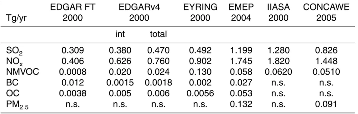
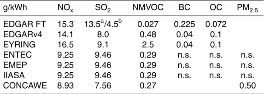
Interactive Discussion (CO) and non methane volatile organic carbons (NMVOCs). While in global inventories

carbonaceous particles such as black and organic carbon (BC and OC) are included explicitly, the regional inventories give the particulate emissions as PM2.5 (Table 1).

For this study we have applied the speciation based on Anersson-Skøld and Simpson (2001), attributing 40% of the total PM2.5 to OC and 20% to BC (the remaining 40%

5

assumed to be inorganics).

The global emission inventories EDGAR FT 2000 (Olivier et al., 2005, with OC and BC emissions based on Bond et al., 2004), later referred to as EDGAR, and Eyring et al. (2005), later referred to as Eyring, both compiled for the year 2000, are available on a 1◦×1◦horizontal resolution and their spatial distribution is based on AMVER data 10

(Endresen et al., 2003). Despite the same resolution and spatial patterns, there is a large disagreement in terms of the emission totals in the Mediterranean Sea (Table 1). SOx and NOx emissions reported by Eyring are a factor of 1.6 and 2.2 higher than in

EDGAR, respectively. This di_fference can be explained by the di_fference in the method-ology (see Appendix A) – in EDGAR a top-down approach is applied, which is based 15

on bunker fuel statistics from International Energy Agency (IEA); Eyring et al. (2005) have applied the so called activity based top-down approach which is based on the in-formation on ships and engine types (Lloyd’s Register of Shipping, 1999). This activity based top-down approach results in higher emission estimate for SOx and NOx.

On the contrary, EDGAR reports higher values than Eyring for black carbon. The 20

averaged emission factor for black carbon in EDGAR is 1.02 g kg−1 and is based on Bond et al. (2004). In Eyring et al. (2005), this emission factor is given as 0.18 g kg−1 and is based on Sinha et al. (2003). In the regional inventory EMEP (Vestreng et al., 2007) with twice as much BC as in EDGAR, the emission factors are given as a range from 0.18 g kg−1to 1.1 g kg−1depending on the fuel type, getting closer to the recently 25

obtained emission factors ranging from 0.36(±0.23) g kg−1 to 0.97(±0.66) g kg−1 for different vessel types (Lack et al., 2008). In Eyring and EMEP ca. 2 times more OC than BC is emitted (please note that in EMEP we artificially partition PM2.5 in 20%

(6)

ACPD

9, 7155–7211, 2009

inventories?

E. Marmer et al.

Title Page

Tables Figures

◭ ◮

Back Close

Full Screen / Esc

Interactive Discussion emissions.

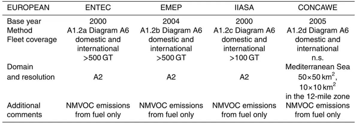
The regional European inventories, ENTEC (Whall et al. , 2002), EMEP (Vestreng et al., 2007), CONCAWE (2007) and IIASA (Cofala et al., 2007), all share the same spatial distribution and the same methodology and hence deliver comparable emission estimates for all compounds. The methodology applied here is a bottom-up approach 5

and it is based on the distance each ship covers, the information provided by the Lloyd’s Intelligence Unit (LMIU, 2004). Regional inventories give a much higher emission es-timate for the Mediterranean Sea for all compounds (except NMVOCs) as compared to the global inventories not only because of different methodologies but also due to the inclusion of domestic shipping in the regional inventories (Wang et al., 2008). The 10

ship emissions of NMVOC are most uncertain. In EDGAR a very low NMVOC emis-sion factor has been assumed (Appendix A) resulting in two orders of magnitude lower emissions as compared to all the other inventories. Only in Eyring the evaporation of hydrocarbons during loading and handling has been considered, making some 50% of the total NMVOC emissions, which explains the difference between Eyring and all 15

regional inventories.

One of the main advantages of the global inventories is their global coverage. Fur-thermore, the top-down approach used for global inventories allows a much faster emission calculation than the more detailed hence time consuming bottom-up ap-proach used by the regional inventories. On the other hand, the resolution of the 20

regional inventories is usually finer and their spatial distribution much more accurate. Since international fuel statistics do not include the fuel consumed for domestic ship traffic – from harbor to harbor within the same country – it has not been represented by the global inventories. The domestic ship tra_ffic can be significant for the inland seas like the Mediterranean, which is surrounded by 22 countries. Applying bottom-up ap-25

proach on a global scale would not only be much too costly, but would also be limited by the global unavailability of detailed ship movement data.

(7)

ACPD

9, 7155–7211, 2009

inventories?

E. Marmer et al.

Title Page

Tables Figures

◭ ◮

Back Close

Full Screen / Esc

Interactive Discussion using top-down approach like all the previous versions of EDGAR, but the calculation

takes into account 15 different vessel types and distinguishes between harbor and sea activities. Furthermore, it combines AMVER and ICOADS ship activity data sets (Wang et al., 2008) largely improving the spatial resolution from 1◦×1◦ to 0.1◦×0.1◦. Additionally to the international fuel statistics, the national fuel data is used to account 5

for the domestic ship traffic, its contribution ranging from 17–27% of total emissions, depending of different assumptions (Appendix A).

In all investigated inventories a temporally constant emission flux was assumed, i.e. the emissions are constant throughout the year. More details on methodology, distri-bution and coverage of different inventories can be found in Appendix A.

10

3 Modeling set-up

3.1 Ship emissions

For the model simulations in this study we have implemented the two global inventories (EDGAR and Eyring) and one regional inventory (EMEP) embedded into EDGAR on the global scale, to simulate the contribution of ship emissions to air pollution, attempt-15

ing to evaluate the inventories by comparing the simulated ozone and black carbon sur-face concentrations with measurements sampled onboard a cruise ship and at three coastal sites, and the simulated atmospheric NO₂ columns with those obtained from satellite data. For a more detailed evaluation we have separated the Mediterranean in 2 regions – the Eastern Mediterranean, referred to as EM (6 W to 15 E) and the West-20

ern Mediterranean, referred to as WM (16 E to 36 E). For the substances analyzed in this work, the NOx, NMVOCs and BC, the emissions for these areas are shown in

Ta-ble 2. It should be noticed, that the East-West distribution in EDGAR and Eyring is nearly 40/60 for all compounds, while in EMEP it is close to 50/50. This discrepancy is probably due to the domestic shipping which is not considered in the global inventories 25

(8)

ACPD

9, 7155–7211, 2009

inventories?

E. Marmer et al.

Title Page

Tables Figures

◭ ◮

Back Close

Full Screen / Esc

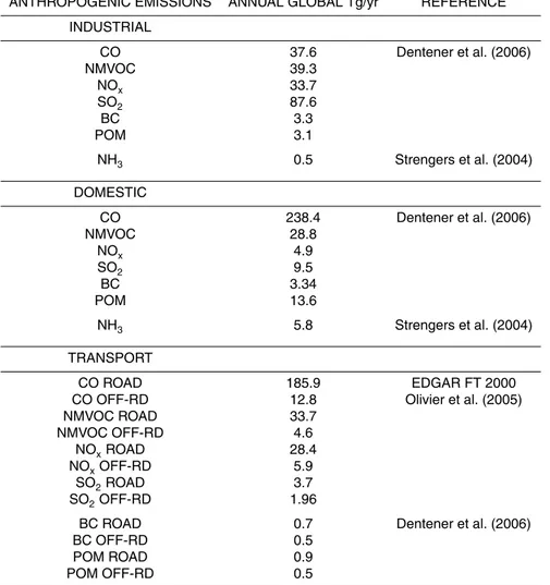
Interactive Discussion 3.2 Other emissions

Only ship emissions have been varied in the different model runs, all other emissions – natural and anthropogenic – have been kept unchanged. The emissions are summa-rized in Appendix B.

3.3 Chemistry transport model TM5 5

The TM5 is an off-line global transport chemistry model (Krol et al., 2005) and is driven by ECMWF ERA-40 reanalysis meteorological data. It has a spatial global resolution of 6◦×4◦and a two-way zooming algorithm that allows regions to be resolved at a finer resolution of 1◦×1◦. To smooth the transition between the global 6◦×4◦ region and the regional 1◦×1◦domain (Mediterranean Sea in the present application), a domain with a 10

3◦×2◦resolution (Northern Hemisphere in the present application) has been added. In the current version, the model has a vertical resolution of 34 layers, defined in a hybrid sigma-pressure coordinate system with a higher resolution in the boundary layer and around the tropopause. The height of the first layer is approximately 50 m.

The model transport has been extensively validated using 222Rn and SF6 (Peters 15

at al., 2004; Krol et al., 2005) and further validation was performed within the EVER-GREEN Project (Bergamaschi et al., 2006).

Gas phase chemistry is calculated using the CBM-IV chemical mechanism (Gery et al., 1989a,b) modified by Howeling et al. (1998), solved by means of the EBI method (Hertel et al., 1993). Dry deposition is calculated using the ECMWF surface character-20

istics and the resistance method (Ganzeveld and Lelieveld, 1995).

The aerosol compounds are considered only by mass and include sulfate, nitrate and ammonium, black and organic carbon, sea salt and dust. Black carbon is assumed to reside in the accumulation mode with a mass mean radius of 0.14µm for wet and dry

removal. In cloud-free model grid-cells BC is considered hydrophobic and does not 25

(9)

ACPD

9, 7155–7211, 2009

inventories?

E. Marmer et al.

Title Page

Tables Figures

◭ ◮

Back Close

Full Screen / Esc

Interactive Discussion We have performed six different model simulations (Table 3) for the meteorological

year 2006. In each simulation, all land based emissions have been kept unchanged (see Sect. 3.2). In order to calculate the impact of ship emissions on the atmospheric concentration, we have performed a simulation which did not include any ship emis-sions at all; this experiment is referred to as NON. Two global ship emission inventories 5

have been implemented, EDGAR FT 2000 – the simulation referred to as EDG – and Eyring – the simulation referred to as EYR. The regional EMEP ship emission inventory was selected for the forth experiment. Since we run our model on a global scale, this inventory was embedded into the global EDGAR ship emission inventory. We refer to this experiment as to EMEDG. In order to analyze the role of NMVOC from ships for the 10

surface ozone formation, we have run a sensitivity study with the same ship emissions as in EMEDG for all species but without any NMVOCs released from ships. This sensi-tivity experiment is referred to as EMEDG-noVOC. In all experiments described above, ship emissions have been released into the first vertical model layer and distributed between 0–30 m, while in real world ship stacks can reach as high as 50 m. In the 15

EMEDG H experiment we have tested the sensitivity towards the emission height by distributing all ship emissions between 30 and 100 m above surface. The global emis-sion inventories refer to the year 2000, EMEP refers to the year 2004, while the model simulations represent the year 2006. With an annual growth rate of 2.5% (Endresen et al., 2003), 16% more ship emissions would be released for EDGAR and Eyring, and 20

5% for EMEP in 2006. The resulting surface concentrations for BC and NO2 can be

easily calculated, but not for ozone due to non-linearity (see Sect. 4.2). This assump-tion would result in a 1.2% higher BC concentraassump-tion for the EMEDG simulaassump-tion, 1.3% for EDG and 0.4% for EYR. For NO2, the concentration would increase by 2.2% for the

EMEDG simulation, by 2.4% for EDG and by 5% for EYR. We did not correct for these 25

(10)

ACPD

9, 7155–7211, 2009

inventories?

E. Marmer et al.

Title Page

Tables Figures

◭ ◮

Back Close

Full Screen / Esc

4 Observations

4.1 Onboard ship observations

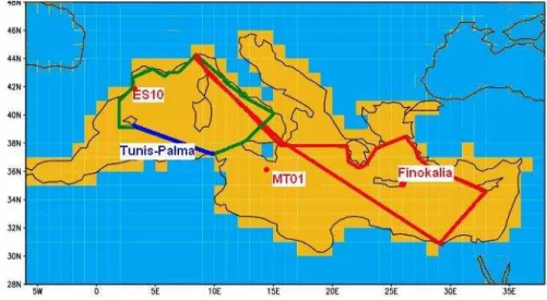
A set of monitoring instruments has been installed on board of a Mediterranean cruise ship Costa Fortuna with regular weekly routes in the Western Mediterranean during late spring, summer and fall and in the Eastern Mediterranean during winter (Velchev 5

et al., 2009, and Fig. 1). This campaign was launched in fall 2005 and is still on-going. Measurements of ozone, black carbon and the aerosol size distribution are performed every 10 min and the meteorological data are logged every 15 min.

The instruments are placed in a cabin at the front of the ship, 47 m above sea-level. Ozone is measured by a Thermo C49 ozone analyzer, equivalent BC was measured 10

by a 2-wavelength aethalometer from Magee Scientific (model AE 21). The stated pre-cision of the ozone analyzer is 1 ppbv, the observed zero-drift between calibrations was 1 ppbv and the span-drift was between 0 and 3%. Thus for the ozone concentrations measured over the Mediterranean Sea the typical uncertainty is approximately 2 ppbv. While the aethalometer measures black carbon as the attenuation of light divided 15

by an absorption cross section, the source characterization studies that form the basis of the emission inventories mainly rely on determinations of “elemental carbon” (Bond et al., 2004). Elemental carbon is determined by a thermo-optical method and de-fined operationally. Several studies show close to linear correlations between black carbon and elemental carbon concentrations, however the proportionally factor shows 20

large variations between di_fferent sampling sites (Jeong et al., 2004). The aethalome-ter measurements of BC on Costa Fortuna were carried out using the value of the absorption cross section provided by the manufacturer; the method was compared to thermo-optical determinations of elemental carbon during two campaigns; for aerosols over the sea, the methods were found to agree within a range of 25%.

25

(11)

ACPD

9, 7155–7211, 2009

inventories?

E. Marmer et al.

Title Page

Tables Figures

◭ ◮

Back Close

Full Screen / Esc

Interactive Discussion described by Cavalli et al. (2009). Most dust events took place during winter months

when the ship has been on cruise in the Eastern Mediterranean. This finding can be confirmed by the results from satellite observations (Papadimas at al., 2008) showing high frequency of dust events in the Eastern Mediterranean during winter.

Meteorological data (surface pressure and air temperature) were provided from the 5

automatic measurement station on the ship. Information on the position, speed and direction of the ship were available, identifying situations where contamination from the emissions of the ship itself might interfere with the measurements.

The cruise ship is mostly sailing during the evening/night and stays in harbors during the day; exceptions are the routes Tunis-Palma and Alexandria-Messina, where both 10

day and night hours are included. For our purpose we only consider the open sea measurements removing the data collected in harbors from 2 h prior to arrival to 2 h after the departure.

The TM5 model samples ozone, black carbon and the meteorological data every 30 min simultaneously with the cruise ship. We have compared the ozone and black 15

carbon measurements separately averaged over all Eastern and all Western cruises with the model results from each of the experiments.

4.2 Satellite measurements

The OMI instrument is a nadir viewing imaging spectrograph that measures the solar radiation backscattered by the Earth’s atmosphere and surface over the entire wave-20

length range from 270 to 500 nm with a spectral resolution of about 0.5 nm. The 114◦ viewing angle of the telescope corresponds to a 2600 km wide swath on the surface, which enables measurements with a daily global coverage (Boersma et al., 2007). The error of a single OMI retrieval is best referred to as 1.0×1015molecules cm−2+30%, for detailed error analysis please see Boersma et al. (2004, 2007). The TM5 has sam-25

pled the NO2atmospheric column simultaneously with the satellite overpass at 13:30 h

(12)

ACPD

9, 7155–7211, 2009

inventories?

E. Marmer et al.

Title Page

Tables Figures

◭ ◮

Back Close

Full Screen / Esc

Interactive Discussion grid to be covered by OMI data. The grid boxes not meeting this criterion were marked

as cloudy and filtered. The same grid boxes were also filtered from the TM5 samples as well to assure better comparability. Thus if OMI has seen more than 50% of the grid box as “cloudy”, this grid box has been excluded from the evaluation, because the clouds screen the NO2 below, which can not be retrieved. For statistical significance

5

only summertime observations have been taken into account, when cloud free condi-tions prevail. The monthly mean NO₂columns for June, July and August 2006 resulting from the experiments NON, EDG, EYR and EMEDG have been compared with satellite measurements.

5 Results

10

All comparisons with observational data show that the TM5 model can simulate the level of air pollutants over the Mediterranean Sea reasonably well.

5.1 Black carbon

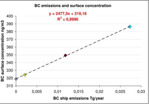
In this version of TM5 black carbon is treated as bulk mass, e.g. we do not consider par-ticle size and number distribution. Black carbon does not participate in chemical reac-15

tions, once emitted it is advected by turbulence and large scale eddies and is removed by dry and wet deposition, thus acting as a passive tracer. Therefore we expect a linear model response of black carbon surface concentration to varying emissions (Fig. 2). Releasing the emissions at higher levels 30–100 m as in the experiment EMEDG-H rather than 0–30 m reduces the mean surface concentration by 3.6%. This difference 20

(13)

ACPD

9, 7155–7211, 2009

inventories?

E. Marmer et al.

Title Page

Tables Figures

◭ ◮

Back Close

Full Screen / Esc

Interactive Discussion tion with highest BC emissions, the contribution is 35–50% close to the main shipping

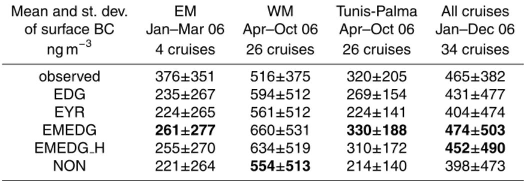
routes in the Eastern and the Western part, about 15–25% over large distances over the North African coast during summer, while at the Southern European coast the con-tribution is less than 15%. Comparison of the mean measurements obtained during all Eastern and all Western cruises with the mean of simultaneously sampled model BC 5

concentrations shows a slight overestimation of the simulated BC of the cruises in the WM (April to October, Table 4). Even the simulation without ships gives a higher BC concentration than the observed one indicating too high emissions from land based sources in the model. If we look separately at the results for the leg Tunis-Palma de Mallorca (TP, Fig. 1), which crosses the highly frequented shipping route at 37 N, the 10

agreement largely improves and we find the best agreement with EMEDG (Table 4). In vicinity of the emission sources, the properties of black carbon correspond better to those assigned to it in the model, before internal mixing with other particles and aging can have an a_ffect on its hydroscopicity and wet deposition. The underprediction of BC during the EM winter cruises (January to March) could result from too high deposition 15

of BC in the model. There is a pronounced annual cycle in the simulated BC surface concentration with a maximum in July and a minimum in March. To a great extend the annual cycle in the model is driven by precipitation and wet deposition of BC (Fig. 4). It is difficult to conclude about the BC annual cycle over the Mediterranean based on the on-board measurements, since the ship travels in di_fferent regions during the di_fferent 20

seasons, but from the BC measured at Finokalia, a site on Crete Island in the Eastern Mediterranean, no pronounced annual cycle could be detected. A comparison of BC observations at this site with model simulations shows that during winter, the surface BC is underestimated by the model, while it is overestimated during summer (Fig. 5). Looking at the average value for all cruises, the EMEDG simulation provides the best 25

(14)

ACPD

9, 7155–7211, 2009

inventories?

E. Marmer et al.

Title Page

Tables Figures

◭ ◮

Back Close

Full Screen / Esc

Interactive Discussion 5.2 Ozone

Ship emissions contribute to a much lesser degree to the surface ozone as compared to BC. During the summer 2006, this contribution reached 2–4% over the Sea in EDG. The maximum contribution of 12% (EYR simulation) can be found in summer over the Strait of Gibraltar, which links the Mediterranean Sea to the North Atlantic Ocean 5

(Fig. 6). The relation between the emissions of the precursor gases NO_x (NO2+NO) and NMVOCs, and surface ozone is highly non linear: Linearity can be found between the NOx emissions and the NO2 concentration levels (Fig. 7). The relation between

the NO_x emissions and the surface ozone is not that simple: initially, increase of NO_x emissions results in an enhanced surface ozone concentration, in the EMEDG simu-10

lation, however, we find lower surface ozone as compared to EYR despite higher NOx

emissions (Fig. 8). Our analysis shows that when the threshold value of 1.2 Tg year−1 NO_x emissions is exceeded, the surface ozone goes down. In this analysis we need to consider the impact of hydrocarbons, which show a highly non-linear behavior. In the NON simulation, without any emissions over the Mediterranean, we find the high-15

est mean NMVOC surface concentration of all simulations, 17.8 ppbv(C). From NON to EMEDG-noVOC we have added ship emissions of all the components except of the NMVOCs, only to find the lowest mean NMVOC concentration of all simulations, 17.2 ppbv(C). Despite the fact that the VOC ship emissions are either zerro (in NON and EMEDG-noVOC) or differ by over two orders of magnitude (between EDG and 20

EYR), their effect on the surface concentration ranges only within 3%. Our analysis of the very complicated photochemical patterns between NO_x, NMVOCs and ozone shows a relationship between the NMVOC/NOxratio and the ratio of ozone production

rate to the ozone loss rate (Fig. 9). At low NMVOC/NOxratios the relation of ozone

pro-duction to ozone loss remains low and it grows with the growing ratio. After reaching 25

the maximum at a threshold ratio of NMVOC/NOx=8, it begins to decrease. Because of this very high sensitivity of ozone levels to the emissions of NOx and especially

(15)

emis-ACPD

9, 7155–7211, 2009

inventories?

E. Marmer et al.

Title Page

Tables Figures

◭ ◮

Back Close

Full Screen / Esc

Interactive Discussion sions is essential in order to study and understand their possible impact on the ozone

levels especially in such polluted areas as the Mediterranean Sea.

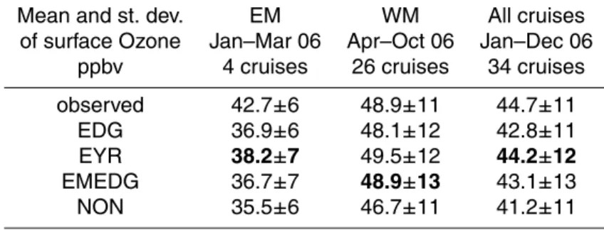
In terms of ozone measurements, the best agreement is achieved over the WM dur-ing the “summer” (April to October) cruises. The observed mean ozone of 48.9 ppbv is best simulated in EMEDG, the EYR simulation gives slightly higher value and EDG 5

slightly lower. Without ship emissions, the simulated mean ozone over the WM de-creases by 2 ppbv (Table 5). Much higher mean value has been observed (42.7 ppbv) during the EM cruises (January–March) than the model predicts (maximal simulated value 38.2 ppbv in EYR). Lelieveld et al. (2002) and Gerasoupoulos et al. (2005) identi-fied transport from the European continent as the main mechanism that controls ozone 10

levels in the Eastern Mediterranean. Therefore we can not simply translate this un-derestimation into the shortcomings of the local emissions. Inaccuracy in land based emissions of the ozone precursors; simulated vertical mixing and transport could be additional sources of uncertainty. Averaged over all cruises, Eyring inventory presents the bests results. Figure 10a, b shows the comparison with observations at three 15

coastal sites (Fig. 1), averaged over the same time period as the Eastern (1 January–3 March 2006) and the Western (26 April–31 October) cruises. At the western Mediter-ranean site Cabo de Creus (ES10) (Fjaeraa and Hjellbrekke, 2008) and the eastern Mediterranean site Finokalia, the model performs better during summer than during winter. During summer, EYR simulation gives the best agreement for Cabo de Creus, 20

in agreement with the results for the WM cruises. For Finokalia the summertime ozone is best simulated with EMEDG.

At the central Mediterranean site Giordan Lighthouse (MT01) (Fjaeraa and Hjell-brekke, 2008) the summertime surface ozone is overestimated by all simulations. Dur-ing winter we find an underestimation by all simulations at all three sites. Seasonal 25

(16)

ACPD

9, 7155–7211, 2009

inventories?

E. Marmer et al.

Title Page

Tables Figures

◭ ◮

Back Close

Full Screen / Esc

Interactive Discussion 5.3 NO₂column burden

The advantage of satellite measurements for validation of ship emission inventories is their spatial coverage. As compared to the ship observations we have a good coverage of continuous measurements which enables us to compute mean values over reason-ably long time period. What we can observe from the satellite is the total atmospheric 5

burden rather than the surface concentration which might let us wonder whether such local surface sources as ships can leave a signal on these observations. From the OMI satellite picture a weak but significant signal from the main ship route crossing the Mediterranean Sea is clearly recognizable (Fig. 11a). In order to make the data comparable to the model results, we interpolate it from the original resolution of OMI 10

(see Sect. 4.2) to the model resolution of 1◦×1◦. This interpolation causes a smearing of the signal and it nearly disappears over the Eastern part of the Sea but can still be well recognized in the Western part (Fig. 11b). The total atmospheric NO2burden over

the Mediterranean Sea is overpredicted by the model, the NON simulation gives the best quantitative agreement with the satellite observations (Table 6). We compare the 15

burden over the particular area of the main shipping routes in the Eastern and Western Mediterranean as can be seen from space (Fig. 12). While for the Eastern part EDG, the simulation with lowest NOxemissions, gives the best results for the summer mean

NO₂ burden, it is significantly higher over the Western Mediterranean, and is best re-produced by the EMEDG simulation. For the Western Mediterranean we find a good 20

agreement with measurements for both, NO2 and ozone, and in both cases it is the

EMEDG simulation that produces best matching results.

6 Conclusions and discussion

All ship emission inventories analyzed here give different estimates for all compounds; these disagreements mainly result from di_fferent methodologies, activity data and emis-25

(17)

ACPD

9, 7155–7211, 2009

inventories?

E. Marmer et al.

Title Page

Tables Figures

◭ ◮

Back Close

Full Screen / Esc

Interactive Discussion carbon, which vary by a factor of 5, and even more for NMVOCs which vary by two

orders of magnitude. Emission factors for NOxand SO2agree much better among the

inventories. Furthermore, the global inventories apply international bunker statistics, in which the fuel consumed for the domestic shipping is not included. The national fuel statistics have been taken into account in the new EDGARv4 inventory, but the spatial 5

information for the domestic shipping has not yet been provided. Comparing the emis-sion totals we find that at least 20% of the emisemis-sions in the Mediterranean account for the domestic traffic. All regional inventories are based on individual ship movements, providing a better fleet coverage, but this information is not available on a global scale, thus this method can not be applied globally. Seasonal variability of ship traffic has not 10

been included in any of the inventories; all emissions are assumed temporally constant which presents an additional uncertainty.

So what did we learn from the measurements about the ship emission inventories? We can say with a relative certainty, that ship emissions have a significant impact on air pollution over the Mediterranean region. The evidence for this impact is the ship signal 15

which is recognizable from the satellite NO2 retrievals especially over the Western

Mediterranean. Over the Eastern Mediterranean, we find a spatially narrow signal in the satellite NO2retrievals which is not reproducible by 1◦×1◦resolution applied in this

study. With EDGARv4, we now have a much finer resolved emission inventory which should be applied in a model with a corresponding 0.1◦×0.1◦resolution in future. 20

We can divide our results in four categories – Western Mediterranean summer, West-ern Mediterranean winter, EastWest-ern Mediterranean summer and EastWest-ern Mediterranean winter. We compare NO₂ satellite retrievals for Eastern and Western Mediterranean summer (June, July and August). The ship measurements of ozone and black car-bon are available for the Western Mediterranean summer (April to October) and the 25

(18)

ACPD

9, 7155–7211, 2009

inventories?

E. Marmer et al.

Title Page

Tables Figures

◭ ◮

Back Close

Full Screen / Esc

Interactive Discussion For all pollutants, we find the best agreement between the model and the

obser-vations in the WM during the dry summer. For NO₂, EMEP, emission inventory with highest NOx emissions, produces best results in the Western Mediterranean which is

corroborated by the good agreement of EMEDG (the corresponding simulation) ozone with measurements during Western cruises. For the western observational site Cabo 5

de Cruise it is the EYR simulation (Eyring inventory) which agrees best with the ob-served ozone. Simulated ozone concentrations for EMEP and Eyring emission inven-tories are very similar. While 1.8 times more NO_xis released in EMEP than in Eyring in the Western part, 2.6 more NMVOCs are released in Eyring than in EMEP. Due to com-plicated non linear photochemistry and the sensitive relationship of NOx, NMVOCs and

10

ozone, we are unable to give preference to one of these inventories based on ozone and NO2measurements only. Ship stack measurements of NMVOCs in order to better

determine the emission factor for this group of compounds can greatly contribute to the improvement of NMVOC ship emission estimates. Furthermore we recommend mea-suring NMVOC on-board the cruise ship along with ozone and NOx(the NOx analyzer

15

has been installed on board in 2008). Better knowledge of the NMVOC emissions and ambient concentrations over the sea can improve our knowledge on the impact of ship emissions on surface ozone. Black carbon is slightly overestimated during the Western cruises, as well as at the eastern site Finokalia during the dry season. Even without ship emissions, the simulated BC concentration exceeds the observed one on average. 20

For the Tunis-Palma leg, which is largely dominated by local ship emissions there is a very good agreement with simulated BC, also here the best results are achieved with EMEP.

The emissions in the Eastern Mediterranean are not constraint with the measure-ments used in this study. During the EM summer, very low NO2 has been observed

25

(19)

ACPD

9, 7155–7211, 2009

inventories?

E. Marmer et al.

Title Page

Tables Figures

◭ ◮

Back Close

Full Screen / Esc

Interactive Discussion Eastern part – either the model deposits too much BC by the wet deposition, or it could

be attributed to missing emission sources – marine or land – during winter. Incorrect temporal variability of BC land sources like biomass burning could be the reason for the slight overestimation during summer and the underestimation during winter.

All ship emission inventories analyzed in this work are assumed to be temporally 5

constant. In this study, summertime simulations of all compounds have shown bet-ter agreement with measurements as compared to winbet-ter. Different seasonal patterns are given by global ship activity data sets ICOADS and AMVER and need more in-vestigation (Dalsøren et al., 2008). Including the temporal variability in ship emission inventories could possibly improve the simulations of ozone and BC during winter. 10

Considering the uncertainties in the measurements and the model, we can say that all ship emission estimates lay within the uncertainty range. While more stack mea-surements and detailed fleet statistics can further improve our knowledge on ship emis-sions, the di_fficulty to construct an accurate emission estimate will remain a challenge for this highly uncertain emission source. Given the expected growth of ship traffic and 15

the expansion of waterways and ports, scenario calculations are needed to determine the impact of emission reduction policies on air quality and climate. For these cal-culations, the whole range of existing inventories needs to be considered in order to determine the propagation of these uncertainties in the future scenarios.

Appendix A

20

Ship emission inventories – methodologies and emission factors

Global and European regional inventories are calculated based on di_fferent method-ologies.

Global emission inventories are calculated applying the top-down approach. Top-25

(20)

ACPD

9, 7155–7211, 2009

inventories?

E. Marmer et al.

Title Page

Tables Figures

◭ ◮

Back Close

Full Screen / Esc

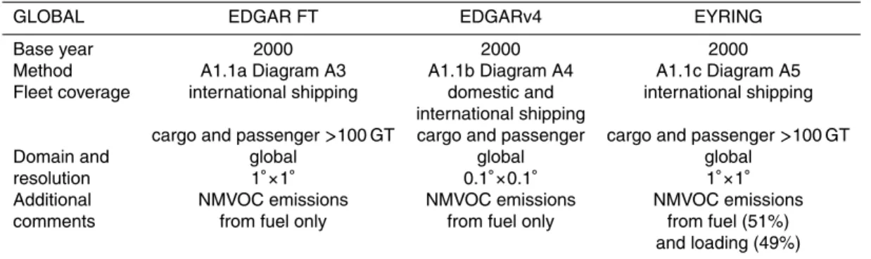
Interactive Discussion on the total fuel consumption. Geo-spatial information is not included here. The total

fuel consumption is either based on energy statistics data (classical top-down, EDGAR FT, Diagram A3) or estimated from the fleet activity (activity based top-down, Eyring, Diagram A5). The new EDGARv4 inventory (Diagram A4) applies a technology split accounting for different ship types and sea and port activities. The calculated global 5

ship emissions total is allocated to each grid cell proportional to the value of each grid represented by spatial proxies of the ship activity patterns from the AMVER (Auto-mated Mutual-Assistance Vessel Rescue System) data set (Endresen et al., 2003) or on the combined AMVER/ICOADS (International Comprehensive Ocean-Atmosphere Data Set) data (Wang et al., 2008).

10

In regional inventories, the up approach is applied (Diagram A6). In a bottom-up approach the individual base elements of the system are first specified in great detail. These elements are then linked together to form the main system. Thus, the emissions are calculated based on information from individual vessels and its move-ments.

15

A1 Methods

A1.1 Top-down (Table A1a)

Based on fuel consumption.

(a) Bunker fuel statistics provided by the International Energy Agency (IEA), spa-tial distribution based on AMVER Ship Reporting System Data (Endresen et al., 20

2003).

(b) Bunker fuel statistics privided by IEA and national fuel statistics to account for the domestic ship traffic, spatial distribution based on combined AMVER/ICOADS activity data (Wang et al., 2008).

(c) Activity based – total fuel consumption based on fleet activity data, spatial distri-25

(21)

ACPD

9, 7155–7211, 2009

inventories?

E. Marmer et al.

Title Page

Tables Figures

◭ ◮

Back Close

Full Screen / Esc

Interactive Discussion A1.2 Bottom-up (Table A1b)

Emissions calculated by engine type/engine speed/fuel type and vessel movements, for vessels>500 GT, data on vessel characteristics provided by Lloyd’s Register Fairplay

(LRF, 2004) . Top-down approach for smaller vessels and fishing vessels.

(a) Provided by Lloyd’s Marine Intelligence Unit (LMIU, 2004) for four discrete months 5

in 2000 to reflect seasonal variations in shipping activity, the results multiplied by 3. In-port times derived from a questionnaire survey of ports. Separate analysis for ferries and fishing vessels.

(b) Based on (a), assuming a growth factor of 2.5% per year (Endresen et al., 2003).

(c) Same as (a), using additional literature data on port surveys, resulting in an in-10

crease of 20% in average port times as compared to (a). Top-down approach for smaller (100–500 GT) vessels, assuming additional 10% of emissions in the coastal 12-mile zones. More detailed spatial resolution of emissions, distinguish-ing national, international, by flag state and within 12-mile zones.

(d) Same as (a), but up-dated for 2005, manual addition of approx. 100 000 passen-15

ger vessel movements using time tables. Different methodology for determining the relative percentages of RO (residual oil) and MD (marine diesel) in total fuel consumed.

A2 EMEP domain and resolution (Table A1b)

Approx. 40 W–60 E lat, 30 N–90 N lon, North-East Atlantic, North, Baltic, Black and 20

(22)

ACPD

9, 7155–7211, 2009

inventories?

E. Marmer et al.

Title Page

Tables Figures

◭ ◮

Back Close

Full Screen / Esc

(23)

ACPD

9, 7155–7211, 2009

inventories?

E. Marmer et al.

Title Page

Tables Figures

◭ ◮

Back Close

Full Screen / Esc

(24)

ACPD

9, 7155–7211, 2009

inventories?

E. Marmer et al.

Title Page

Tables Figures

◭ ◮

Back Close

Full Screen / Esc

Interactive Discussion A4.1 Domestic navigation in EDGARv4

Some of the fuel being used at open sea is related to inland transportation for exam-ple from one harbor to another harbor in the same country. This fuel is excluded from the IEA statistics on international bunker fuel but included in national bunker statistics. Globally, the variety of ship types in domestic navigation is large and is dependent on 5

the geography of countries. For most countries no detailed split between vessel types and amount of fuel consumed is available. As first estimate until better statistics be-come available all domestic fuel consumption has been assigned to freight traffic with emission factors according to Dalsøren et al. (2008). Furthermore, in the region of interest, we do not know to what extend the fuel has been consumed in the Mediter-10

(25)

ACPD

9, 7155–7211, 2009

inventories?

E. Marmer et al.

Title Page

Tables Figures

◭ ◮

Back Close

Full Screen / Esc

(26)

ACPD

9, 7155–7211, 2009

inventories?

E. Marmer et al.

Title Page

Tables Figures

◭ ◮

Back Close

Full Screen / Esc

(27)

ACPD

9, 7155–7211, 2009

inventories?

E. Marmer et al.

Title Page

Tables Figures

◭ ◮

Back Close

Full Screen / Esc

Appendix B

Other emissions

Only ship emissions have been varied for the di_fferent model simulations. All other emissions have been kept the same for all simulations (Tables B1–B3).

5

Acknowledgements. This study was partially supported by the EU project MAP (Marine Aerosol

Production). We thank Veronika Eyring and Vigdis Vestreng for providing information on their emission inventories. The work has also been inspired by participation in the Harbours, Air Quality and Climate Change conference in Rotterdam 2008.

References

10

ARB (Air Resources Board): Emission Reduction Plan from Ports and Goods Movement, Cali-fornia Environmental Protection Agency, 21 June 2006, Los Angeles, USA, 2006. 7157 Andersson-Skøld, Y. and Simpson, D.: Secondary organic aerosol formation in Northern

Eu-rope: a model study, J. Geophys. Res., 106, 7357–7374, 2001. 7159

Andres, R. and Kasgnoc, A.: A time-averaged inventory of aerial volcanic sulfur emissions, J.

15

Geophys. Res., 103, 25251–25261, 1998. 7197

Bergamaschi, P., Meirink, J. F., M ¨uller, J. F., K ¨orner, S., Heimann, M., Bousquet, P.,. Dlugo-kencky, E.J, Kaminski, U., Vecchi, R., Marcazzan, G., Meinhardt, F., Ramonet, M., Sartorius, H., and W. Zahorowski: Model Inter-comparison on Transport and Chemistry – report on model inter-comparison performed within European Commission FP5 project EVERGREEN

20

Report EUR 22241 EN, 53, 4–48, 2006. 7162

Boersma, K. F., Eskes, H. J., and Brinksma, E. J.: Error analysis for tropospheric NO₂retrieval from space, J. Geophys. Res., 109, D04311, doi:10.1029/2003JD003962, 2004. 7165 Boersma, K. F., Eskes, H. J., Veefkind, J. P., Brinksma, E. J., van der A, R. J., Sneep, M., van

den Oord, G. H. J., Levelt, P. F., Stammes, P., Gleason, J. F., and Bucsela, E. J.: Near-real

25

(28)

ACPD

9, 7155–7211, 2009

inventories?

E. Marmer et al.

Title Page Abstract Introduction Conclusions References Tables Figures ◭ ◮ ◭ ◮ Back Close

Full Screen / Esc

Bond, T., Streets, D., Yarber, K., Nelson, S., Woo, J., and Klimont, Z.: A technology-based global inventory of black and organic carbon emissions from combustion, J. Geophys. Res., 109, D14203, doi:10.1029/2003JD003697, 2004. 7159, 7164

Bouwman, A. F., Lee, D. S., Asman, W. A. H., Dentener, F. J., van der Hoek, K. W., and Olivier, J. G. J.: A global high-resolution emission inventory for ammonia, Global Biogeochem. Cy.,

5

11, 561–578, 1997. 7197

Cavalli, F., Vignati, E., Velchev, K., Hjorth, J., Dell’Acqua, A., Schembari, C., and Marmer, E.: Black carbon over the Mediterranean Sea – results from two year fo shipborne measurments, in preparation, 2009. 7165

Clean Air For Europe: Impact Assessment, online available at: http://ec.europa.eu/

10

environment/air/cafe/pdf/ia report en050921 final.pdf, p. 31, last access: February 2009, 2005. 7157

Cofala, J., Amann, M., Hezes, C., Wagner, F., Klimont, Z., Posch, M., Sch ¨opp, W., Tarasson, L., Eiof Jonson, J., Whall, C., and A. Stavrakaki: Analysis of Policy Measures to Reduce Ship Emissions in the Context of the Revision of the National Emissions Ceilings Directiv, Final

15

Report, Submitted to the European Commission, DG Environment, Unit ENV/C1, Contract No 070501/2005/419589/MAR/C1, IIASA Contract No. 06-107, 2007. 7157, 7160

Concawe: Ship Emissions Inventory-Mediterranean Sea, Final Report, April 2007, Entec UK Limited, 47 pp., 2007. 7160

Corbett, J. J., Winebrake, J. J., Green, E. H., Kasibhatla, P., Eyring, V., and Lauer, A.: Mortality

20

from Ship Emissions: A Global Assessment, Environ. Sci., Technol., 41(24), 8512–8518, doi:10.1021/es071686z, 2007a. 7157

Dalsøren, S. B., Eide, M. S., Endresen, Ø., Mjelde, A., Gravir, G., and Isaksen, I. S. A.: Update on emissions and environmental impacts from the international fleet of ships. The contribu-tion from major ship types and ports, Atmos. Chem. Phys. Discuss., 8, 18323–18384, 2008,

25

http://www.atmos-chem-phys-discuss.net/8/18323/2008/. 7173, 7178

Deniz, C. and Durmuso ˆglu, Y.: Estimating shipping emissions in the region of the Sea of Mar-mara, Turkey, Sci. Total Environ., 390(1), 255–261, 2008. 7158

Derwent, R., Stevenson, D. S., Doherty, R. M, Collins, W. J., Sanderson, M. G., Amann, M., and Dentener, F.: The contribution from ship emissions to air quality and acid deposition in

30

Europe, Ambio, 34, 54–59, 2005. 7157

(29)

ACPD

9, 7155–7211, 2009

inventories?

E. Marmer et al.

Full Screen / Esc

Endresen, Ø., Sørgard, E., Sundet, J., Dalsøren, S., Isaksen, I., Berglen, T., and Gravir, G.: Emissions from international sea transport and environmental impact,J. Geophys. Res., 108, 4560, doi:10.1029/2002JD002898, 2003. 7159, 7163, 7174, 7175

Eyring, V., Koehler, H. W., van Aardenne, J., and Lauer, A.: Emissions from in-ternational shipping: 1. The last 50 years, J. Geophys. Res., 110(D17), D17305,

5

doi:10.1029/2004JD005619, 2005. 7156, 7157, 7158, 7159, 7190

Eyring, V., Stevenson, D. S., Lauer, A., Dentener, F. J., Butler, T., Collins, W. J., Ellingsen, K., Gauss, M., Hauglustaine, D. A., Isaksen, I. S. A., Lawrence, M. G., Richter, A., Rodriguez, J. M., Sanderson, M., Strahan, S. E., Sudo, K., Szopa, S., van Noije, T. P. C., and Wild, O.: Multi-model simulations of the impact of international shipping on Atmospheric Chemistry

10

and Climate in 2000 and 2030, Atmos. Chem. Phys., 7, 757–780, 2007, http://www.atmos-chem-phys.net/7/757/2007/. 7157

Fjaeraa, A. M. and Hjellbrekke, A.-G.: Ozone measurements 2006, EMEP/CCC-Report 2/2008, EMEP (European Monitoring and Evaluation Programme), Kjeller, Norwegian Institute for Air Research, Norway, online available at: http://tarantula.nilu.no/projects/ccc/emepdata.html,

15

last access: 10 January 2008, 2008. 7169

Ganzeveld, L. and Lelieveld, J.: Dry deposition parameterization in a chemistry general circu-lation model and its influence on the distribution of reactive trace gases, J. Geophys. Res., 100, 20999–921012, 1995. 7162

Gerasopoulos, E., Kouvarakis, G., Vrekoussis, M., Kanakidou, M., and Mihalopoulos, N.:

20

Ozone variability in the marine boundary layer of the eastern Mediterranean based on 7-year observations, J. Geophys. Res., 110, D15309, doi:10.1029/2005JD005991, 2005. 7169 Gery, M. W., Whitten, G. Z., and Killus, J. P.: Development and testing of the CBM-IV for urban

and regional modelling, US EPA, Research Triangle Park EPA-600/3-88-012, 1989a. 7162 Gery, M. W., Whitten, G. Z., Killus, J. P., and Dodge, M. C.: A photochemical kinetics

mecha-25

nism for urban and regional scale computer modeling, J. Geophys. Res., 94, 12925–12956, 1989b. 7162

Ginoux , P., Chin, M., Tegen, I., Prospero, J. M., Holben, B., Dubovik, O., and Lin, S.-J.: Sources and distributions of dust aerosols simulated with the GOCART model, J. Geophys. Res., 106(D17), 20255–20273, 2001. 7197

30

(30)

ACPD

9, 7155–7211, 2009

inventories?

E. Marmer et al.

Full Screen / Esc

Gong, S. L., Barrie, L. A., Blanchet, J. P., von Salzen, K., Lohmann, U., Lesins, G., Spacek, L., Zhang, L. M., Girard, E., Lin, H., Leaitch, R., Leighton, H., Chylek, P., and Huang, P.: Canadian Aerosol Module: A size-segregated simulation of atmospheric aerosol processes for climate and air quality models 1. Module development, J. Geophys. Res.-Atmos., 108, 4007, doi:10.1029/2001JD002002, 2003. 7197

5

Granier, C., Niemeier, U., Jungclaus, J. H., Emmons, L., Hess, P., Lamarque, J. F., Walters, S., and Brasseur, G. P.: Ozone Pollution from Future Ship Traffic in the Arctic Northern Passages, Geophys. Res. Lett., L13807, doi:10.1029/2006GL026180, 2006. 7157

Guenther, A., Hewitt, C. N., Erickson, D., Fall, R., Geron, C., Graedel, T., Harley, P., Klinger, L., Lerdau, M., McKay, W., Pierce, T., Scholes, B., Steinbrecher, R. Tallamraju, R., Taylor,

10

J., and Zimmerman, P.: A global model of natural volatile organic compound emissions, J. Geophys. Res., 100, 8873–8892, 1995. 7197

Dentener, F., Kinne, S., Bond, T., Boucher, O., Cofala, J., Generoso, S., Ginoux, P., Gong, S., Hoelzemann, J. J., Ito, A., Marelli, L., Penner, J. E., Putaud, J.-P., Textor, C., Schulz, M., van der Werf, G. R., and Wilson, J.: Emissions of primary aerosol and precursor gases in

15

the years 2000 and 1750 prescribed data-sets for AeroCom, Atmos. Chem. Phys., 6, 4321– 4344, 2006,

http://www.atmos-chem-phys.net/6/4321/2006/. 7198

Halmer, M. M. and Schmincke, H.-U.: VGIS (Volcanic Gas Input into the Stratosphere), AGU 2000 Fall Meeting, 15–19 December, 2000, San Francisco, California, USA, 2000. 7197

20

Halmer, M. M., Schmincke, H.-U., and Graf, H. F.: The annual volcanic gas input into the atmosphere, in particular into the stratosphere: a global data set for the past 100 years, J. Volcanol. Geoth. Res., 115, 511–528, 2002. 7197

Hertel, O., Berkowicz, R., Christensen, J., and Hov, O.: Test of two numerical schemes for use in atmospheric transport-chemistry models, Atmos. Environ., 27, 2591–2611, 1993. 7162

25

Houweling, S., Dentener, F., and Lelieveld, J.: The impact of nonmethane hydrocarbon com-pounds on tropospheric photochemistry, J. Geophys. Res., 103, 10673–10696, 1998. 7162 IMO: IMO Newsroom, Press Briefings, Briefing 46, 10/10/2008, online available at: http://www.

imo.org/Newsroom/mainframe.asp?topic id₌1709\&doc id₌10262, 2008. 7157

Jeong, C. H., Hopke, P. K., Kim, E., and Lee, D. W.: The comparison between thermal-optical

30

transmittance elemental carbon and Aethalometer black carbon measured at multiple moni-toring sites, Atmos. Environ., 38, 5193–5204, 2004. 7164

(31)

ACPD

9, 7155–7211, 2009

inventories?

E. Marmer et al.

Full Screen / Esc

surface regional background ozone over Crete Island in the southeast Mediterranean, J. Geophys. Res., 105(D4), 4399–4407, 2000. 7158

Krol, M., Houweling, S., Bregman, B., van den Broek, M., Segers, A., van Velthoven, P., Peters, W., Dentener, F., and Bergamaschi, P.: The two-way nested global chemistry-transport zoom model TM5: algorithm and applications, Atmos. Chem. Phys., 5, 417–432, 2005,

5

http://www.atmos-chem-phys.net/5/417/2005/. 7158, 7162

Lack, D., Lerner, B., Granier, C., Baynard, T., Lovejoy, E., Massoli, P., Ravishankara, A. R., and Williams, E.: Light absorbing carbon emissions from commercial shipping, Geophys. Res. Lett., 35, L13815, doi:10.1029/2008GL033906, 2008. 7157, 7159

Lauer, A., Eyring, V., Hendricks, J., Jckel, P., and Lohmann, U.: Global model simulations of the

10

impact of ocean-going ships on aerosols, clouds, and the radiation budget, Atmos. Chem. Phys., 7, 5061–5079, 2007,

http://www.atmos-chem-phys.net/7/5061/2007/. 7157

Lelieveld, J. and Dentener, F. J.: What controls tropospheric ozone?, J. Geophys. Res., 105(D3), 3531–3551, 2000. 7158

15

Lelieveld, J., Berresheim, H., Borrmann, S., Crutzen, P. J., Dentener, F. J., Fischer, H., Fe-ichter, J.,Flatau, P. J., Heland, J., Holzinger, R., Korrmann, R., Lawrence, M. G., Levin, Z., Markowicz, K. M., Mihalopoulos, N., Minikin, A., Ramanathan, V., De Reus, M., Roelofs, G. J., Scheeren, H. A., Sciare, J., Schlager, H., Schultz, M., Siegmund, P., Steil, B., Stephanou, E. G., Stier, P., Traub, M., Warneke, C., Williams, J., and Ziereis, H.: Global air pollution

20

crossroads over the Mediterranean, Science, 298, 5594, 794–799, 2002. 7169

Lloyd’s Register of Shipping, London, Marine exhaust Emissions Quantification Study for the Mediterranean Sea, 1999. 7159

LMIU (Lloyd’s Marine Intelligence Unit): Extract from the vessel movement database 1999 (January, April, July and October), 2000. 7160, 7175

25

LRF, Lloyd’s Register Fairplay: Extract from the world fleet database (all civil ocean-going cargo and passenger ships above or equal to 100 GT), Redhill, UK, 2004. 7175

Marmer, E. and Langmann, B.: Impact of ship emissions on Mediterranean summertime pollu-tion and climate: A regional model study, Atmos. Environ., 39, 4659–4669, 2005. 7158 Olivier, J. G. J., Van Aardenne, J. A., Dentener, F., Pagliari, V., Ganzeveld, L. N., and

Pe-30

(32)

ACPD

9, 7155–7211, 2009

inventories?

E. Marmer et al.

Full Screen / Esc

Papadimas, C. D., Hatzianastassiou, N., Mihalopoulos, N., Querol, X., and Vardavas, I.: Spatial and temporal variability in aerosol properties over the Mediterranean basin based on 6-year (2000–2006) MODIS data, J. Geophys. Res.-Atmos., 113 , D11205, doi:10.1029/2007JD009189, 2008. 7165

Peters, W., Krol, M. C., Dlugokencky, E. J., Dentener, F. J., Bergamaschi, P., Dutton, G.,

5

Velthoven, P. V., Miller, J. B., Bruhwiler, L., and Tans, P. P.: Toward regional-scale model-ing usmodel-ing the two-way nested global model TM5: Characterization of transport usmodel-ing SF6, J. Geophys. Res.-Atmos., 109, D19314, doi:10.1029/2004JD005020, 2004. 7162

Sinha, P., Hobbs, P. V., Yokelson, R. J., Christian, T. J., Kirchstetter, T. W., and Bruintjes, R.: Emission of trace gases and particles from two ships in the southern Atlantic Ocean, Atmos.

10

Environ., 37, 2139–2148, 2003. 7159

Stern, N.: Stern Review on the Economics of Climate Change, HM Treasury, The Stationary O_ffice, London, 2007. 7157

Streets, D. G., Carmichael, G. R., and Arndt, R. L.: Sulfur dioxide emissions and sulfur deposi-tion from internadeposi-tional shipping in Asian waters, Atmos. Environ., 31(10), 1573–1582, 1997.

15

7157

Streets, D. G., Bond, T. C., Carmichael, G. R., Fernandes, S. D., Fu, Q., He, D., Klimont, Z., Nelson, S. M., Tsai, N. Y., Wang, M. Q., Woo, J.-H., and Yarber, K. F.: An inventory of gaseous and primary aerosol emissions in Asia in the year 2000, J. Geophys. Res., TRACE-P Special Issue, 108(D21), 8809, doi:10.1029/2002JD003093, 2003. 7157

20

Strengers, B., Leemans, R., Eickhout, B., Vries, B., Bouwman, L.: The land-use projections and resulting emissions in the IPCC SRES scenarios as simulated by the IMAGE 2.2 model, GeoJournal, 61(4), 381–393, doi:10.1007/s10708-004-5054-8, 2004. 7197, 7198

van der Werf, G. R., Randerson, J. T., Collatz, G. J., Giglio, L., Kasibhatla, P. S., Arellano Jr., A. F., Olsen, S. C., and Kasischke, E. S.: Continental scale partitioning of fire emissions during

25

the 1997 to 2001 El Ni ˜no/La Ni ˜na period, Science, 303, 73–76, 2004. 7199

Velchev, K., Cavalli, F., Hjorth, J., Marmer, E., Vignati, E., Dentener, F., and Raes, F.: Ozone over the Western Mediterranean Sea – results from two year fo shipborne measurments, in preparation, 2009. 7158, 7164

Vestreng, V., Mareckova, K., Kakareka, S., Malchykhina, A., and Kukharchyk, T.: Inventory

30

(33)

ACPD

9, 7155–7211, 2009

inventories?

E. Marmer et al.

Title Page

Tables Figures

◭ ◮

Back Close

Full Screen / Esc

Vignati, E., Facchini, M. C., Rinaldi, M., Kanakidou, M., Myriokefalitakis, S., Scannell, C., Sciare , J., Pio, C., Dentener, F., and O’Dowd, C.: Primary insoluble organic aerosols from the sea: impact at global scale, in preparation, 2009. 7197

Wang, C., Corbett, J. J., and Firestone, J.: Improving Spatial Representation of Global Ship Emissions Inventories, Environ. Sci. Technol., 42, 193–199, 2008. 7158, 7160, 7161, 7174

5

Whall, C., Cooper, D., Archer, K., Twigger, L., Thurston, N., Ockwell, D., McIntyre, A., and Ritchie, A.: Quantification of emissions from ships associated with ship movements between ports in the European Community, European commission final report, Entec UK Limited, Winsor House, Gadbrook Business Centre, Gadbrook Read, Norwitch, Cheshire CW9 7NT, UK, 2002. 7160

10

Whall, C. and Stavrakaki, A.: Ship Emission Inventories, Presentation at the Task Force on Emission Inventories and Projections (TFEIP) in Tallinn, 28 of May 2008. 7180

(34)

ACPD

9, 7155–7211, 2009

inventories?

E. Marmer et al.

Title Page

Tables Figures

◭ ◮

Back Close

Full Screen / Esc

Table 1.Ship emissions for the Mediterranean Sea from di_fferent inventories.

EDGAR FT EDGARv4 EYRING EMEP IIASA CONCAWE Tg/yr 2000 2000 2000 2004 2000 2005

int total

(35)

ACPD

9, 7155–7211, 2009

inventories?

E. Marmer et al.

Title Page

Tables Figures

◭ ◮

Back Close

Full Screen / Esc

Table 2.Ship emissions in the Western (from 6 W to 15 E) and the Eastern (from 16 E to 36 E) Mediterranean.

(36)

ACPD

9, 7155–7211, 2009

inventories?

E. Marmer et al.

Title Page

Tables Figures

◭ ◮

Back Close

Full Screen / Esc

Table 3.Input to the various model runs.

NON No ship emissions

EDG EDGAR FT 2000 (Olivier et al., 2005) for the year 2000 EYR Eyring et al. (2005) for the year 2000

EMEDG EMEP ship emissions for Europe for the year 2004 (Vestreng et al., 2007) globally embedded in EDGAR FT 2000

EMEDG-noVOC like EMEDG but no NMVOCs released from ships

(37)

ACPD

9, 7155–7211, 2009

inventories?

E. Marmer et al.

Title Page

Tables Figures

◭ ◮

Back Close

Full Screen / Esc

Table 4. Observed and simulated mean black carbon surface concentrations and standard

deviation, averaged over the cruises. The best simulation is highlighted in boldface.

Mean and st. dev. EM WM Tunis-Palma All cruises of surface BC Jan–Mar 06 Apr–Oct 06 Apr–Oct 06 Jan–Dec 06

ng m−3 4 cruises 26 cruises 26 cruises 34 cruises observed 376±351 516±375 320±205 465±382

EDG 235±267 594±512 269±154 431±477 EYR 224±265 561±512 224±141 404±474 EMEDG 261±277 660±531 330±188 474±503

EMEDG H 255±270 634±519 310±172 452±490