Tropospheric carbon monoxide over the Pacific during HIPPO: two-way coupled simulation of GEOS-Chem and its multiple nested models

(1)

ACPD

14, 18961–18996, 2014

Two-way coupled simulation of

GEOS-Chem

Y.-Y. Yan et al.

Title Page

Abstract Introduction

Conclusions References

Tables Figures

◭ ◮

Back Close

Full Screen / Esc

Printer-friendly Version Interactive Discussion

Discussion

P

a

per

|

Discus

sion

P

a

per

|

Discussion

P

a

per

|

Discussion

P

a

per

|

Atmos. Chem. Phys. Discuss., 14, 18961–18996, 2014 www.atmos-chem-phys-discuss.net/14/18961/2014/ doi:10.5194/acpd-14-18961-2014

This discussion paper is/has been under review for the journal Atmospheric Chemistry and Physics (ACP). Please refer to the corresponding final paper in ACP if available.

Tropospheric carbon monoxide over the

Pacific during HIPPO: two-way coupled

simulation of GEOS-Chem and its multiple

nested models

Y.-Y. Yan, J.-T. Lin, Y. Kuang, D. Yang, and L. Zhang

Laboratory for Climate and Ocean-Atmosphere Studies, Department of Atmospheric and Oceanic Sciences, School of Physics, Peking University, Beijing 100871, China

Received: 17 June 2014 – Accepted: 5 July 2014 – Published: 21 July 2014

Correspondence to: J.-T. Lin (linjt@pku.edu.cn)

(2)

ACPD

14, 18961–18996, 2014

GEOS-Chem

Y.-Y. Yan et al.

Title Page

Tables Figures

◭ ◮

Back Close

Full Screen / Esc

Discussion

P

a

per

|

Discus

sion

P

a

per

|

Discussion

P

a

per

|

Discussion

P

a

per

|

Abstract

Global chemical transport models (CTMs) are used extensively to study air pollution and transport at a global scale. These models are limited by coarse horizontal resolu-tions, not allowing for detailed representation of small-scale nonlinear processes over the pollutant source regions. Here we couple the global GEOS-Chem CTM and its three

5

high-resolution nested models to simulate the tropospheric carbon monoxide (CO) over the Pacific Ocean during five HIAPER Pole-to-Pole Observations (HIPPO) campaigns between 2009 and 2011. We develop a two-way coupler, PKUCPL, to integrate simula-tion results for chemical constituents from the global model (at 2.5◦ _long.

×2◦ lat.) and the three nested models (at 0.667◦ _long.

×0.5◦lat.) covering Asia, North America and

10

Europe, respectively. The coupler obtains nested model results to modify the global model simulation within the respective nested domains, and simultaneously acquires global model results to provide lateral boundary conditions for the nested models.

Compared to the global model alone, the two-way coupled simulation results in hanced CO concentrations in the nested domains. Sensitivity tests suggest the

en-15

hancement to be a result of improved representation of the spatial distributions of CO, nitrogen oxides and non-methane volatile organic compounds, the meteorological de-pendence of natural emissions, and other resolution-dependent processes. The rela-tively long lifetime of CO allows for the enhancement to be accumulated and carried across the globe. We find that the two-way coupled simulation increases the global

20

tropospheric mean CO concentrations in 2009 by 10.4 %, with a greater enhancement at 13.3 % in the Northern Hemisphere. Coincidently, the global tropospheric mean hy-droxyl radical (OH) is reduced by 4.2 % (as compared to the interannual variability of OH at 2.3 %), resulting in a 4.2 % enhancement in the methyl chloroform lifetime (MCF, via reaction with tropospheric OH). The resulting CO and OH contents and MCF

life-25

time are closer to observation-based estimates.

(3)

ACPD

14, 18961–18996, 2014

GEOS-Chem

Y.-Y. Yan et al.

Title Page

Tables Figures

◭ ◮

Back Close

Full Screen / Esc

Discussion

P

a

per

|

Discus

sion

P

a

per

|

Discussion

P

a

per

|

Discussion

P

a

per

|

to HIPPO CO, with a mean bias of 1.1 ppb (1.4 %) below 9 km compared to the bias at−7.2 ppb (−9.2 %) for the global model. The improvement is most apparent over the North Pacific. Our test simulations show that the global model could resemble the two-way coupled simulation (especially below 4 km) by increasing its global CO emissions by 15 % for HIPPO-1 and HIPPO-3, by 25 % for HIPPO-2 and HIPPO-4, and by 35 %

5

for HIPPO-5. This has important implications for using the global model to constrain CO emissions. Thus, the two-way coupled simulation is a significantly improved model tool to studying the global impacts of air pollutants from major anthropogenic source regions.

1 Introduction

10

Global air pollution and transport is of interest worldwide, concerning the impacts on atmospheric chemistry, environment, and climate (Akimoto, 2003; Fiore et al., 2009; HTAP, 2010; Guan et al., 2014; Lin et al., 2014). Atmospheric transport across the Pa-cific Ocean is studied extensively due to concerns on air quality over North America (Wuebbles et al., 2007; Lin et al., 2008a, 2014; Zhang et al., 2008; Cooper et al., 2010;

15

Yu et al., 2012). Carbon monoxide (CO) is used often as a transport tracer because of its relatively long lifetime in the troposphere (1–3 months) (Liu et al., 2003, 2013; Liang et al., 2004; Zhang et al., 2008). Transport of CO and other pollutants to the Pacific Ocean is measured often by aircraft campaigns and satellite remote sensing (Liu et al., 2003; Zhang et al., 2008). The recent five HIAPER Pole-to-Pole Observations (HIPPO)

20

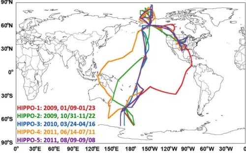
campaigns measured various atmospheric constituents over the Pacific from 2009 to 2011 (Wofsy, 2011) (see Fig. 1 for flight tracks and times). They provide detailed in-formation on the seasonal and vertical structures of CO over the Pacific (Kort et al., 2012), ideal for studying its spatiotemporal variability and for source attribution.

Analyses of global air pollution and transport are facilitated often by global chemical

25

(4)

ACPD

14, 18961–18996, 2014

GEOS-Chem

Y.-Y. Yan et al.

Title Page

Tables Figures

◭ ◮

Back Close

Full Screen / Esc

Discussion

P

a

per

|

Discus

sion

P

a

per

|

Discussion

P

a

per

|

Discussion

P

a

per

|

2008b, 2014; Zhang et al., 2008; Fiore et al., 2009; Liu et al., 2013). Global CTMs nor-mally have a horizontal resolution of 200–500 km (Fiore et al., 2009; Lamarque et al., 2013), not able to capture nonlinear processes at various fine scales over the pollutant source regions. Over the past decades, nested CTMs with much increased horizontal resolutions have been developed by the global CTM community (e.g., GEOS-Chem

5

(Chen et al., 2009) and TM5, Krol et al., 2005) to better study air pollution charac-teristics over major pollutant source regions. For similar purposes, regional air quality models such as AQM, CMAQ and WAF-Chem have also been established with high horizontal resolutions (Huang et al., 2008; Lam and Fu, 2009; Pfister et al., 2011). These regional or nested models often obtain lateral boundary conditions (LBCs) of

10

chemicals from global CTM simulations, and they capture many small-scale processes under-represented by global CTMs. However, the high-resolution simulation results are rarely used for feedback to improve global CTM simulations. Such “one-way” combina-tion of global and regional models does not allow for high-resolucombina-tion regional models to help study the global air pollutant transport.

15

In this paper, we use the GEOS-Chem CTM simulations to analyze the tropospheric CO over the Pacific Ocean measured from the five HIPPO campaigns over 2009– 2011. For this purpose, we develop a two-way coupler, PeKing University CouPLer (PKUCPL), to integrate results of the global GEOS-Chem model (at 2.5◦ _long.

×2◦ lat.) and its three nested models (at 0.667◦ _long.

×0.5◦ lat.). These nested models

20

cover Asia (Chen et al., 2009), North America (Zhang et al., 2011) and Europe (Vinken et al., 2014), respectively. The coupler acquires nested model results to replace global model results within the respective nested domains, in addition to letting the global CTM provide LBCs to the nested models. The coupler minimizes the computational cost of two-way integration by allowing the four models to run parallel to each other.

25

(5)

ACPD

14, 18961–18996, 2014

GEOS-Chem

Y.-Y. Yan et al.

Title Page

Tables Figures

◭ ◮

Back Close

Full Screen / Esc

Discussion

P

a

per

|

Discus

sion

P

a

per

|

Discussion

P

a

per

|

Discussion

P

a

per

|

HIPPO campaigns, evaluating simulation results from the global model and the two-way coupled model. The analysis is focused on the seasonal and vertical variability of CO, with important implications found for using the coarse-resolution global model to constrain CO emissions. Section 5 concludes the present study.

2 GEOS-Chem and the two-way coupling framework

5

2.1 GEOS-Chem models

Both the global and three nested GEOS-Chem CTMs (version 08-03-02; http://wiki.seas.harvard.edu/geos-chem/index.php/Main_Page) are driven by the GEOS-5 assimilated meteorological data from the National Aeronautic and Space Ad-ministration Global Modeling and Assimilation Office. The nested models are run at

10

a horizontal resolution of 0.667◦_long.

×0.5◦lat. native to the GEOS-5 data (see Fig. 2a for nested domains). The global model is run at a reduced resolution of 2.5◦_long.

×2◦ lat. with meteorological data regridded from the high-resolution GEOS-5 data. All mod-els have 47 vertical layers.

All models are run with the full O_x-NO_x-VOC-CO-HO_xgaseous chemistry with online

15

aerosol calculations. Model convection follows a modified Relaxed Arakawa–Schubert scheme (Rienecker et al., 2008). Vertical mixing in the planetary boundary layer is parameterized with a non-local scheme (Holtslag and Boville, 1993; Lin and McElroy, 2010).

Global anthropogenic emissions of nitrogen oxides (NOx), CO and non-methane

20

volatile organic compounds (NMVOC) are taken from the EDGAR 3.2-FT2000 dataset (Olivier et al., 2005). Emissions over Asia, North America and Europe are further re-placed by various regional inventories shown in Table 1. Emission data are available at 1◦ _long.

×1◦ lat. or finer resolutions, and are regridded to model resolutions prior to the simulation of photochemistry. No interannual variability is imposed. Over Asia,

25

(6)

ACPD

14, 18961–18996, 2014

GEOS-Chem

Y.-Y. Yan et al.

Title Page

Tables Figures

◭ ◮

Back Close

Full Screen / Esc

Discussion

P

a

per

|

Discus

sion

P

a

per

|

Discussion

P

a

per

|

Discussion

P

a

per

|

2012). Figure 3a shows that global annual anthropogenic emissions of CO amount to to about 590 Tg yr−1_{with weak seasonality below 20 %.}

Monthly biomass burning emissions are taken from the GFED2 dataset (van der Werf et al., 2006), with CO emissions updated to GFED3.1 (van der Werf et al., 2010). Figure 3b shows that global monthly biomass burning emissions of CO vary between

5

6.3 and 96 Tg month−1_{over the course of 2008–2011, depending on the climatic}

condi-tions. Over the nested domains (Fig. 3b), biomass burning emissions of CO vary more drastically with time.

Other emissions are calculated online, which is dependent of model meteorology and resolution. Lightning emissions of NO_xare parameterized based on cloud heights

10

(Price et al., 1997), with a local adjustment based on the OTD/LIS satellite measure-ments (Sauvage et al., 2007; Murray et al., 2013) and a backward “C-shape” verti-cal profile (Ott et al., 2010). Soil emissions of NOx follow Yienger and Levy (1995)

and Wang et al. (1998). Biogenic emissions of NMVOC follow MEGAN v2.1 (Guenther et al., 2006).

15

For 2009, global emissions from all sources used in the coarse-resolution global model are about 45 Tg N yr−1 _{for NO}

x and 587 Tg C yr− 1

for NMVOC. Due to the resolution-dependent online calculation of biogenic NMVOC emissions and soil and lightning NOxemissions, the global all-source emissions in the two-way coupled model

are larger than those in the global model by 5 % for NMVOC and by 1 % for NO_x.

20

Figure 3c presents illustrative horizontal distributions of emissions over eastern China (part of the Asian nested domain). It shows that the spatial variability of emis-sions are much better resolved on the nested grid than on the global grid. As detailed in Sect. 3.2, better resolved emissions contribute to a significantly improved simulation of CO.

25

Simulations of both the global model and the two-way coupled model are conducted from July 2008 through 2011 to analyze the tropospheric CO during the HIPPO cam-paigns. Initial conditions of chemicals are regridded from a simulation at 5◦ _long.

(7)

ACPD

14, 18961–18996, 2014

GEOS-Chem

Y.-Y. Yan et al.

Title Page

Tables Figures

◭ ◮

Back Close

Full Screen / Esc

Discussion

P

a

per

|

Discus

sion

P

a

per

|

Discussion

P

a

per

|

Discussion

P

a

per

|

spin-up for our focused analysis over 2009–2011. Ancillary test simulations are also performed over shorter periods (from July 2008 to January or to December 2009) to elaborate the physical mechanisms affecting the CO simulation under the two-way cou-pling framework.

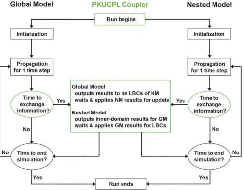
2.2 Two-way coupling setup

5

Figure 4 shows the flowchart to couple the global and nested models. All models are regulated by the PKUCPL coupler. The coupler determines when and how to output global model results to update the LBCs of nested models, and to output nested model results to adjust the global model. Information of all chemical species is exchanged ev-ery three hours between the global and nested models. At the time step for information

10

exchange, the propagation of a particular model is paused until all relevant information has been updated.

Figure 2b illustrates the global and nested model grid cells for information exchange. For a nested model, a buffer zone consisting of three nested grid cells is implemented on each edge of the nested domain (Fig. 2b). At the time to update LBCs, mixing ratios

15

of all chemical species in the buffer zone are taken directly from the respectively grid cells of the global model. A more detailed description of the LBC setups can be found in Chen et al. (2009). While providing the LBCs, global model results in the troposphere are replaced by nested model results within the respective nested domains. Specifi-cally, mass concentrations of all chemical species are outputted from nested models,

20

regridded horizontally to match the global model grid with mass conservation guaran-teed, and then used to replace global model results in the troposphere. Global model grid cells overlapping with the buffer zone of a nested model are not adjusted (Fig. 2b). Under the two-way coupling framework, all models proceed in parallel. The compu-tational time of the coupled system is greater than the slowest individual model (the

25

(8)

ACPD

14, 18961–18996, 2014

GEOS-Chem

Y.-Y. Yan et al.

Title Page

Tables Figures

◭ ◮

Back Close

Full Screen / Esc

Discussion

P

a

per

|

Discus

sion

P

a

per

|

Discussion

P

a

per

|

Discussion

P

a

per

|

OpenMP parallelization for each global or nested model, the coupled system takes about 10 days to finish one simulation year.

2.3 Testing the accuracy of the two-way coupling

Several issues warrant considerations for the two-way coupling. First, the coupled sim-ulation may be affected by the frequency of inter-model data exchange. We find that

5

increasing the exchange frequency from every three hours to every one hour does not affect the CO simulation after the 6 month spin-up period.

In addition, our treatment of LBCs is relatively simplified as the horizontal fluxes of chemicals (Krol et al., 2005) are not accounted for explicitly. This introduces certain random perturbations to the nested models that might in turn affect the global

simula-10

tion in the two-way coupled system. We thus conduct a test two-way coupled simulation that successively increases the LBCs by 5 % for all chemical species at an exchange time step and then decreases the LBCs by 5 % at the next time step. We find that, even with such a large perturbation, the test simulation reproduces the two-way coupled simulation without the 5 % perturbation after the 6 month spin-up period.

15

Furthermore, mass conservation is required in regridding the nested model results to modify the global model. To address the mass conservation issue, we conduct ad-ditional test simulations by turning o_ffall source and sink processes in both the global model and the two-way coupled model. Since the two simulations use the same initial conditions and only simulate the transport processes, mass conservation means that

20

(9)

ACPD

14, 18961–18996, 2014

GEOS-Chem

Y.-Y. Yan et al.

Title Page

Tables Figures

◭ ◮

Back Close

Full Screen / Esc

Discussion

P

a

per

|

Discus

sion

P

a

per

|

Discussion

P

a

per

|

Discussion

P

a

per

|

3 General comparisons of tropospheric CO and hydroxyl radical simulated by

the two-way coupled model vs. the global model

Figure 5 compares the day-to-day variations of tropospheric mean CO mixing ratios from July 2008 through December 2009 simulated by the global model (black lines) vs. the two-way coupled model (red lines). The spin-up period of July–December 2008 is

5

included to elaborate the propagation differentiating the global model simulation from the two-way coupled simulation. In the three nested domains (Fig. 5b–d), the tropo-spheric mean CO simulated by the global model varies from 70 ppb to 115 ppb over the 1.5 years. CO reaches a maximum in the Northern Hemisphere winter-spring with a minimum in summer, reflecting the seasonal variation in CO sources and lifetime

10

(Liang et al., 2004). The two-way coupled model produces more CO than the global model; the difference in 2009 is about 12.9 ppb (13.9 %) averaged over Asia, 8.9 ppb (11.2 %) over North America, and 9.4 ppb (11.7 %) over Europe.

Globally (Fig. 5a), CO mixing ratios in 2009 simulated by the two-way coupled model is about 7.4 ppb (10.4 %) higher than those simulated by the global model alone. The

15

enhancement is more significant in the Northern Hemisphere (13.3 %); this alleviates the negative bias over the Northern Hemisphere typical for coarse-resolution global models (Naik et al., 2013). The enhancement is smaller in the Southern Hemisphere (6.9 %).

Table 2 further shows the CO budget in 2009. The tropospheric CO loss simulated by

20

(10)

ACPD

14, 18961–18996, 2014

GEOS-Chem

Y.-Y. Yan et al.

Title Page

Tables Figures

◭ ◮

Back Close

Full Screen / Esc

Discussion

P

a

per

|

Discus

sion

P

a

per

|

Discussion

P

a

per

|

Discussion

P

a

per

|

3.1 Propagation differentiating the two-way coupled simulation from the global model

To elucidate how the difference between the two-way coupled model and the global model accumulates, we also conduct simulations with one-way nested models (i.e., no feedbacks to the global model; blue lines in Fig. 5b–d). CO concentrations simulated by

5

the one-way nested models differ slightly from global model results on any given day, but the difference varies from one day to another (as evident from the green lines). On average, the one-way nested models produce daily mean CO higher than the global model by 1.24 ppb over Asia and 0.68 ppb over North America and lower by 0.15 ppb over Europe. Here, the nested models adopt LBCs from the global model every three

10

hours with no influences on the global model, thus the CO difference cannot be ac-cumulated effectively throughout time. With the two-way coupling (red lines), however, these regional differences are used to modify the global model every three hours and, with the long lifetime of CO, are accumulated and carried across the globe.

Figure 5d shows that over Europe, the one-way nested model (blue line) results in

15

lower CO than the global model (black line), while the two-way coupled model (red line) produces higher CO than the global model. This is due to elevated transport of CO produced in Asia and North America via the two-way coupling mechanism. Such interaction between high-resolution simulations in multiple regions was unexplored pre-viously and warrant further research.

20

3.2 Factors differentiating the two-way coupled model from the global model

Table 3 identifies various factors differentiating the two-way coupled model from the global model, taking the simulated CO in January 2009 for analysis. In January 2009, the global tropospheric mean CO simulated by the two-way coupled model is larger than that simulated by the global model by 9.6 %. Various test simulations are

con-25

(11)

fac-ACPD

14, 18961–18996, 2014

GEOS-Chem

Y.-Y. Yan et al.

Title Page

Tables Figures

◭ ◮

Back Close

Full Screen / Esc

Discussion

P

a

per

|

Discus

sion

P

a

per

|

Discussion

P

a

per

|

Discussion

P

a

per

|

tors. As shown below, the contributions of these factors are derived in a linear manner as a first-order estimate.

First, the magnitude of emissions differs between the two simulations. As shown in Sect. 2.1, global all-source emissions are larger in the two-way coupled model than in the global model by 5 % for NMVOC and by 1 % for NOx. The additional NMVOC

emis-5

sions increase the tropospheric CO, whereas the extra NOxemissions have a negative

impact on CO (by increasing the OH content). A test simulation with the global model adopts all emissions in the nested domains from the two-way coupled model at ev-ery time step, via a mass-conserved grid-conversion process. The test simulation in-creases the tropospheric CO in January 2009 by 3.5 % compared to the standard global

10

model (Table 3), roughly representing the e_ffect of di_fferences in emission magnitude between the two-way coupled model and the global model. The residual difference of 6.1 % (i.e., 9.6 % minus 3.5 %) represents the combined effect of all factors other than emission magnitude.

Furthermore, the two-way coupled model better captures the small-scale spatial

vari-15

ability of NOx, NMVOC and CO concentrations in the nested domains with a

conse-quence on the photochemical e_fficiency. Such variability in concentration is driven by the variability in emissions (see Fig. 3c for example), since the two-way coupled model use the same initial conditions as the global model. To derive the effect of small-scale emission variability, we conduct a test simulation of the two-way coupled model by

20

adopting all emissions from the global model at every time step. Here, emissions are regridded from 2.5◦_long.

×2◦lat. to 0.667◦long.×0.5◦lat. in the nested domains such that horizontal variability at scales smaller than 2.5◦_long.

×2◦lat. are not resolved. As a result, the test two-way coupled simulation produces higher CO by 1.5 % than the standard global model in January 2009. The 1.5 % difference represents the combined

25

e_ffect of non-emission small-scale variability (related to vertical transport, radiation, and other resolution-dependent processes) that is resolved on the 0.667◦ _long.

×0.5◦ lat. grid but not on the 2.5◦_long.

(12)

ACPD

14, 18961–18996, 2014

GEOS-Chem

Y.-Y. Yan et al.

Title Page

Tables Figures

◭ ◮

Back Close

Full Screen / Esc

Discussion

P

a

per

|

Discus

sion

P

a

per

|

Discussion

P

a

per

|

Discussion

P

a

per

|

minus 1.5 %), contributing about half of the difference between the two-way coupled model and the global model.

3.3 Impacts on tropospheric OH abundance and methyl chloroform lifetime

Table 4 shows the impacts of two-way coupling on the tropospheric OH budget. Con-sistent with the increased CO content, the air mass weighted global mean tropospheric

5

OH in 2009 simulated by the two-way coupled model is lower than that simulated by the global model by 4.2 % (11.9×105vs. 12.4×105molec cm−3). The 4.2 % difference ex-ceeds the standard deviation of OH interannual variation estimated at 2.3 % (Montzka et al., 2011). The OH reduction is more significant in the Northern Hemisphere (5.7 %) than in the Southern Hemisphere (2.1 %), reducing the northern/southern hemispheric

10

OH ratio from 1.27 to 1.24. This change helps alleviate the overestimate in hemispheric OH contrast typical for coarse-resolution global CTMs (Naik et al., 2013). The produc-tion and loss rates of OH are affected insignificantly, however (Table 4). For example, the loss via OH+CO reaction changes marginally due to the increased CO concentra-tion compensating for the decreased OH.

15

The reduced OH abundance leads to an enhanced lifetime of methyl chloroform via tropospheric OH from 5.3 yr to 5.5 yr, a 4.2 % increase. The enhanced lifetime is closer to the observation-based estimate at 6.0–6.3 yr (Prinn et al., 2005; Prather et al., 2012).

4 Evaluation of simulated CO over the Pacific during the five HIPPO campaigns

4.1 Selection of HIPPO CO data and coincident model results

20

Figure 1 shows the flight tracks and dates of five HIPPO aircraft campaigns conducted in various seasons between 2009 and 2011. These campaigns were designed to mea-sure atmospheric trace constituents in the remote troposphere over the Pacific, Arctic, and near-Antarctic regions (Wofsy, 2011). In these campaigns, aircrafts took offin cen-tral North America, flied northward to almost 85◦_{N, turned southward until 75}◦_{S, and}

(13)

ACPD

14, 18961–18996, 2014

GEOS-Chem

Y.-Y. Yan et al.

Title Page

Tables Figures

◭ ◮

Back Close

Full Screen / Esc

Discussion

P

a

per

|

Discus

sion

P

a

per

|

Discussion

P

a

per

|

Discussion

P

a

per

|

finally went back to North America. The measurements provide a large quantity of global-scale high-quality data for analysis of atmospheric chemistry in these remote areas.

During HIPPO, CO was measured by direct absorption spectroscopy using the Har-vard University/Aerodyne Research Quantum Cascade Laser Spectrometer (Jimenez

5

et al., 2005; Kort et al., 2012). To evaluate GEOS-Chem simulations, this study uses the merged dataset providing the tropospheric CO mixing ratios at a vertical resolution of 0.1 km (see http://hippo.ornl.gov/node/16). A total of 620 vertical profiles over the Pa-cific Ocean are employed, with 124 profiles from HIPPO-1, 98 from HIPPO-2, 103 from HIPPO-3, 143 from HIPPO-4, and 152 from HIPPO-5. Model CO are sampled at the

10

times and locations of individual measurements to ensure spatiotemporal consistency with the HIPPO data.

4.2 General spatiotemporal pattern of the Pacific CO during HIPPO

Figure 6a shows the time-height distribution of CO mixing ratios over the Pacific mea-sured from the five campaigns. Most measurements are concentrated below 10 km,

15

especially below 9 km. Below 10 km, CO normally exceed 80 ppb at the beginning and end of each campaign measured over the North Pacific, with values normally lower than 70 ppb in between measured over the South Pacific (Wofsy, 2011). The hemispheric contrast is due mainly to the larger sources of CO in the Northern Hemisphere.

Figure 6a shows that the measured North Pacific CO mixing ratios reach a maximum

20

during HIPPO-3 in March–April 2010. This reflects in part the strong Asian biomass burning emissions in the period (Fig. 3b). Asian influences are also enhanced in spring because of increased midlatitude cyclonic activities supplemented by a relatively long lifetime of CO (Liu et al., 2003; Liang et al., 2004). By comparison, the North Pacific CO mixing ratios are lowest during HIPPO-4 and HIPPO-5 over June-September 2011

25

when the lifetime of CO reaches a minimum (Liang et al., 2004).

(14)

ACPD

14, 18961–18996, 2014

GEOS-Chem

Y.-Y. Yan et al.

Title Page

Tables Figures

◭ ◮

Back Close

Full Screen / Esc

Discussion

P

a

per

|

Discus

sion

P

a

per

|

Discussion

P

a

per

|

Discussion

P

a

per

|

coupled simulation is closer to HIPPO CO than the global model, particularly for the high values over the North Pacific. The global model generally underestimates HIPPO CO with a mean bias by−7.2 ppb (−9.2 %) below 9 km; the bias is much larger over the North Pacific (−10.2 ppb,−13.1 %) than over the South Pacific (−1.6 ppb,−2.1 %). This is consistent with the negative bias in the Northern Hemisphere typical for

coarse-5

resolution global CTMs (Naik et al., 2013).

Figure 7 further evaluates the simulated CO mixing ratios in each vertical layer of 1 km thick (Layer 1 for 0–1 km, Layer 2 for 1–2 km, etc.) during the five HIPPO cam-paigns. Compared to the global model, the two-way coupled simulation reduces the mean normalized bias relative to HIPPO CO in all but the 10th, 11th and 12th layers

10

(between 9 km and 12 km). Note that comparisons at higher altitudes, especially above 10 km, are subject to scarcity in measurements (Fig. 6a). In all layers, the two-way coupled model also slightly improves the correlation with HIPPO CO.

4.3 Vertical profile of the Pacific CO during HIPPO

The thick yellow lines in Fig. 8a–e shows the mean vertical distributions of CO

mea-15

sured from individual HIPPO campaigns. In general, the measured CO mixing ratios are larger in the lower and middle troposphere than in the upper troposphere. The largest vertical contrast occurs during HIPPO-3 in March–April 2010, with CO reach-ing 105 ppb near the surface and at around 5–6 km in contrast to a value of 60 ppb at 12 km. The vertical contrast reflects the strong springtime Asian outflow in the lower

20

and middle troposphere (Liu et al., 2003; Liang et al., 2004). By comparison, the ver-tical contrast is only about 10 ppb during HIPPO-4 in June–July 2011, due to strong convective activities in the Northern Hemisphere summer that mix CO more evenly. During HIPPO-5 in August–September 2011, CO mixing ratios change by 20 ppb at around 9 km due to the stratospheric influences, as shown also in model simulations.

25

(15)

ACPD

14, 18961–18996, 2014

GEOS-Chem

Y.-Y. Yan et al.

Title Page

Tables Figures

◭ ◮

Back Close

Full Screen / Esc

Discussion

P

a

per

|

Discus

sion

P

a

per

|

Discussion

P

a

per

|

Discussion

P

a

per

|

(Fig. 8a). Averaged across the five campaigns (Fig. 8f), the two-way coupled simula-tion is within 3 ppb of HIPPO CO below 9 km with an overestimate by 1–5 ppb above 9 km; the mean bias is 1.1 ppb (1.4 %) for 0–9 km and 2.1 ppb (3.1 %) for 0–13 km. The global model also captures the general vertical structure of HIPPO CO, but with negative biases during all campaigns (Fig. 8a–e, black lines). Averaged across the

5

five campaigns (Fig. 8f), the global model underestimates the HIPPO CO by 1–10 ppb throughout the troposphere; the mean bias reaches−6.2 ppb (−8.3 %) for 0–13 km and −7.2 ppb (−9.2 %) for 0–9 km.

4.4 Implications of model resolution dependence for CO emission constraint

The global model is used often to constrain CO emissions, where the mean model bias

10

relative to measurements is attributed to emission errors (Stavrakou and Müller, 2006; Kopacz et al., 2010; Hooghiemstra et al., 2011). Previous studies have discussed un-certainties in model transport (Liu et al., 2010; Jiang et al., 2013) and the OH field (Kopacz et al., 2010; Hooghiemstra et al., 2011) affecting emission constraints. Here we show that the tropospheric CO simulated by the two-way coupled model are much

15

higher than the global model and are much closer to HIPPO measurements, as a con-sequence of improved representation of resolution-dependent emissions, chemistry, physics, and transport. This has important implications for using the global model to constrain CO emissions.

To elaborate this point, we adjust CO emissions in the global model in an attempt

20

to reproduce the two-way coupled simulation. We find that the global model simula-tion can resemble the two-way coupled simulasimula-tion during HIPPO-1, especially below 4 km, by increasing global CO emissions from all sources by 15 % (Fig. 8a, green line). Emission increases with respect to other campaigns are 25 % for HIPPO-2, 15 % for HIPPO-3, 25 % for HIPPO-4, and 35 % for HIPPO-5 (Fig. 8b–e, green lines). Here all

25

(16)

ACPD

14, 18961–18996, 2014

GEOS-Chem

Y.-Y. Yan et al.

Title Page

Tables Figures

◭ ◮

Back Close

Full Screen / Esc

Discussion

P

a

per

|

Discus

sion

P

a

per

|

Discussion

P

a

per

|

Discussion

P

a

per

|

sources. As shown in Table 2, emissions contribute about 38 % of tropospheric CO in 2009, with the residual 62 % attributed to oxidation of methane and NMVOC. The simu-lation results here imply that, when used for emission constraints, the two-way coupled simulation would suggest much lower CO emissions to match measurements than the coarse-resolution global model.

5

5 Conclusions

We develop a two-way coupler, PKUCPL, to integrate the global GEOS-Chem CTM (at 2.5◦ _long.

×2◦ lat.) and its three high-resolution nested models (at 0.667◦ long.×0.5◦ lat.) covering Asia, North America and Europe, respectively. Under the coupling frame-work, the global model provides LBCs of chemicals for the nested models, while the

10

nested models produce high-resolution results to improve the global model within the respective nested domains. The nested models encompass major anthropogenic pol-lutant source regions and better capture many small-scale nonlinear processes under-represented by the global model; and the two-way coupling allows for such improve-ments to have a global impact.

15

Analysis for 2009 show that the tropospheric CO simulated by the two-way coupled model are much higher than those simulated the global model, with a difference by 10.4 % averaged across the globe. The enhancement reaches 13.3 % in the North-ern Hemisphere, alleviating the northNorth-ern hemispheric underestimate typical for global models (Naik et al., 2013). The increase in CO is accompanied by a 4.2 %

reduc-20

tion in global mean tropospheric mean OH, the magnitude of which is larger than the OH interannual variability estimated at 2.3 % (Montzka et al., 2011). The reduction in OH content results in a 4.2 % enhancement (from 5.3 years to 5.5 years) in the methyl chloroform lifetime via reaction with tropospheric OH, bringing it closer to observation-based estimates at 6.0–6.3 yr (Prinn et al., 2005; Prather et al., 2012).

25

(17)

concentra-ACPD

14, 18961–18996, 2014

GEOS-Chem

Y.-Y. Yan et al.

Title Page

Tables Figures

◭ ◮

Back Close

Full Screen / Esc

Discussion

P

a

per

|

Discus

sion

P

a

per

|

Discussion

P

a

per

|

Discussion

P

a

per

|

tion in January 2009. The two-way coupled simulation results in higher CO by 9.6 % in January 2009. We find that a 4.6 % enhancement is due to improved representation of small-scale spatial variability in NOx, NMVOC and CO resolved on the fine grid but not

on the coarse grid. Another 3.5 % enhancement is due to increased soil and lightning emissions of NOx and especially biogenic emissions of NMVOC that are dependent

5

of model meteorology and resolution. And an additional 1.5 % enhancement is due to improved simulation of vertical transport, radiation, and other resolution-dependent processes.

We use the two-way coupled model and the global model to simulate the tropo-spheric CO mixing ratios over the Pacific during the five HIPPO campaigns in various

10

seasons between 2009 and 2011. Both models capture the general seasonal, horizon-tal and vertical distributions of HIPPO CO. Compared to the global model, the two-way coupled model correlates better with HIPPO CO spatiotemporally. Averaged across the five campaigns, CO simulated by the two-way coupled model is within 3 ppb of HIPPO CO below 9 km with a positive bias by 1–5 ppb above 9 km; the mean bias is 1.1 ppb

15

(1.4 %) for 0–9 km and 2.1 ppb (3.1 %) for 0–13 km. The global model underestimates HIPPO CO by 1–10 ppb throughout the troposphere with a mean bias by −6.2 ppb (−8.3 %); the bias is most apparent over the North Pacific, consistent with the northern hemispheric underestimate typical for global models (Naik et al., 2013).

Our test simulations with the global model suggest that increasing the global CO

20

emissions from all sources by about 15 % would lead to CO mixing ratios comparable to those simulated by the two-way coupled model during HIPPO-1, especially below 4 km; the respective emission increases are 25 % for HIPPO-2, 15 % for HIPPO-3, 25 % for HIPPO-4, and 35 % for HIPPO-5. These results imply an important model dependence on horizontal resolution that is largely unaccounted for in the literature on

25

CO emission constraints.

(18)

ACPD

14, 18961–18996, 2014

GEOS-Chem

Y.-Y. Yan et al.

Title Page

Tables Figures

◭ ◮

Back Close

Full Screen / Esc

Discussion

P

a

per

|

Discus

sion

P

a

per

|

Discussion

P

a

per

|

Discussion

P

a

per

|

coupler, it is straightforward to incorporate additional nested models with the same or different horizontal resolutions. In particular, a much finer nested GEOS-Chem model (at 0.3125◦_long.

×0.25◦ lat.) is currently available for North America and under devel-opment for other regions. As such, it is feasible to develop a low-computational-cost multi-regional multi-layer two-way coupling system to facilitate research on the

interac-5

tions between global, regional and local scales. The coupled system will help address questions such as the impacts of megacities and urbanization on pollutant transport, global environment, and climate change (Parrish and Zhu, 2009).

Acknowledgements. This research is supported by the National Natural Science Foundation of China, grant 41175127, and the 973 program, grant 2014CB441303. We acknowledge the free

10

use of HIPPO CO data from http://hippo.ornl.gov/dataaccess. HIPPO is funded by NSF and NOAA. We thank Yuanhong Zhao and Yan Xia for discussions.

References

Akimoto, H.: Global air quality and pollution, Science, 302, 1716–1719, 2003.

Auvray, M. and Bey, I.: Long-range transport to Europe: seasonal variations and

im-15

plications for the European ozone budget, J. Geophys. Res.-Atmos., 110, D11303, doi:10.1029/2004jd005503, 2005.

Chen, D., Wang, Y., McElroy, M. B., He, K., Yantosca, R. M., and Le Sager, P.: Regional CO pol-lution and export in China simulated by the high-resopol-lution nested-grid GEOS-Chem model, Atmos. Chem. Phys., 9, 3825–3839, doi:10.5194/acp-9-3825-2009, 2009.

20

Cooper, O. R., Parrish, D. D., Stohl, A., Trainer, M., Nedelec, P., Thouret, V., Cammas, J. P., Oltmans, S. J., Johnson, B. J., Tarasick, D., Leblanc, T., McDermid, I. S., Jaffe, D., Gao, R., Stith, J., Ryerson, T., Aikin, K., Campos, T., Weinheimer, A., and Avery, M. A.: Increasing springtime ozone mixing ratios in the free troposphere over western North America, Nature, 463, 344–348, doi:10.1038/nature08708, 2010.

25

(19)

Fol-ACPD

14, 18961–18996, 2014

GEOS-Chem

Y.-Y. Yan et al.

Title Page

Tables Figures

◭ ◮

Back Close

Full Screen / Esc

Discussion

P

a

per

|

Discus

sion

P

a

per

|

Discussion

P

a

per

|

Discussion

P

a

per

|

berth, G., Gauss, M., Gong, S., Hauglustaine, D., Holloway, T., Isaksen, I. S. A., Jacob, D. J., Jonson, J. E., Kaminski, J. W., Keating, T. J., Lupu, A., Marmer, E., Montanaro, V., Park, R. J., Pitari, G., Pringle, K. J., Pyle, J. A., Schroeder, S., Vivanco, M. G., Wind, P., Wojcik, G., Wu, S., and Zuber, A.: Multimodel estimates of intercontinental source-receptor relationships for ozone pollution, J. Geophys. Res.-Atmos., 114, D04301, doi:10.1029/2008jd010816,

5

2009.

Guan, D.-B., Lin, J.-T., Davis, S. J., Pan, D., He, K.-B., Wang, C., Wuebbles, D. J., Streets, D. G., and Zhang, Q.: Response to Lopez et al.: Consumption-based accounting helps mitigate global air pollution, P. Natl. Acad. Sci. USA, doi:10.1073/pnas.1407383111, 2014.

Guenther, A., Karl, T., Harley, P., Wiedinmyer, C., Palmer, P. I., and Geron, C.: Estimates

10

of global terrestrial isoprene emissions using MEGAN (Model of Emissions of Gases and Aerosols from Nature), Atmos. Chem. Phys., 6, 3181–3210, doi:10.5194/acp-6-3181-2006, 2006.

Holtslag, A. A. M. and Boville, B. A.: Local versus nonlocal boundary-layer dif-fusion in a global climate model, J. Climate, 6, 1825–1842,

doi:10.1175/1520-15

0442(1993)006<1825:lvnbld>2.0.co;2, 1993.

Hooghiemstra, P. B., Krol, M. C., Meirink, J. F., Bergamaschi, P., van der Werf, G. R., Nov-elli, P. C., Aben, I., and Röckmann, T.: Optimizing global CO emission estimates using a four-dimensional variational data assimilation system and surface network observations, Atmos. Chem. Phys., 11, 4705–4723, doi:10.5194/acp-11-4705-2011, 2011.

20

HTAP: Hemispheric Transport of Air Pollution 2010 Executive SummaryECE/EB.AIR/2010/10 Corrected, United Nations, 2010.

Huang, H. C., Lin, J. T., Tao, Z. N., Choi, H., Patten, K., Kunkel, K., Xu, M., Zhu, J. H., Liang, X. Z., Williams, A., Caughey, M., Wuebbles, D. J., and Wang, J. L.: Impacts of long-range transport of global pollutants and precursor gases on US air quality under future

cli-25

matic conditions, J. Geophys. Res.-Atmos., 113, D19307, doi:10.1029/2007jd009469, 2008. Jiang, Z., Jones, D., Worden, H. M., Deeter, M. N., Henze, D. K., Worden, J., Bowman, K. W.,

Brenninkmeijer, C., and Schuck, T.: Impact of model errors in convective transport on CO source estimates inferred from MOPITT CO retrievals, J. Geophys. Res.-Atmos., 118, 2073– 2083, 2013.

30

(20)

ab-ACPD

14, 18961–18996, 2014

GEOS-Chem

Y.-Y. Yan et al.

Title Page

Tables Figures

◭ ◮

Back Close

Full Screen / Esc

Discussion

P

a

per

|

Discus

sion

P

a

per

|

Discussion

P

a

per

|

Discussion

P

a

per

|

sorption spectrometer, Proc.SPIE5738, Novel In-Plane Semiconductor Lasers IV, 318–331, doi:10.1117/12.597130, 2005.

Kopacz, M., Jacob, D. J., Fisher, J. A., Logan, J. A., Zhang, L., Megretskaia, I. A., Yan-tosca, R. M., Singh, K., Henze, D. K., Burrows, J. P., Buchwitz, M., Khlystova, I., McMil-lan, W. W., Gille, J. C., Edwards, D. P., Eldering, A., Thouret, V., and Nedelec, P.: Global

es-5

timates of CO sources with high resolution by adjoint inversion of multiple satellite datasets (MOPITT, AIRS, SCIAMACHY, TES), Atmos. Chem. Phys., 10, 855–876, doi:10.5194/acp-10-855-2010, 2010.

Kort, E. A., Wofsy, S. C., Daube, B. C., Diao, M., Elkins, J. W., Gao, R. S., Hintsa, E. J., Hurst, D. F., Jimenez, R., Moore, F. L., Spackman, J. R., and Zondlo, M. A.: Atmospheric

10

observations of Arctic Ocean methane emissions up to 82 degrees north, Nat. Geosci., 5, 318–321, doi:10.1038/ngeo1452, 2012.

Krol, M., Houweling, S., Bregman, B., van den Broek, M., Segers, A., van Velthoven, P., Peters, W., Dentener, F., and Bergamaschi, P.: The two-way nested global chemistry-transport zoom model TM5: algorithm and applications, Atmos. Chem. Phys., 5, 417–432,

15

doi:10.5194/acp-5-417-2005, 2005.

Kuhns, H., Etyemezian, V., Green, M., Hendrickson, K., McGown, M., Barton, K., and Pitch-ford, M.: Vehicle-based road dust emission measurement – Part II: Effect of precipitation, win-tertime road sanding, and street sweepers on inferred PM₁₀emission potentials from paved and unpaved roads, Atmos. Environ., 37, 4573–4582, doi:10.1016/s1352-2310(03)00529-6,

20

2003.

Lam, Y. F. and Fu, J. S.: A novel downscaling technique for the linkage of global and regional air quality modeling, Atmos. Chem. Phys., 9, 9169–9185, doi:10.5194/acp-9-9169-2009, 2009. Lamarque, J.-F., Shindell, D. T., Josse, B., Young, P. J., Cionni, I., Eyring, V., Bergmann, D.,

Cameron-Smith, P., Collins, W. J., Doherty, R., Dalsoren, S., Faluvegi, G., Folberth, G.,

25

Ghan, S. J., Horowitz, L. W., Lee, Y. H., MacKenzie, I. A., Nagashima, T., Naik, V., Plum-mer, D., Righi, M., Rumbold, S. T., Schulz, M., Skeie, R. B., Stevenson, D. S., Strode, S., Sudo, K., Szopa, S., Voulgarakis, A., and Zeng, G.: The Atmospheric Chemistry and Cli-mate Model Intercomparison Project (ACCMIP): overview and description of models, sim-ulations and climate diagnostics, Geosci. Model Dev., 6, 179–206,

doi:10.5194/gmd-6-179-30

2013, 2013.

Liang, Q., Jaegle, L., Jaffe, D. A., Weiss-Penzias, P., Heckman, A., and Snow, J. A.:

(21)

ACPD

14, 18961–18996, 2014

GEOS-Chem

Y.-Y. Yan et al.

Title Page

Tables Figures

◭ ◮

Back Close

Full Screen / Esc

Discussion

P

a

per

|

Discus

sion

P

a

per

|

Discussion

P

a

per

|

Discussion

P

a

per

|

and transport pathways of carbon monoxide, J. Geophys. Res.-Atmos., 109, D23s07, doi:10.1029/2003jd004402, 2004.

Lin, J.-T.: Satellite constraint for emissions of nitrogen oxides from anthropogenic, lightning and soil sources over East China on a high-resolution grid, Atmos. Chem. Phys., 12, 2881–2898, doi:10.5194/acp-12-2881-2012, 2012.

5

Lin, J.-T. and McElroy, M. B.: Impacts of boundary layer mixing on pollutant vertical profiles in the lower troposphere: implications to satellite remote sensing, Atmos. Environ., 44, 1726– 1739, doi:10.1016/j.atmosenv.2010.02.009, 2010.

Lin, J.-T., Wuebbles, D. J., and Liang, X. Z.: Effects of intercontinental transport on surface ozone over the United States: present and future assessment with a global model, Geophys.

10

Res. Lett., 35, L02805, doi:10.1029/2007gl031415, 2008a.

Lin, J.-T., Youn, D., Liang, X., and Wuebbles, D.: Global model simulation of summertime U.S. ozone diurnal cycle and its sensitivity to PBL mixing, spatial resolution, and emissions, At-mos. Environ., 42, 8470–8483, doi:10.1016/j.atmosenv.2008.08.012, 2008b.

Lin, J.-T., Pan, D., Davis, S. J., Zhang, Q., He, K., Wang, C., Streets, D. G., Wuebbles, D. J.,

15

and Guan, D.: China’s international trade and air pollution in the United States, P. Natl. Acad. Sci. USA, 111, 1736–1741, doi:10.1073/pnas.1312860111, 2014.

Liu, H. Y., Jacob, D. J., Bey, I., Yantosca, R. M., Duncan, B. N., and Sachse, G. W.: Transport pathways for Asian pollution outflow over the Pacific: interannual and seasonal variations, J. Geophys. Res.-Atmos., 108, 8786–8800, doi:10.1029/2002jd003102, 2003.

20

Liu, J., Logan, J. A., Murray, L. T., Pumphrey, H. C., Schwartz, M. J., and Megretskaia, I. A.: Transport analysis and source attribution of seasonal and interannual variability of CO in the tropical upper troposphere and lower stratosphere, Atmos. Chem. Phys., 13, 129–146, doi:10.5194/acp-13-129-2013, 2013.

Junhua Liu, Logan, J. A., Jones, D. B. A., Livesey, N. J., Megretskaia, I., Carouge, C., and

Ned-25

elec, P.: Analysis of CO in the tropical troposphere using Aura satellite data and the GEOS-Chem model: insights into transport characteristics of the GEOS meteorological products, Atmos. Chem. Phys., 10, 12207–12232, doi:10.5194/acp-10-12207-2010, 2010.

Montzka, S. A., Krol, M., Dlugokencky, E., Hall, B., Jockel, P., and Lelieveld, J.: Small interannual variability of global atmospheric hydroxyl, Science, 331, 67–69,

30

doi:10.1126/science.1197640, 2011.

(22)

ACPD

14, 18961–18996, 2014

GEOS-Chem

Y.-Y. Yan et al.

Title Page

Tables Figures

◭ ◮

Back Close

Full Screen / Esc

Discussion

P

a

per

|

Discus

sion

P

a

per

|

Discussion

P

a

per

|

Discussion

P

a

per

|

Naik, V., Voulgarakis, A., Fiore, A. M., Horowitz, L. W., Lamarque, J.-F., Lin, M., Prather, M. J., Young, P. J., Bergmann, D., Cameron-Smith, P. J., Cionni, I., Collins, W. J., Dalsøren, S. B., Doherty, R., Eyring, V., Faluvegi, G., Folberth, G. A., Josse, B., Lee, Y. H., MacKenzie, I. A., Nagashima, T., van Noije, T. P. C., Plummer, D. A., Righi, M., Rumbold, S. T., Skeie, R., Shindell, D. T., Stevenson, D. S., Strode, S., Sudo, K., Szopa, S., and Zeng, G.: Preindustrial

5

to present-day changes in tropospheric hydroxyl radical and methane lifetime from the At-mospheric Chemistry and Climate Model Intercomparison Project (ACCMIP), Atmos. Chem. Phys., 13, 5277–5298, doi:10.5194/acp-13-5277-2013, 2013.

Olivier, J. G., Van Aardenne, J. A., Dentener, F. J., Pagliari, V., Ganzeveld, L. N., and Pe-ters, J. A.: Recent trends in global greenhouse gas emissions: regional trends 1970–2000

10

and spatial distributionof key sources in 2000, Environm. Sci., 2, 81–99, 2005.

Ott, L. E., Pickering, K. E., Stenchikov, G. L., Allen, D. J., DeCaria, A. J., Ridley, B., Lin, R.-F., Lang, S., and Tao, W.-K.: Production of lightning NO(x) and its vertical distribution calculated from three-dimensional cloud-scale chemical transport model simulations, J. Geophys. Res.-Atmos., 115, D04301, doi:10.1029/2009jd011880, 2010.

15

Parrish, D. D. and Zhu, T.: Clean air for megacities, Science, 326, 674–675, 2009.

Pfister, G. G., Parrish, D. D., Worden, H., Emmons, L. K., Edwards, D. P., Wiedinmyer, C., Diskin, G. S., Huey, G., Oltmans, S. J., Thouret, V., Weinheimer, A., and Wisthaler, A.: Char-acterizing summertime chemical boundary conditions for airmasses entering the US West Coast, Atmos. Chem. Phys., 11, 1769–1790, doi:10.5194/acp-11-1769-2011, 2011.

20

Prather, M. J., Holmes, C. D., and Hsu, J.: Reactive greenhouse gas scenarios: systematic exploration of uncertainties and the role of atmospheric chemistry, Geophys. Res. Lett., 39, L09803, doi:10.1029/2012GL051440, 2012.

Price, C., Penner, J., and Prather, M.: NO_xfrom lightning. 1. Global distribution based on light-ning physics, J. Geophys. Res.-Atmos., 102, 5929–5941, doi:10.1029/96jd03504, 1997.

25

Prinn, R., Huang, J., Weiss, R., Cunnold, D., Fraser, P., Simmonds, P., McCulloch, A., Harth, C., Reimann, S., and Salameh, P.: Evidence for variability of atmospheric hydroxyl radicals over the past quarter century, Geophys. Res. Lett., 32, L07809, doi:10.1029/2004GL022228, 2005.

Rienecker, E., Ryan, J., Blum, M., Dietz, C., Coletti, L., Marin III, R., and Bissett, W. P.: Mapping

30

(23)

ACPD

14, 18961–18996, 2014

GEOS-Chem

Y.-Y. Yan et al.

Title Page

Tables Figures

◭ ◮

Back Close

Full Screen / Esc

Discussion

P

a

per

|

Discus

sion

P

a

per

|

Discussion

P

a

per

|

Discussion

P

a

per

|

Sauvage, B., Martin, R. V., van Donkelaar, A., Liu, X., Chance, K., Jaeglé, L., Palmer, P. I., Wu, S., and Fu, T.-M.: Remote sensed and in situ constraints on processes affecting tropical tropospheric ozone, Atmos. Chem. Phys., 7, 815–838, doi:10.5194/acp-7-815-2007, 2007. Stavrakou, T. and Müller, J. F.: Grid-based versus big region approach for inverting CO

emis-sions using Measurement of Pollution in the Troposphere (MOPITT) data, J. Geophys.

Res.-5

Atmos. (1984–2012), 111, D15304, doi:10.1029/2005JD006896, 2006.

Streets, D. G.: An inventory of gaseous and primary aerosol emissions in Asia in the year 2000, J. Geophys. Res., 108, 8809, doi:10.1029/2002jd003093, 2003.

van der Werf, G. R., Randerson, J. T., Giglio, L., Collatz, G. J., Kasibhatla, P. S., and Arel-lano Jr., A. F.: Interannual variability in global biomass burning emissions from 1997 to 2004,

10

Atmos. Chem. Phys., 6, 3423–3441, doi:10.5194/acp-6-3423-2006, 2006.

van der Werf, G. R., Randerson, J. T., Giglio, L., Collatz, G. J., Mu, M., Kasibhatla, P. S., Mor-ton, D. C., DeFries, R. S., Jin, Y., and van Leeuwen, T. T.: Global fire emissions and the contribution of deforestation, savanna, forest, agricultural, and peat fires (1997–2009), At-mos. Chem. Phys., 10, 11707–11735, doi:10.5194/acp-10-11707-2010, 2010.

15

Vinken, G. C. M., Boersma, K. F., van Donkelaar, A., and Zhang, L.: Constraints on ship NO_x

emissions in Europe using GEOS-Chem and OMI satellite NO₂observations, Atmos. Chem.

Phys., 14, 1353–1369, doi:10.5194/acp-14-1353-2014, 2014.

Wang, Y., Jacob, D. J., and Logan, J. A.: Global simulation of tropospheric O₃-NO_x

-hydrocarbon chemistry, 1. Model formulation, J. Geophys. Res., 103, 10713–10725,

20

doi:10.1029/98JD00158, 1998.

Wild, O. and Akimoto, H.: Intercontinental transport of ozone and its precursors in a three-dimensional global CTM, J. Geophys. Res.-Atmos., 106, 27729–27744, doi:10.1029/2000jd000123, 2001.

Wofsy, S. C.: HIAPER Pole-to-Pole Observations (HIPPO): fine-grained, global-scale

measure-25

ments of climatically important atmospheric gases and aerosols, Philos. T. R. Soc. A, 369, 2073–2086, doi:10.1098/rsta.2010.0313, 2011.

Wuebbles, D. J., Lei, H., and Lin, J. T.: Intercontinental transport of aerosols and pho-tochemical oxidants from Asia and its consequences, Environ. Pollut., 150, 65–84, doi:10.1016/j.envpol.2007.06.066, 2007.

30

(24)

ACPD

14, 18961–18996, 2014

GEOS-Chem

Y.-Y. Yan et al.

Title Page

Tables Figures

◭ ◮

Back Close

Full Screen / Esc

Discussion

P

a

per

|

Discus

sion

P

a

per

|

Discussion

P

a

per

|

Discussion

P

a

per

|

Yu, H., Remer, L. A., Chin, M., Bian, H., Tan, Q., Yuan, T., and Zhang, Y.: Aerosols from overseas rival domestic emissions over North America, Science, 337, 566–569, doi:10.1126/science.1217576, 2012.

Zhang, L., Jacob, D. J., Boersma, K. F., Jaffe, D. A., Olson, J. R., Bowman, K. W., Worden, J. R., Thompson, A. M., Avery, M. A., Cohen, R. C., Dibb, J. E., Flock, F. M., Fuelberg, H. E.,

5

Huey, L. G., McMillan, W. W., Singh, H. B., and Weinheimer, A. J.: Transpacific transport of ozone pollution and the effect of recent Asian emission increases on air quality in North America: an integrated analysis using satellite, aircraft, ozonesonde, and surface observa-tions, Atmos. Chem. Phys., 8, 6117–6136, doi:10.5194/acp-8-6117-2008, 2008.

Zhang, L., Jacob, D. J., Downey, N. V., Wood, D. A., Blewitt, D., Carouge, C. C., van

Donke-10

laar, A., Jones, D. B. A., Murray, L. T., and Wang, Y.: Improved estimate of the policy-relevant background ozone in the United States using the GEOS-Chem global model with 1/2◦

×2/3◦ horizontal resolution over North America, Atmos. Environ., 45, 6769–6776,

doi:10.1016/j.atmosenv.2011.07.054, 2011.

Zhang, Q., Streets, D. G., Carmichael, G. R., He, K. B., Huo, H., Kannari, A., Klimont, Z.,

15

(25)

ACPD

14, 18961–18996, 2014

GEOS-Chem

Y.-Y. Yan et al.

Title Page

Tables Figures

◭ ◮

Back Close

Full Screen / Esc

Discussion

P

a

per

|

Discus

sion

P

a

per

|

Discussion

P

a

per

|

Discussion

P

a

per

|

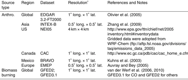
Table 1.Anthropogenic and biomass burning emission inventories used by GEOS-Chem.

Source type

Region Dataset Resolution∗ _{References and Notes}

Anthro. Global EDGAR

3.2-FT2000

1◦_long.

×1◦lat. Olivier et al. (2005)

Asia INTEX-B 0.5◦_long.

×0.5◦lat. Zhang et al. (2009)

US NEI05 4 km×4 km http://www.epa.gov/ttn/chief/net/2005

inventory.html#inventorydata Gridded data were adopted from

WRF-Chem (ftp://aftp.fsl.noaa.gov/divisions/ taq/emissions_data_2005)

Canada CAC 1◦_long.

×1◦lat. http://www.ec.gc.ca/pdb/cac/cac_home_e.cfm

Mexico BRAVO 1◦_long.

×1◦lat. Kuhns et al. (2003)

Europe EMEP 0.5◦_long.

×0.5◦lat. Auvray and Bey (2005)

Biomass burning

Global GFED2;

GFED3.1 1◦

long.×1◦lat. van der Werf et al. (2006, 2010)

GFED3.1 for CO and GFED2 for others

(26)

ACPD

14, 18961–18996, 2014

GEOS-Chem

Y.-Y. Yan et al.

Title Page

Tables Figures

◭ ◮

Back Close

Full Screen / Esc

Discussion

P

a

per

|

Discus

sion

P

a

per

|

Discussion

P

a

per

|

Discussion

P

a

per

|

Table 2.Global budget of tropospheric CO for 2009.

Global model Two-way coupled model

Loss by OH reaction (Tg yr−1₎ ₂₃₆₄ ₂₄₀₀

Transport to stratosphere (Tg yr−1₎ _2.8 _3.3

Production from methane and NMVOC oxidation (Tg yr−1

) 1465 1497

Emissions (Tg yr−1₎ ₉₁₃∗ ₉₁₇∗

Fossil+biofuel 585 589

Biomass burning 328 328

Burden (Tg) 346 383

Tropospheric lifetime (month) 1.75 1.91

∗_{The slight difference of 4 Tg yr}−1

(27)

ACPD

14, 18961–18996, 2014

GEOS-Chem

Y.-Y. Yan et al.

Title Page

Tables Figures

◭ ◮

Back Close

Full Screen / Esc

Discussion

P

a

per

|

Discus

sion

P

a

per

|

Discussion

P

a

per

|

Discussion

P

a

per

|

Table 3.Percentage contributions of individual factors to the difference in January 2009

tropo-spheric CO between the two-way coupled model and the global model, after a 6 month spin-up from July 2008 with consistent initial conditions of chemicals.

Factors % contribution

All factors 9.6 %

A. Emission magnitude (mainly related to biogenic NMVOC) 3.5 %

B. Nonlinear processes within the troposphere 6.1 %

B1. Small-scale horizontal distributions of NO_x, NMVOC, CO, etc. 4.6 %

B2. Other factors 1.5 %

A. Obtained by contrasting simulations of the global model with vs. without adopting the nested model emissions at individual time steps; emissions are regridded from the nested to coarse resolution. B. Residual of “All factors” subtracting A.

B1. Residual of B subtracting B2, as driven by small-scale horizontal distributions of emissions resolved on the nested grid but not on the coarse global grid.

(28)

ACPD

14, 18961–18996, 2014

GEOS-Chem

Y.-Y. Yan et al.

Title Page

Tables Figures

◭ ◮

Back Close

Full Screen / Esc

Discussion

P

a

per

|

Discus

sion

P

a

per

|

Discussion

P

a

per

|

Discussion

P

a

per

|

Table 4.Global budget of tropospheric OH for 2009.

Global model1 Two-way coupled model1

Total loss (Tg yr−1₎ ₃₇₈₀ ₃₇₅₆

OH+CO 1440 (38 %) 1452 (38 %)

OH+CH2₄ 540 (14 %) 516 (14 %)

OH+NMVOC 840 (22 %) 852 (23 %)

OH+O3 204 (5 %) 204 (5 %)

OH+HOy 396 (10 %) 384 (10 %)

OH+NO_y 72 (2 %) 60 (2 %)

OH+H2, SO2, etc. 132 (9 %) 132 (8 %)

Total production (Tg yr−1₎ ₃₇₈₀ ₃₇₅₆

Photolysis of O₃ 1608 (43 %) 1584 (42 %)

Photolysis of other species 480 (12 %) 504 (14 %)

Reactions 1692 (45 %) 1668 (44 %)

Air mass weighted mean concentration (105cm−3₎ _12.4 _11.9

MCF loss rate weighted mean concentration (105cm−3₎ _12.5 _12.1

Methyl chloroform lifetime (yr)3 5.3 5.5

1

In the parentheses is the percentage contribution to total loss or production.

2_{In the simulations, the tropospheric mixing ratio of methane (CH}

4) is fixed at the 2007 level (1732.5 ppb south of 30◦S,

1741.7 ppb between 30◦_{S and Equator, 1801.4 ppb between Equator and 30}◦_{N, and 1855.6 ppb north of 30}◦_N). 3_{Via the reaction with tropospheric OH, defined as 0.92}

·PTi=+1S(∆Pi·A)/ PT

i=1(κi·∆Pi·Ci·A), whereidenotes a layer, T the

(29)

ACPD

14, 18961–18996, 2014

GEOS-Chem

Y.-Y. Yan et al.

Title Page

Tables Figures

◭ ◮

Back Close

Full Screen / Esc

Discussion

P

a

per

|

Discus

sion

P

a

per

|

Discussion

P

a

per

|

Discussion

P

a

per

|

Figure 1.Times and flight tracks of five HIPPO campaigns. Our analysis is focused on CO over

(30)

ACPD

14, 18961–18996, 2014

GEOS-Chem

Y.-Y. Yan et al.

Title Page

Tables Figures

◭ ◮

Back Close

Full Screen / Esc

Discussion

P

a

per

|

Discus

sion

P

a

per

|

Discussion

P

a

per

|

Discussion

P

a

per

|

– –

– – – –

Figure 2. (a)Domains of three nested models covering Asia (70–150◦_{E, 11}◦_S–55◦_{N), North}

(31)

ACPD

14, 18961–18996, 2014

GEOS-Chem

Y.-Y. Yan et al.

Title Page

Tables Figures

◭ ◮

Back Close

Full Screen / Esc

Discussion

P

a

per

|

Discus

sion

P

a

per

|

Discussion

P

a

per

|

Discussion

P

a

per

|

Figure 3. (a) Monthly anthropogenic (fossil+biofuel) emissions of CO within the nested or

global model domains; emissions are unchanged from one year to another. (b) Monthly