www.ann-geophys.net/31/395/2013/ doi:10.5194/angeo-31-395-2013
© Author(s) 2013. CC Attribution 3.0 License.
Annales
Geophysicae
Geoscientiic
Geoscientiic
Geoscientiic
Geoscientiic
Geometry of duskside equatorial current during magnetic storm
main phase as deduced from magnetospheric and low-altitude
observations
S. Dubyagin1, N. Ganushkina1,2, S. Apatenkov3, M. Kubyshkina3, H. Singer4, and M. Liemohn2 1Finnish Meteorological Institute, Erik Palmenin aukio 1, Helsinki, 00101, Finland
2Department of Atmospheric, Oceanic and Space Sciences, University of Michigan, 2455 Hayward St., Ann Arbor, MI 48109-2143, USA
3St. Petersburg State University, Earth Physics Department, Ulyanovskaya 1, Petrodvoretz, St. Petersburg, 198504, Russia 4Space Weather Prediction Center, 325 Broadway, Boulder, CO, USA
Correspondence to:S. Dubyagin ([email protected])
Received: 17 October 2012 – Revised: 16 January 2013 – Accepted: 8 February 2013 – Published: 4 March 2013
Abstract.We present the results of a coordinated study of the moderate magnetic storm on 22 July 2009. The THEMIS and GOES observations of magnetic field in the inner mag-netosphere were complemented by energetic particle obser-vations at low altitude by the six NOAA POES satellites. Ob-servations in the vicinity of geosynchronous orbit revealed a relatively thin (half-thickness of less than 1RE) and intense current sheet in the dusk MLT sector during the main phase of the storm. The total westward current (integrated along the z-direction) on the duskside atr∼6.6REwas comparable to that in the midnight sector. Such a configuration cannot be adequately described by existing magnetic field models with predefined current systems (error inB >60 nT). At the same time, low-altitude isotropic boundaries (IB) of>80 keV pro-tons in the dusk sector were shifted∼4◦ equatorward rela-tive to the IBs in the midnight sector. Both the equatorward IB shift and the current strength on the duskside correlate with the Sym-H∗index. These findings imply a close relation between the current intensification and equatorward IB shift in the dusk sector. The analysis of IB dispersion revealed that high-energy IBs (E >100 keV) always exhibit normal dis-persion (i.e., that for pitch angle scattering on curved field lines). Anomalous dispersion is sometimes observed in the low-energy channels (∼30–100 keV). The maximum occur-rence rate of anomalous dispersion was observed during the main phase of the storm in the dusk sector.
Keywords. Magnetospheric physics (Current systems; En-ergetic particles, precipitating; Storms and substorms)
1 Introduction
The dusk–dawn asymmetry of the magnetic field in the in-ner magnetosphere during storm times has been known for decades (Cahill Jr., 1966). Usually, it is attributed to devel-opment of a partial ring current (PRC) in the dusk–midnight sector (Cummings, 1966; Siscoe and Crooker, 1974; Crooker and Siscoe, 1981; Iijima et al., 1990; Nakabe et al., 1997; Liemohn et al., 2001a). Knowledge of the magnetic configu-ration on the eveningside is very important for space weather applications. Ions, which are the main mass and energy car-riers in the magnetosphere, drift westward after an injec-tion populating the ring current region and eventually influ-ence the outer radiation belts. There is also evidinflu-ence that the PRC can be the main contributor to ground magnetic field disturbances at low latitudes during the storm main phase (Liemohn et al., 2001b). Recent advances in the empirical modeling of the storm time magnetic configuration (Tsyga-nenko and Sitnov, 2007) as well as in the methods of statis-tical analysis (Le et al., 2004) have shown that the duskside current may exhibit significant deviations from the conven-tional shape.
Sergeev et al., 1993). These data have already been used for studying the storm time processes. For example, Hauge and Søraas (1975) noticed that the equatorial boundary of the proton precipitation is well related to the Dst index. In other studies (Søraas et al., 2002; Asikainen et al., 2010), the low-altitude particle observations were used to predict the Dst index. However, there are many factors which make the interpretation of these observations questionable, especially during storm time in the dusk sector. Among them are an uncertainty of the mapping between the equatorial magne-tosphere and low altitudes, and an unknown mechanism of the equatorial isotropic boundary formation. Although there is strong evidence that scattering on curved field lines is the main mechanism of loss cone filling for protons on the night-side (see Sergeev et al., 1993, and references therein), it is not necessarily true during geomagentic storms. It is known that pitch angle scattering by electromagnetic ion cyclotron (EMIC) waves may produce isotropic or almost isotropic proton fluxes at low latitude (Søraas et al., 1980; Gvozde-vsky et al., 1997; Yahnin and Yahnina, 2007, and references therein). Direct spacecraft measurements have shown that EMIC waves are abundant in the inner magnetosphere at dusk during storms (e.g., Br¨aysy et al., 1998; Halford et al., 2010, and references therein).
Given the disparity of conclusions about the location and intensity of current systems in near-Earth space, in this pa-per we investigate this issue with a coordinated data model analysis study. We analyze a moderate storm on 22 July 2009 to determine the geometry of the current system in the dusk sector. The descriptions of the storm and spacecraft orbit con-figuration are given in Sect. 2. In Sect. 3, using THEMIS (Sibeck and Angelopoulos, 2008) and GOES spacecraft ob-servations in the inner magnetosphere, we show that the duskside magnetic configuration in the inner magnetosphere is highly stretched during the storm main phase. In Sect. 4 we use the Tsyganenko and Sitnov (2005) model (hereafter TS05) to figure out whether the standard current systems can reproduce the observed magnetic field. The data of six low-altitude NOAA POES satellites were also available during this storm, providing good MLT and temporal coverage on the storm time-scale. The in situ observations in the equa-torial plane together with TS05 were used to estimate pos-sible mapping inaccuracies. We also attempt to distinguish between the two loss cone filling mechanisms. For that pur-pose, we analyze the dispersion of isotropic boundaries for particles of different energies. These results are presented in Sect. 5. In Sect. 6 we discuss our results in light of previous statistical studies.
2 Event description
The magnetic storm on 22–23 July 2009 was caused by a high-speed stream and has been analyzed in a number of studies (see Ganushkina et al., 2012; Perez et al., 2012, and
22:00 0:00 2:00 4:00 6:00 8:00 10:00 12:00 14:00
July 22 2009, UT
-1000 -500 0 500
AL
AU
-100 -50 0
Sy
m-H
*,
Sy
m-H
-10 0 10
Bz
By
IM
F
0 4 8 12
Pd
yn
(a)
(b)
(c)
(d)
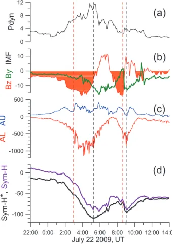
Fig. 1.Solar wind parameters and geomagnetic activity indices: (a)solar wind dynamic pressure in nPa,(b)IMFBz(red) andBy
(green) in nT,(c)AU and AL indices (blue and red curves
respec-tively).(d)Sym-H index (magenta) and Sym-H∗(black). The
ver-tical dashed lines mark the beginning of rapid AL intensifications
(red) and Sym-H∗minima (black).
reference therein). Figure 1 shows solar wind parameters and the geomagnetic activity indices AU, AL, H and Sym-H∗. Sym-H∗is the Sym-H index with the Chapman–Ferraro and ground-induced currents contribution subtracted, Sym-H∗=0.8 Sym-H−13p
Pdyn (e.g., Tsyganenko, 1996). For this storm, Sym-H∗has two minima (−111 nT and−96 nT) at 05:15 and 09:05 UT of 22 July associated with two peri-ods of strong negative IMFBz. The AL index also has two distinct intensifications attaining ∼ −900 and −600 nT at
10 8 6 4 2 0 -2 -4 -6 -8 -10 Y GSM
-8 -6 -4 -2 0 2 4
X GS
M
2 3
4 5
6
3
4 5 6
GOES-11
GOES-12
10 8 6 4 2 0 -2 -4 -6 -8 -10
Y GSM -8
-6 -4 -2 0 2 4
X GSM
8 10
8 10
8 9
8 9
10
GOES-11
GOES-12
THEMIS-D(P3)
THEMIS-E(P4)
(b)
(a)
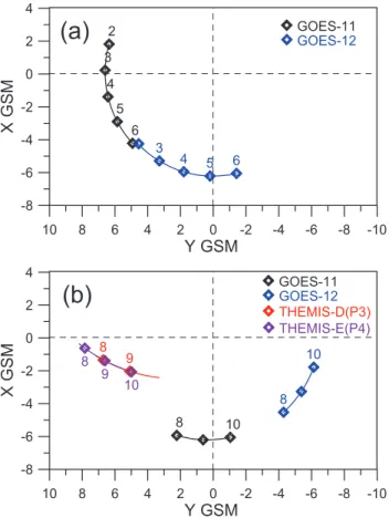
Fig. 2. Projection of spacecraft orbits on the XY GSM plane. (a)The first Sym-H∗dip period (02:00–06:00 UT),(b)second Sym-H∗dip period (08:00–10:00 UT). The colors correspond to different spacecraft.
Fig. 2a) GOES-11 entered the nightside from the dusk sector and GOES-12 moved from∼21:00 MLT to midnight. Dur-ing the second decrease (08:00–09:00 UT, Fig. 2b) THEMIS probes D(P3) and E(P4) successively passed inside geosyn-chronous orbit in the dusk sector∼19:00 MLT when GOES-11 and -12 were at∼23:00 and∼03:00 MLT, respectively.
3 Magnetospheric observations
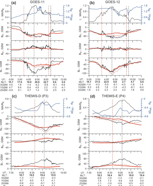
Figure 3 shows observations from four spacecraft in the vicinity of geosynchronous orbit. To represent the magnetic field measurements, we use cylindrical GSM coordinates
(z, r, ϕ)with the z-axis coinciding withzGSM and ther
unit vector is outward from the z-axis andϕis eastward. The three bottom panels in Fig. 3 show thez, ϕ, rcomponents of the external magnetic field (IGRF field has been subtracted). The black curve corresponds to the satellite observations and the red curves correspond to the models that will be discussed later. The blue curves in the top panels show the distance to the neutral sheet (NS) estimated from the Tsyganenko and Fairfield (2004) model. In the near-Earth region, the current
sheet undergoes fewer flapping oscillations and the model es-timation of this parameter is expected to be realistic.
During the first Sym-H∗dip at 02:00–05:15 UT, the mag-netic field at geosynchronous orbit exhibits signatures of an equatorial current enhancement: strengthening of |Br| and decrease ofBz. In the premidnight sector, this enhancement is briefly interrupted by a dipolarization observed by GOES-12 (Fig. 3b) at the beginning of the first AL intensification (marked by a red dashed vertical line). At approximately the same time, the radial component of the external field at GOES-11 (Fig. 3a) in the 18:00–20:00 MLT sector starts to decrease and attains a value of−120 nT. The full field com-ponents (dipole field not subtracted – not shown) observed by GOES-11 at 05:30 UT (the moment of minimumBr) were
Brfull= −153 and Bzfull=17 nT, indicating that the dusk-side magnetic field had an extremely stretched configuration at the geosynchronous location. Using Maxwell’s equation,
µ0j= ∇ ×B, and assuming that∂Bz/∂r << ∂Br/∂z, which is valid for stretched configurations, we can roughly esti-mate the total azimuthal current integrated between +ZSC and−ZSC;I = |Rjϕdz| ≈2|Br(ZSC)|/µ0. HereZSCis the coordinate of the spacecraft position. The black curves in the top panels of Fig. 3 showI=2|Br|/µ0, which is the estimate of total equatorial current per 1REof radial distance. During the first Sym-H∗dip, GOES-11 and -12 were∼0.8RE and ∼1.4REabove the model NS, respectively. As it can be seen in Fig. 3a and b, maximal I values at 20:00 MLT (GOES-11) are higher than at midnight (GOES-12), although GOES-11 is located closer to NS than GOES-12. Since the current sheet in the midnight sector is expected to be thin during the main phase (the TS05 model gives a half-thickness<1RE) and both the duskside and midnight I values are ∼1MA/RE, we conclude that all current on the duskside flows between
−ZSC and +ZSC, implying a current sheet half-thickness ≤1RE.
Similar signatures are seen during the second Sym-H∗dip. The THEMIS probes (Fig. 3c, d) were at∼19:00 MLT and
|dZNS|<0.8RE, closer to the NS than the GOES space-craft were during the first Sym-H∗dip. Again the observa-tions show strengthening of |Br| and decrease of Bz. The full magnetic field components wereBrfull=126 nT,Bzfull=
65 nT (THEMIS D(P3) at r=5.2RE) and Brfull=122 nT,
(a) (b)
(c) (d)
0:00 2:00 4:00 6:00 8:00 10:00 12:00 -120 -80 -40 0 Br , GSM -40 0 40 BM , GS M -80 -40 0 Bz , GSM 0 0.4 0.8 1.2 I, MA/R E 0 0.6 1.2 1.8 dZ NS , R E
15.1 17.0 18.9 20.8 22.7 0.6 2.6
4.5 1.8 -1.4 -4.2 -5.9 -6.1 -4.6 4.7 6.4 6.4 4.9 2.2 -1.0 -4.1 -0.9 0.1 0.7 1.3 1.9 2.5 2.5 UT : MLT : XGSM: YGSM: ZGSM: GOES-11
0:00 2:00 4:00 6:00 8:00 10:00 12:00 -120 -80 -40 0 Br , GSM -40 0 40 BM , GSM -80 -40 0 Bz , GS M 0 0.4 0.8 1.2 I, MA/R E 0 0.6 1.2 1.8 dZ NS
, R
E
GOES-12
19.1 21.0 22.9 0.8 2.7 4.7 6.6
-1.4 -4.3 -5.9 -6.1 -4.5 -1.8 1.4 6.3 4.6 1.8 -1.4 -4.3 -6.1 -6.4 1.6 2.2 2.3 2.3 2.2 1.8 0.6 UT :
MLT : XGSM: YGSM: ZGSM:
7:30 8:00 8:30 9:00 9:30 10:00 0 40 80 120 Br , GSM -40 0 40 BM , GSM -160 -120 -80 -40 Bz , GSM 0 0.4 0.8 I, MA/R E -0.8 -0.4 0 dZ NS , R E UT : MLT : XGSM: YGSM: ZGSM: R:
18.7 19.0 19.4 19.9
-1.3 -1.7 -2.0 -2.3 6.7 6.0 5.1 4.1 -0.6 -0.4 -0.1 0.1 6.9 6.2 5.5 4.7
THEMIS-D (P3)
7:30 8:00 8:30 9:00 9:30 10:00 0 40 80 120 Br , GSM -40 0 40 BM , GSM -160 -120 -80 -40 Bz , GS M 0 0.4 0.8 I, MA/R E -0.8 -0.4 0 dZ NS , R E
18.2 18.4 18.7 19.0 19.4
-0.6 -1.0 -1.4 -1.8 -2.1 7.8 7.3 6.6 5.9 5.0 -1.1 -1.0 -0.8 -0.5 -0.2 7.9 7.4 6.8 6.1 5.4 UT : MLT : XGSM: YGSM: ZGSM: R: THEMIS-E (P4)
Fig. 3. (a)–(d)Observations of four spacecraft. Top panel: the estimate of the total currentI=2Br/µ0in units ofMA/RE(black curve) and
distance to the model neutral sheet (blue curve). The next three panels show theBz,Bϕ, andBrcomponents (dipole field subtracted) in nT:
black – spacecraft observations; red solid curve – TS05 model field; red dashed curve – TS05MOD field. Red and black vertical lines mark beginnings of rapid AL intensifications and Sym-H∗minima, respectively.
total current values estimated at the same radial distance can be compared.
4 Modeling results
It is important to check whether the observed magnetic field signature can be described in terms of classical storm time current systems (PRC, tail current, etc) or if it is a manifesta-tion of some unknown current. We compare the observamanifesta-tions with TS05, a model that comprises all current systems and has been shown to be a good choice for modeling this par-ticular storm (Ganushkina et al., 2012). The red solid curves in Fig. 3 represent the model field components. The largest
deviations of the TS05 field from observations (as large as
∼50–60 nT) are seen inBron the duskside during both Sym-H∗minima periods (Fig. 3a, c). The difference inBzandBϕ
current basically flows outside r=6.6RE and contributes mostly toBzat geosynchronous distance (Ganushkina et al., 2012)). We varied these parameters to minimize the error be-tween the model and spacecraft observations in a manner de-scribed in Ganushkina et al. (2012). The resulting field com-ponents of this modified TS05 model (hereafter TS05MOD) are shown in Fig. 3 by the red dashed lines. From visual in-spection it is clear that this only provides a minor improve-ment of the magnetic field on the duskside in comparison with the TS05 values. TS05MOD can describe the variation inBzbut fails to describe the strongBron the duskside. An inverse problem for a model having three free parameters and matching two/three point vector measurements concentrated at a similar radial distance is likely ill-posed (under-defined). This is why we do not give the resulting parameter values, but rather concentrate on the resulting field. The goal of this modeling is to show that it is impossible to describe the ex-isting configuration with the TS05 current systems without significant changes of their geometry.
5 Low-altitude observations
5.1 Isotropic boundaries
An additional information about the magnetic configura-tion and the processes in the equatorial plane can be ob-tained from low-altitude observations of the isotropic bound-ary (IB). This boundbound-ary separates regions of adiabatic and chaotic regimes of particle motions in the equatorial cur-rent sheet. It also separates regions of particle distribution having empty and filled loss cones and can be determined from low-altitude particle observations. Numerical simula-tions have shown that pitch angle scattering fills the loss cone atRc/ρ≤8 (e.g., Sergeev and Tsyganenko, 1982). HereRc is the minimum field line curvature radius and ρ is maxi-mum particle gyroradius (see Sergeev et al. (1993) and ref-erences therein for more details about IBs). Using this cri-terion, the position of the IB can be determined from mag-netic field models, assuming that there is no other scatter-ing mechanism actscatter-ing in this region. This ratio can be ex-panded asRc/ρ∼Bz2/(∂Br/∂z)≈Bz2/(µ0j ). It shows that the latitude of the IB is highly sensitive to the magnitude of the normal component in the current sheet. The strength of the Bz depression is a rough measure of how much west-ward current flows outside of the observation point. During an equatorial current intensification, a region of strong scat-tering extends toward Earth and IB moves equatorward. For that reason the IB latitude can be used as an indicator of to-tal current strength if there is no other scattering mechanism acting.
Although unambiguous determination of the type of the isotropization mechanism from low-altitude observations is barely possible, valuable information can be obtained from analysis of IBs for particles of different energy. If the IB
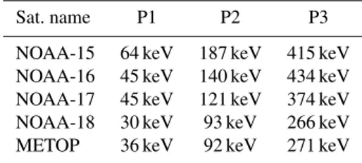
lo-Table 1.Estimated low-energy thresholds for proton 0◦detectors (according to Asikainen et al., 2012).
Sat. name P1 P2 P3
NOAA-15 64 keV 187 keV 415 keV
NOAA-16 45 keV 140 keV 434 keV
NOAA-17 45 keV 121 keV 374 keV
NOAA-18 30 keV 93 keV 266 keV
METOP 36 keV 92 keV 271 keV
cation is controlled byRc/ρ parameter, the IBs of particles having different energy must exhibit dispersion because gy-roradius depends on particle energy. The higher the energy, the lower the latitude of the boundary. The opposite order of IBs is usually interpreted as indication that IBs are formed by wave–particle interactions (e.g., Sergeev et al., 2010). In Sect. 5.3, we analyze the proton energy dispersions to con-clude when and where the usage of Rc/ρ=8 criterion for IB can be justified and we present the comparison of the ob-served and model IBs in Sect. 5.4.
5.2 NOAA/POES particle data
later), this IB cannot be referred to the nominal energy be-cause of the shift of the 0◦-detector low-energy limit. These low-energy limits estimated according to Asikainen et al. (2012) for the year 2009 are given in Table 1. It can be seen that the P1, P2, P3 energy bands always keep their order (P1 – lowest energy; P3 – highest), however, it should be kept in mind that their real energies can be significantly different from the nominal ones, especially for NOAA-15.
An analysis of IB energy dispersion requires a high ac-curacy of determination of IB location because latitudes of IBs of two adjacent energy bands may differ less than 0.1◦. However, uncertainty in calibration factors and other rea-sons (finite temporal resolution, temporal evolution during auroral oval crossings, etc.) only allow the determination of the IB location inside some “confidence interval”. We de-fine the boundaries of this interval as follows (an example is given assuming that the satellite moves from the equator to the pole): the equatorial boundary is the polewardmost point whereF0/F90<0.5 andF0/F90<0.5 for the 4 pre-ceding points (8-s interval); the polar boundary is the first point after the equatorial boundary where F0/F90>0.75 andF0/F90>0.75 for 4 subsequent points. Further in the text, the equatorial and polar latitudes of the IB confidence interval will be referred to as3eqand3pol, respectively. The criterion for3eqwas chosen so that it ignores brief periods of isotropic or nearly isotropic fluxes at the equatorial part of auroral oval which probably are caused by a wave–particle interaction scattering mechanism (Gvozdevsky et al., 1997; Yahnin and Yahnina, 2007). These criteria were used for de-termination of the confidence interval for P1 and P2 IBs. The P3 IB was determined using similar criteria with the weaker condition on the number of points preceding3eqand follow-ing3pol(2 instead of 4). The absolute values of latitudes are used for observations in the Southern Hemisphere in order to combine the observations from both hemispheres.
We applied this algorithm to the auroral oval crossings in both hemispheres in 17:00–24:00, 00:00–07:00 MLT sector in 00:00–12:00 UT interval. After that, we visually inspected all IBs and excluded an insignificant number of incorrect ones. The events with large uncertainty usually correspond to a situation when the regions of isotropic and strongly anisotropic fluxes were separated by a region of transient and weak deviations from isotropy so that the fluxes can-not be considered as purely isotropic or strongly anisotropic. Finally, we have a database of ∼250 proton IB positions for P1, P2, P3 energy bands with information about their uncertainty. On average, the measured counts are one or-der of magnitude lower for each following energy band. For that reason count statistics for P3 band is poorest, with MEPED P3 0◦counts being less than 10 for some of orbits (basically during the prestorm interval). We discarded the IB if the 0◦flux counts were less than 10. It led to a significantly smaller number of P3 IBs detected in comparison with P1 and P2 IBs.
5.3 IB energy dispersion analysis
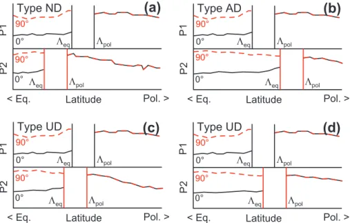
In further analysis we distinguished three IB dispersion types that are illustrated in Fig. 4. This schematic figure shows lat-itude profiles of particle fluxes for 0◦(black curve) and 90◦ (red curve) detectors for P1 and P2 bands. The IB confidence intervals are marked by vertical lines. Figure 4a illustrates the energy dispersion expected for scattering on curved field lines (the P2 IB confidence interval is situated equatorward of that for P1, P13eq>P23pol). This type is referred to as “ND” (normal dispersion). Figure 4b illustrates the oppo-site situation (P23eq>P13pol). We cannot relate this type of dispersion with any certain isotropisation mechanism and we will refer to this type as “AD” (anomalous dispersion). Figure 4c and d illustrate the situation when IB confidence intervals of two energy bands overlap and we can not relate this event with any of the aforementioned types. This dis-persion type is referred to as “UD” (unidentified disdis-persion). These definitions also can be generalized to the usage of three energy bands P1, P2, P3: If every pair of bands has ND dis-persion type, we define this event as ND type. If at least one of the pairs is of AD dispersion type, this event is referred to as AD type. All remaining events are classified as UD type.
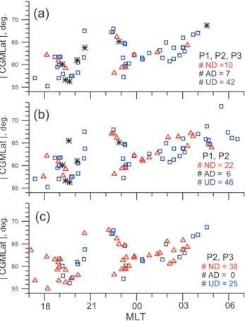
Figure 5a, b, c show locations of observed P2 IB as the cor-rected geomagnetic latitude (CGMLat) vs. MLT for 00:00– 12:00 UT interval. Red, black and blue symbols correspond to ND, AD and UD dispersion types respectively. The differ-ences of the three figures are due to the different combina-tion of energy bands used for classificacombina-tion of the IB disper-sion types. All three energy bands were used for disperdisper-sion classification presented in Fig. 5a, whereas Fig. 5b and c are obtained using P1, P2 and P2, P3 pairs, respectively. There are fewer points in Fig. 5a and c in comparison with Fig. 5b because P3 0◦ flux often does not rise above the 10-count limit and P3 IB cannot be reliably determined. It is obvious that that P3, P2 pair generally exhibits ND dispersion type (no AD type points in Fig. 5c). This important finding may mean that the physical mechanism leading to anomalous dis-persion only affect the particles in the lowest energy range (∼30–80 keV); however, other explanations are also possi-ble. Keeping this fact in mind, we will focus on the anal-ysis of dispersions of the P1 and P2 IBs. Figure 5a and b look similar except for a larger number of points in the latter. Both figures show that AD dispersion types tend to be ob-served in the dusk–midnight MLT sector with only one point in the morning sector. However, one should keep in mind the large number of UD type points in the morning sector. Since most of AD type points in Fig. 5a are also present in Fig. 5b, for the sake of better statistics we further will determine the dispersion type using only the P1, P2 IB pair.
P1
P2
Type ND
Latitude
< Eq. Pol. >
90°
0° /eq /pol
/eq /pol
90°
0°
P1
P2
Type AD
Latitude
< Eq. Pol. >
90°
0° /eq /pol
/eq /pol
90°
0°
P1
P2
Type UD
Latitude
< Eq. Pol. >
90°
0° /eq /pol
/eq /pol
90°
0°
P1
P2
Type UD
Latitude
< Eq. Pol. >
90°
0° /eq /pol
/eq /pol
90°
0°
(a)
(b)
(c)
(d)
Fig. 4.Sketches illustrating criteria for definition of three IB energy dispersion types. P1 and P2 panels correspond to lower and higher energy bands. Vertical lines mark confidence intervals of IB determination (0◦and 90◦fluxes are not shown inside these intervals).
Table 2.Statistics of observation of different types of IB energy dispersion during specific phases of the storm. The phases are defined according to Sym-H∗. IB dispersion type was determined for P1, P2 energy bands.
Phase Interval UT N ND AD UD ND/N AD/N UD/N
prestorm 00:00–02:00 13 6 1 6 46 % 8 % 46 %
main1 02:00–05:20 20 1 3 16 5 % 15 % 80 %
recov1 05:20–08:30 23 6 2 15 26 % 9 % 65 %
main2 08:30–09:10 5 0 0 5 0 % 0 % 100 %
recov2 09:10–12:00 13 9 0 4 69 % 0 % 31 %
and “main2” denote the periods of sharp Sym-H∗decrease. “Recov1” is the period of temporary Sym-H∗ recovery be-tween the two dips and “recov2” is the first part of the main storm recovery period. Columns 4–6 of Table 2 summarize the number of points of the specific dispersion type during the given period and the third column is the total number of points. Columns 7–9 show the percentage of the points of that specific type. Figure 6a graphically presents the data of columns 7–9 of Table 2. It can be seen that the occurrences of ND and UD dispersion types (red and blue bars) behave in the opposite way. The ND occurrence rate is higher during quiet intervals (prestorm and recovery periods) whereas the UD occurrence is higher during both Sym-H∗periods. This behavior can be interpreted as a manifestation of the strength-ening of the radial gradient of the magnetic field in the inner magnetosphere during the main phase so that the P1 and P2 IBs become closer and our algorithm often can not resolve them (the number of UD dispersions increases). The occur-rence of AD type peaks during the first Sym-H∗dip and it is also observed during the prestorm and first Sym-H∗recovery periods. It should be noted that activity in the auroral region
55 60 65 70
| CGM
Lat
|
,
deg.
55 60 65 70
| CGM
Lat
|
,
deg.
MLT
55 60 65 70
| CGMLat |,
deg.
00 21
18 03 06
(a)
(b)
(c)
P1, P2, P3
# ND =10 # AD = 7 # UD = 42
P1, P2
# ND = 22 # AD = 6 # UD = 46
P2, P3
# ND = 38 # AD = 0 # UD = 25
Fig. 5.CGMLat vs. MLT plot of P2 IB positions. Red triangles cor-respond to ND type, black asterisks to AD type and blue squares to UD type. Panels correspond to different dispersion type
classifi-cation methods.(a)involving P1, P2, P3 channels,(b)P1 and P2
channels,(c)P1 and P3 channels, see explanation in the text.
short and only seven IBs were observed during this period. Taking into account that AD occurrence rate never exceeded 14–15 %, this type of dispersion could be easily missed by a satellite during the “dist2” interval. The occurrence rates in Tables 2 and 3 were computed relative to the number of all events when P1 P2 IBs were determined including UD type events. If we compute the AD occurrence rate relative to the number of events when AD or ND dispersion type was iden-tified, 75 % and 56 % rates will be found for “main1” and “dist1” periods, respectively. However, taking into account the limited number of events for analysis and large number of UD type points, these occurrence rates should not be used for comparison with other studies.
5.4 Comparison with the model IBs
The analysis of the measurements in the vicinity of geosta-tionary orbit (Sect. 3) has shown that a relatively thin and intense current sheet exists in the dusk sector and the TS05 model underestimates magnetic field line stretching in this region. On the other hand, the analysis of the IB energy dis-persion (Sect. 5.3) has shown that the anomalous IB
disper-0 50 100
0 500 50 100
O
C
CURRENCE
, %
ND
UD
AD
PRE DIST1 QUIET1 DIST2 QUIET2
(b)
0 50 1000 500 50 100
OCCURRENCE, %
ND
UD
AD
PRE MAIN1 REC1 MAIN2 REC2
(a)
Fig. 6.Occurrence rate of different types of IB dispersions for spe-cific phases of the storm:(a)phases defined according to Sym-H∗, (b)phases defined according to the AL index.
sion type is mostly observed in the dusk and premidnight MLT sectors. However, it was also shown that P2 and P3 IBs never exhibit anomalous dispersion (Fig. 5c). Although it does not necessarily mean that P2 and P3 isotropic bound-aries are formed by scattering on curved field lines in the current sheet region, we compare the observed P2 IBs to the model ones.
Table 3.The same as Table 2 but storm phases are defined according to the AL index.
Phase Interval UT N ND AD UD ND/N AD/N UD/N
prestorm 00:00–02:10 13 6 1 6 46 % 8 % 46 %
dist1 02:10–07:10 35 4 5 26 11 % 14 % 74 %
quiet1 07:10–08:10 7 3 0 4 43 % 0 % 57 %
dist2 08:10–09:30 7 1 0 6 14 % 0 % 86 %
quiet2 09:30–12:00 12 8 0 4 67 % 0 % 33 %
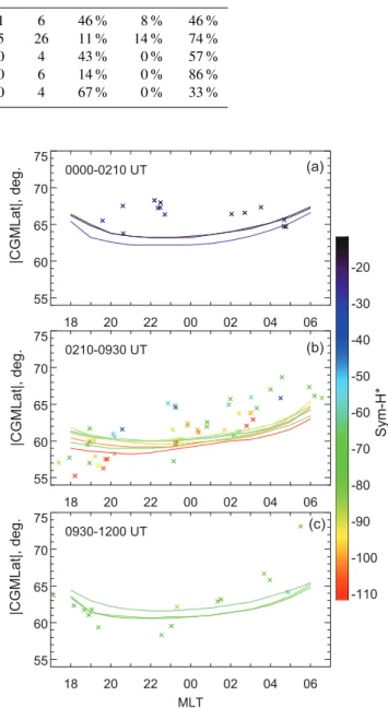
and premidnight sector. It is also the case for the dawnside during the recovery period (Fig. 7c). Note, however, that the points in the dusk sector are in good agreement with TS05 during the recovery phase.
The storm has two intensifications separated by the period of temporary Sym-H∗ recovery (Fig. 1). For simplicity, we do not separate these periods combining all the data during the 02:10–09:30 interval in Fig. 7b. However, the comparison of observed P2 IBs to the model ones in Fig. 7b should be made with precautions. The P2, P3 pair of IBs never shows anomalous dispersion, while the P1, P2 pair sometimes does. At least two hypotheses can be considered: (1) The anoma-lous scattering mechanism only affects the P1 energy range particles, whereas criterionRc/ρ=8 can be used for P2 and P3 IBs. (2) The anomalous scattering mechanism affects the particles in all energy ranges, but the normal dispersion of P2 and P3 IBs is caused by some other reason. Of course, the interpretation of the results presented in Fig. 7 depends on the choice of hypothesis. In general, Fig. 7b demon-strates that the TS05 model underestimates the dusk–dawn asymmetry of the equatorial current during the active phase of the storm because. According to Fig. 5b, there are two ND type points below 58◦CGMLat in the dusk sector and there are no AD type points in the midnight–dawn sector at all. The observed IBs in the duskside sector are on average shifted∼3–5◦ equatorward relative to IBs in the midnight sector. There is a group of IBs in the 17:00–20:00 MLT sec-tor which are 3–4◦ equatorward of the model IB. The two most equatorial IBs (lat.:∼55–56.5◦) were observed during the main Sym-H∗minimum (red color) and were of AD and UD types (see Fig. 5). Three of the most polar IBs around
∼19:00 MLT were observed during the temporary recovery (06:45–08:30 UT).
To check how the PRC intensity influences the IB location, we computed IB positions using TS05 with an increased PRC intensity by a factor×2,×5 and×10. We found that only the factor×5 can produce an IB at∼57◦magnetic latitude on the duskside for this event and a factor×10 produces an IB at∼55◦(the lowest latitude of observed IB).
It should be noted that times of strongestBron the dusk-side (Fig. 3a, c, d) coincide (within 15 min) with times of the two Sym-H∗ minima. To look at this tendency from a dif-ferent angle, we analyze isotropic boundary evolution in the dusk sector. Figure 8 shows the stacked latitudinal profiles
18 20 22 00 02 04 06
55 60 65 70 75
0000-0210 UT
18 20 22 00 02 04 06
55 60 65 70 75
0210-0930 UT
18 20 22 00 02 04 06
MLT 55
60 65 70 75
0930-1200 UT
-20
-30
-40
-50
-60
-70
-80
-90
-100
-110
|CGMLat|, deg.
|CGMLat|, deg.
|CGMLat|, deg.
Sym-H*
(a)
(b)
(c)
Fig. 7.Observed (symbols) and model (curves) isotropic bound-aries during(a)prestorm interval,(b)active phase of the storm and
(c)recovery phase, shown as CGMLat vs. MLT. Color shows
cor-responding Sym-H∗index values.
Fig. 8. Latitudinal profiles of proton number flux (MEPED P2, in log scale) in 17:00–20:00 MLT sector. The panels are plotted
chronologically. The MLT and UT on right and Sym-H∗on the left
correspond to the time the satellite crossed of 60◦CGMLat. Satel-lite name is shown at the vertical axis and the red (black) colors correspond to the auroral oval crossings in the Northern (Southern) Hemispheres. Vertical lines mark IB positions (P1 black; P2 red and P3 blue).
The vertical black, red, and blue lines mark the IB confidence intervals for P1, P2, P3 energy bands, respectively.
-120 -80 -40 0
Sym-H*
54 56 58 60 62 64 66 68 70
| CGMLat |
, deg.
-120 -80 -40 0
Sym-H*
54 56 58 60 62 64 66 68 70
| CGMLat |
,
deg.
MLT: 17-20 R=0.82
MLT: 21-03 R=0.76
(a)
(b)
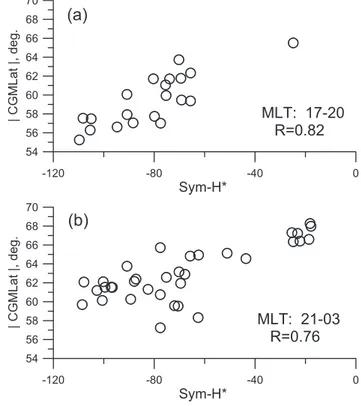
Fig. 9.P2 IB latitude vs. Sym-H∗in the 17:00–20:00 MLT sector(a) and in the 21:00–03:00 MLT sector(b).
A general tendency is that IBs move to the equator when Sym-H∗ decreases, and retreat back to the pole when it re-covers. It is true for all energy bands because the Sym-H∗ -dependent variation of IB positions is much stronger than IBs energy dispersion. It was shown in Sect. 5.3 and it is also seen from Fig. 8 that P3 and P2 IBs (blue and red verti-cal lines) mostly exhibit ND dispersion type. Figure 9 shows P2 IB CGMLat vs. Sym-H∗. Figure 9a corresponds to the IBs in the dusk sector 17:00–20:00 MLT, whereas Fig. 9b shows those determined in the 21:00–03:00 MLT sector. The linear correlation coefficient between the IB latitude and Sym-H∗ were computed. We found a strong correlation in the dusk sector withr=0.82 (N=20) and somewhat weaker corre-lation in the midnight sector (r=0.76, N=34). The corre-lation coefficient between the IB latitude and the AL index were much weaker at 0.56 and 0.13, respectively.
6 Discussion
as close as the geocentric distance∼3–4REduring the peak of the superstorm. So why can it not approach the same dis-tance on the duskside?
However, caution should be used when applyingRc/ρ=8 criterion for interpretation of IB observations during dis-turbed periods. Søraas et al. (2002) interpreted the equato-rial part of the energetic proton precipitation in the evening sector as a freshly injected isotropic plasma. There are many observations supporting a wave-scattering scenario. Mostly, these are magnetospheric and low-altitude observations of the EMIC wave activity in the inner magnetosphere region (Br¨aysy et al., 1998; Erlandson and Ukhorskiy, 2001; Hal-ford et al., 2010). Gvozdevsky et al. (1997) investigated the intense proton precipitation equatorward of the IB which were called LLPP (low-latitude proton precipitation). The examples of such precipitation can be seen in Fig. 8 (last six profiles). The authors found that LLPP particle flux sig-nificantly increases during intense substorms, but also men-tioned that sometimes they could not recognize LLPP during a substorm maximum epoch. They discussed two possible reasons: first, the equatorward motion of IB during disturbed time (the isotopic zone can completely overlap the LLPP re-gion). Second, the increase of the pitch angle diffusion rate so that the fluxes become fully isotropic and the LLPP region cannot be distinguished from isotropic precipitation caused by scattering on the curved field lines. In the latter case, the isotropic boundary is formed by a wave-scattering mecha-nism and the criterionRc/ρ=8 cannot be used.
The MLT distribution of anomalous IB dispersion (Fig. 5b) resembles the distribution of EMIC waves observed by Erlandson and Ukhorskiy (2001). However, the authors found higher occurrence during the recovery phase than dur-ing the main phase. Halford et al. (2010) indeed found that the majority of EMIC waves occur during the main phase but most of the events were observed in the dusk–noon sector and relatively few were observed for MLT>18 h, whereas there were no anomalous IB dispersions observed for MLT<19 h. It is also unclear why higher energy IBs never exhibit anomalous dispersion (Fig. 5c). The decrease of equatorial magnetic field in the inner magnetosphere due to the duskside current strengthening can create favorable con-ditions for EMIC waves generation and ion pitch angle dif-fusion (Kennel and Petschek, 1966). In this case, again, the IB latitude can be considered as an indicator of equatorial current strength.
However, we have presented an analysis of one event and the question arises as to how typical the event might be. Inspection of previous statistical results show that all these findings are inherent features of a magnetic storm.
A manifestation of a strong current on the duskside can be seen in the GOES statistical observations during the main and recovery phases (Ohtani et al., 2007). Comparison of their Fig. 2b and f, showing the disturbance of the radial component of the magnetic field at 03:00–06:00 and 18:00– 21:00 MLT sectors, demonstrates that the dawn–dusk
asym-metry increases with a Sym-H decrease in agreement with our results. The asymmetry is also seen in the depression of
Bz(their Fig. 4a, b).
Statistical comparisons of observedBx, By, BzGSM com-ponents at geosynchronous orbit during storm times and their values predicted by the TS05 model revealed the worst cor-relation forBy(Tsyganenko and Sitnov, 2005). Their scatter plots show that theBy difference can be>100 nT (Tsyga-nenko et al., 2003). However, the y-axis is close to the radial direction if the spacecraft is on the dusk or dawn flanks and strengthening of the duskside current sheet might be respon-sible for this discrepancy.
Our findings are in agreement with results of a storm em-pirical model by Tsyganenko and Sitnov (2007) (by now, the model is available for the list of processed storms, which does not include our studied event). This model does not include predefined current systems, but rather expands the magnetic field into a sum of specific basis functions with co-efficients which are found by fitting to the data. Even though the function defining the current sheet thickness variation over the equatorial plane is defined a priori and is an even function ofY, the model shows that there is a strong current on the duskside during the main phase. Unlike the conven-tional partial ring current, the model current sheet extends from 5 to>10REin radial distance and closes basically on the magnetopause.
The determined latitudes of IBs in the dusk sector during the Sym-H∗minimum period are in agreement with the sta-tistical study of the proton isotropy boundary by Lvova et al. (2005). The authors studied the latitude MLT shape of the IB as a function of solar wind parameters and geomagnetic indices. It was found that the IB can reach∼54–55◦during disturbed times (Dst<−100 nT) in the premidnight sector.
Keeping in mind that the latitude of the IB is a good indica-tor of the equaindica-torial current strength, our results on the MLT dependence of the IB latitude are in agreement with the study of Le et al. (2004), who determined the 3-dimensional cur-rent density by taking the curl of the statistically determined magnetic field. The authors found that the total current (inte-grated from 4 to 8RE inrand−2 to 2REinZ) has a max-imum in the 19:00–21:00 MLT sector for Sym-H<−60 nT. However, the Le et al. (2004) dataset includes both the main and recovery phases, hence the main phase asymmetry can be even stronger.
While none of these previous studies explicitly proves the existence of the thin and strong duskside current sheet, as a group they lend credibility to the concept that such a current could exist, at least temporarily, during the main phase of the storm.
the midnight sector (Fig. 9). It might also mean that the dusk-side current contributes more to Sym-H than the tail current in the midnight sector; however, this suggestion requires a quantitative evaluation.
7 Conclusions
Our analysis of a moderate storm on 22 July 2009 revealed the following:
1. A very strong radial component of the magnetic field was observed in the 18:00–20:00 MLT sector in the vicinity of geosynchronous orbit indicating the develop-ment of a highly stretched configuration with|Br|>> |Bz|during the main phase.
2. A rough estimation of the current sheet half-thickness in the dusk sector gives the value≤1RE.
3. Our tests show that TS05 fails to reproduce the dusk-side magnetic field during this particular storm. More-over, neither a change of azimuthal angle of the PRC maximum nor a variation of its intensity can describe the observed largeBrin the dusk sector.
4. Analyzing the dispersion of proton isotropic boundaries (IBs) we found that IBs of the high-energy pair of chan-nels (E&100 keV) always exhibit normal dispersion (dispersion type expected for pitch angle scattering on curved field lines; IB of the high-energy particles is ob-served at lower latitude than IB of the lower energy particles). However, we found six anomalous IB dis-persion events (of 28 when disdis-persion type identifica-tion could be done) for the two low-energy channels (E.100 keV).
5. All anomalous dispersion events were observed in the dusk–midnight MLT sector and five of them were ob-served during the first AL index intensification. The occurrence of anomalous dispersion is not directly re-lated to storm phase. One event was observed during the prestorm interval and two other events were ob-served during first Sym-H∗recovery period of 06:30– 06:50 UT.
6. Analyzing the∼80 keV proton IB location during the storm peak period we found that the observed IBs in the 17:00–20:00 MLT sector reached∼55◦ magnetic lati-tude. This is∼4◦ equatorward of the model IB. The duskside IBs were on average shifted∼3–5◦ equator-ward relative to IBs in the midnight sector.
7. The latitude of IBs in the 17:00–20:00 MLT sector cor-relates with the Sym-H∗ index with r=0.82 and the correlation is somewhat better than in the midnight sec-tor where it might be influenced by subssec-torms.
8. The difference of 4◦between the observed IBs and the TS05 model IBs in the dusk sector can be achieved by introducing an unrealistic×10 factor to the model PRC intensity.
All of the above findings support a hypothesis that a rela-tively thin (half-thickness <1RE) sheet of current flowing in the azimuthal direction developed on the duskside during the storm main phase. Its sheet-like shape distinguishes this current from the conventional PRC, which has a bean-shaped cross section. We cannot determine how this current closes and whether it is linked to energetic particle injections; how-ever, results of the Tsyganenko and Sitnov (2007) modeling support the hypothesis that its topology is closer to the tail current flowing out through the magnetopause.
Appendix A
Calibration of MEPED 90◦-flux data
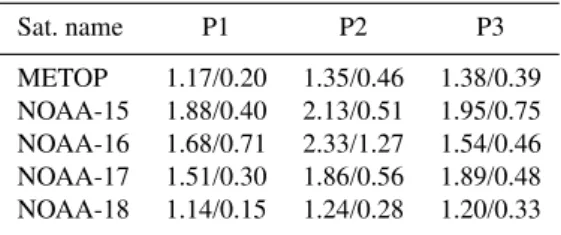
Table A1.(0◦/90◦-flux ratio)/(standard deviation) for P1,P2,P3 pro-ton energy bands.
Sat. name P1 P2 P3
METOP 1.17/0.20 1.35/0.46 1.38/0.39
NOAA-15 1.88/0.40 2.13/0.51 1.95/0.75
NOAA-16 1.68/0.71 2.33/1.27 1.54/0.46
NOAA-17 1.51/0.30 1.86/0.56 1.89/0.48
NOAA-18 1.14/0.15 1.24/0.28 1.20/0.33
Table A2.Linear correlation coefficient/number of data points. The correlation coefficient between 0◦/90◦-flux ratio in the isotropic re-gion and the parameter representing the energy spectrum slope for corresponding energy band (see explanation in the text).
Sat. name P1 P2 P3
METOP −0.31/2097 −0.53/2175 −0.41/921
NOAA-15 −0.69/1147 −0.06/951 −0.58/149
NOAA-16 −0.57/1359 −0.63/1435 −0.32/175
NOAA-17 −0.53/1883 −0.46/1776 −0.36/472
NOAA-18 −0.25/1723 −0.51/1465 −0.30/353
slope for calibration of P3 flux. The correlation coefficients (R, computed for logarithm values) are summarized in Ta-ble A2 with the number of data points.
We performed a linear fit of the logarithm values for all satellites/energy bands except for NOAA-15 P2 (which shows no correlation) and NOAA-16 P3 (there were few data points and the dependence looked strange). For these two we use the median of the calibrating factors from Table A1. To minimize the influence of outliers on the resulting fit, we smoothed the original scattered dependence using the me-dian filter. The 50 data point filtering window size was cho-sen for the P1 and P2 energy bands and 10 data point size for the P3. These smoothed dependences were fitted by a linear equation using an ordinary least-square method. These linear regression coefficients were used to find a calibration factor for every measurement of 90◦flux.
Acknowledgements. The authors thank N. A. Tsyganenko for his help with the TS05 code. Work by SD was supported by an Academy of Finland grant. Magnetospheric indices and solar wind parameters were obtained from the OMNI database provided by J. H. King, N. Papitashvilli at AdnetSystems, NASA GSFC. GOES data were obtained via the CDAWeb. NOAA MEPED particle data have been made publicly available by NOAA. Thanks to K. H. Glassmeier, U. Auster, and W. Baumjohann for the use of FGM data provided under the lead of the Technical University of Braunschweig and with financial support through the German Min-istry for Economy and Technology and the German Center for Avi-ation and Space (DLR) under contract 50 OC 0302. The authors thank the International Space Science Institute in Bern, Switzer-land, for their support of an international team on “Resolving Cur-rent Systems in Geospace”. Work by NG and ML was supported by
NASA and NSF grants.
Topical Editor I. A. Daglis thanks N. A. Tsyganenko and one anonymous referee for their help in evaluating this paper.
References
Asikainen, T., Maliniemi, V., and Mursula, K.: Modeling the contributions of ring, tail, and magnetopause currents to the corrected Dst index, J. Geophys. Res., 115, A12203, doi:10.1029/2010JA015774, 2010.
Asikainen, T., Mursula, K., and Maliniemi, V.: Correction of detector noise and recalibration of NOAA/MEPED en-ergetic proton fluxes, J. Geophys. Res., 117, A09204, doi:10.1029/2012JA017593, 2012.
Br¨aysy, T., Mursula, K., and Marklund, G.: Ion cyclotron waves during a great magnetic storm observed by Freja double-probe electric field instrument, J. Geophys. Res., 103, 4145–4155, doi:10.1029/97JA02820, 1998.
Cahill Jr., L. J.: Inflation of the Inner Magnetosphere dur-ing a Magnetic Storm, J. Geophys. Res., 71, 4505–4519, doi:10.1029/JZ071i019p04505, 1966.
Crooker, N. U. and Siscoe, G. L.: Birkeland Currents as the Cause of the Low-Latitude Asymmetric Disturbance Field, J. Geophys. Res., 86, 11201–11210, doi:10.1029/JA086iA13p11201, 1981. Cummings, W. D.: Asymmetric Ring Currents and the
Low-Latitude Disturbance Daily Variation, J. Geophys. Res., 71, 4495–4503, doi:10.1029/JZ071i019p04495, 1966.
Erlandson, R. E. and Ukhorskiy, A. J.: Observations of electromag-netic ion cyclotron waves during geomagelectromag-netic storms: Wave oc-currence and pitch angle scattering, J. Geophys. Res., 106, 3883– 3895, doi:10.1029/2000JA000083, 2001.
Evans, D. S. and Greer, M. S.: Polar orbiting environmental satellite space environment monitor: 2. Instrument descriptions and archive data documentation, Tech. Memo., OAR SEC-93, NOAA, Boulder, Colorado, 2000.
Ganushkina, N. Y., Dubyagin, S., Kubyshkina, M., Liemohn, M., and Runov, A.: Inner magnetosphere currents during the CIR/HSS storm on July 21–23, 2009, J. Geophys. Res., 117, A00L04, doi:10.1029/2011JA017393, 2012.
Gvozdevsky, B. B., Sergeev, V. A., and Mursula, K.: Long lasting energetic proton precipitation in the inner magneto-sphere after substorms, J. Geophys. Res., 102, 24333–24338, doi:10.1029/97JA02062, 1997.
Halford, A. J., Fraser, B. J., and Morley, S. K.: EMIC wave activity during geomagnetic storm and nonstorm pe-riods: CRRES results, J. Geophys. Res., 115, A12248, doi:10.1029/2010JA015716, 2010.
Hauge, R. and Søraas, F.: Precipitation of>115 keV protons in the evening and forenoon sectors in relation to the magnetic activity, Planet. Space Sci., 23, 1141–1154, 1975.
Iijima, T., Potemra, T. A., and Zanetti, L. J.: Large-Scale Character-istics of Magnetospheric Equatorial Currents, J. Geophys. Res., 95, 991–999, doi:10.1029/JA095iA02p00991, 1990.
Kennel, C. F. and Petschek, H. E.: Limit on stably
trapped particle fluxes, J. Geophys. Res., 71, 1–28,
doi:10.1029/JZ071i001p00001, 1966.
Liemohn, M. W., Kozyra, J. U., Clauer, C. R., and Ridley, A. J.: Computational analysis of the near-Earth magnetospheric current system during two-phase decay storms, J. Geophys. Res., 106, 29531–29542, doi:10.1029/2001JA000045, 2001a.
Liemohn, M. W., Kozyra, J. U., Thomsen, M. F., Roeder, J. L., Lu, G., Borovsky, J. E., and Cayton, T. E.: Dominant role of the asymmetric ring current in producing the stormtime Dst∗, J. Geophys. Res., 106, 10883–10904, doi:10.1029/2000JA000326, 2001b.
Lvova, E. A., Sergeev, V. A., and Bagautdinova, G. R.: Statistical study of the proton isotropy boundary, Ann. Geophys., 23, 1311– 1316, doi:10.5194/angeo-23-1311-2005, 2005.
Nakabe, S., Iyemori, T., Sugiura, M., and Slavin, J. A.: A statistical study of the magnetic field structure in the inner magnetosphere, J. Geophys. Res., 102, 17571–17582, doi:10.1029/97JA01181, 1997.
Ohtani, S., Ebihara, Y., and Singer, H. J.: Storm-time magnetic configurations at geosynchronous orbit: Comparison between the main and recovery phases, J. Geophys. Res., 112, A05202, doi:10.1029/2006JA011959, 2007.
Perez, J. D., Grimes, E. W., Goldstein, J., McComas, D. J., Valek, P., and Billor, N.: Evolution of CIR storm on 22 July 2009, J. Geophys. Res., 117, A09221, doi:10.1029/2012JA017572, 2012. Sergeev, V. A. and Tsyganenko, N.: Energetic particle losses and trapping boundaries as deduced from calculations with a realistic magnetic field model, Planet. Space Sci., 30, 999–007, 1982. Sergeev, V. A., Malkov, M., and Mursula, K.: Testing the Isotropic
Boundary Algorithm Method to Evaluate the Magnetic Field Configuration in the Tail, J. Geophys. Res., 98, 7609–7620, doi:10.1029/92JA02587, 1993.
Sergeev, V. A., Kornilova, T. A., Kornilov, I. A., Angelopoulos, V., Kubyshkina, M. V., Fillingim, M., Nakamura, R., McFadden, J. P., and Larson, D.: Auroral signatures of the plasma injection and dipolarization in the inner magnetosphere, J. Geophys. Res., 115, A02202, doi:10.1029/2009JA014522, 2010.
Sibeck, D. G. and Angelopoulos, V.: THEMIS science ob-jectives and mission phases, Space Sci. Rev., 141, 35–59, doi:10.1007/s11214-008-9393-5, 2008.
Siscoe, G. L. and Crooker, N. U.: On the Partial Ring Cur-rent Contribution to Dst, J. Geophys. Res., 79, 1110–1112, doi:10.1029/JA079i007p01110, 1974.
Soraas, F., Lundblad, J. A., and Hultqvist, B.: On the energy depen-dence of the ring current proton precipitation, Planet. Space Sci., 25, 757–763, 1977.
Søraas, F., Lundblad, J. A., Maltseva, N. F., Troitskaya, V., and Seli-vanov, V.: A comparison between simultaneous I.P.D.P. ground-based observations and observations of energetic protons ob-tained by satellites, Planet. Space Sci., 28, 387–405, 1980. Søraas, F., Aarsnes, K., Oksavik, K., and Evans, D. S.: Ring
cur-rent intensity estimated from low-altitude proton observations, J. Geophys. Res., 107, 1149, doi:10.1029/2001JA000123, 2002. Tsyganenko, N. A.: Effects of the solar wind conditions on the
global magnetospheric configuration as deduced from data-based field models, in: Proceedings of the Third International Confer-ence on Substorms (ICS-3), Versailles, France, 12–17 May 1996, 181–185, 1996.
Tsyganenko, N. A. and Fairfield, D. H.: Global shape of the mag-netotail current sheet as derived from Geotail and Polar data, J. Geophys. Res., 109, A03218, doi:10.1029/2003JA010062, 2004. Tsyganenko, N. A. and Sitnov, M. I.: Modeling the dynamics of the inner magnetosphere during strong geomagnetic storms, J. Geophys. Res., 110, A03208, doi:10.1029/2004JA010798, 2005. Tsyganenko, N. A. and Sitnov, M. I.: Magnetospheric configura-tions from a high-resolution data-based magnetic field model, J. Geophys. Res., 112, A06225, doi:10.1029/2007JA012260, 2007. Tsyganenko, N. A., Singer, H. J., and Kasper, J. C.: Storm-time distortion of the inner magnetosphere: How severe can it get?, J. Geophys. Res., 108, 1209, doi:10.1029/2002JA009808, 2003. Yahnin, A. G. and Yahnina, T. A.: Energetic proton precipitation