The effect of the G1-S transition checkpoint on an age structured cell cycle model.

Structured Cell Cycle Model

Gary S. Chaffey1*, David J. B. Lloyd1, Anne C. Skeldon1, Norman F. Kirkby2

1Department of Mathematics, University of Surrey, Surrey, England,2Department of Chemical Engineering, University of Surrey, Surrey, England

Abstract

Knowledge of how a population of cancerous cells progress through the cell cycle is vital if the population is to be treated effectively, as treatment outcome is dependent on the phase distributions of the population. Estimates on the phase distribution may be obtained experimentally however the errors present in these estimates may effect treatment efficacy and planning. If mathematical models are to be used to make accurate, quantitative predictions concerning treatments, whose efficacy is phase dependent, knowledge of the phase distribution is crucial. In this paper it is shown that two different transition rates at theG1-Scheckpoint provide a good fit to a growth curve obtained experimentally. However, the different transition functions predict a different phase distribution for the population, but both lying within the bounds of experimental error. Since treatment outcome is effected by the phase distribution of the population this difference may be critical in treatment planning. Using an age-structured population balance approach the cell cycle is modelled with particular emphasis on theG1-Scheckpoint. By considering the probability of cells transitioning at theG1-Scheckpoint, different transition functions are obtained. A suitable finite difference scheme for the numerical simulation of the model is derived and shown to be stable. The model is then fitted using the different probability transition functions to experimental data and the effects of the different probability transition functions on the model’s results are discussed.

Citation:Chaffey GS, Lloyd DJB, Skeldon AC, Kirkby NF (2014) The Effect of theG₁- S transition Checkpoint on an Age Structured Cell Cycle Model. PLoS ONE 9(1): e83477. doi:10.1371/journal.pone.0083477

Editor:Raffaele A. Calogero, University of Torino, Italy

ReceivedSeptember 5, 2013;AcceptedNovember 13, 2013;PublishedJanuary 9, 2014

Copyright:ß2014 Chaffey et al. This is an open-access article distributed under the terms of the Creative Commons Attribution License, which permits unrestricted use, distribution, and reproduction in any medium, provided the original author and source are credited.

Funding:GC’s contribution was funded by an Engineering and Physical Sciences Research Council (EPSRC) supported Doctoral Training Centre, funded through EP/P505755/1. There was no other external funding for this project. The funders had no role in study design, data collection and analysis, decision to publish, or preparation of the manuscript.

Competing Interests:The authors have declared that no competing interests exist. * E-mail: g.chaffey@surrey.ac.uk

Introduction

The cell cycle is an ordered set of events that a cell undergoes from its birth until it divides into two daughter cells [1]. In eukaryotic cells the cell cycle may be broken down into four distinct phases, namelyG1,S,G2andM. After birth, a cell enters the longest of the phases, theG1(Gap 1) phase, during which the cell takes on nutrients needed to complete the rest of the cycle. Once the cell has absorbed enough nutrients it may proceed round the cell cycle leaving theG1phase and entering theS(Synthesis) phase. Not all cells leave the G1 phase to enter theS phase, a number of cells enter a quiescent period where they remain viable but leave the cell cycle for a short time, these cells enter the G0 (Gap 0) phase. During theSphase a cell replicates its DNA, at the end of which they have effectively doubled their DNA content. Once DNA synthesis is completed the cell enters theG2(Gap 2) phase. During theG2a cell grows in size and prepares for mitosis. Upon leavingG2the final phaseM(Mitosis) is entered. It is during the mitotic phase that the cell divides, producing two daughter cells. Due to the processes involved in cell division, cells in theM

phase are especially vulnerable to radiotherapy. It should be noted that the M phase may be broken down further into several sub phases, however this is of no consequence for the model discussed herein. The actual length of the cell cycle is variable, this variability mainly occurs in the length of time cells spend in theG1 phase which is governed by the way in which cells ‘transition’ from theG1phase to theSphase [2]. Once a cell commits itself to DNA

synthesis (i.e. enters theS phase) it must continue the cell cycle until division is complete, the ‘transition’ from theG1phase to the Sphase is irreversible.

Chemotherapy drugs can be divided into several types, each of which target a specific process within the cell cycle such as RNA synthesis or cell division. Hence the efficacy of many chemother-apy drugs (e.g. [3], [4] and [5]) is dependent on the cell cycle phase. The radiosensitivity of cells is also phase dependent (e.g. [6], [7] and [8]) with cells in theM (mitotic) phase having their chromosomes arranged in a line prior to separation making them particularly sensitive to ionising radiation. Due to the phase dependent nature of chemotherapy drugs and radiotherapy knowledge of how the cells progress through the different phases is crucial.

There have been a number of mathematical models developed for populations of cells progressing round the cell cycle. Systems of ordinary differential equations may be used to model the growth kinetics of populations of cells however these are too simplistic to capture the intrinsic properties of the cell cycle, but are often an invaluable first step in understanding the kinetics of a population of cells. To adequately model crucial properties of a population of cells such as age, mass or DNA distribution a system of partial differential equations is needed.

property of the cell is used to structure the model, the main properties used being DNA ([12], [13], [14], [15] and [16]), age ([17], [18], [19] and [20]) and mass ([17], [21], [19]).

There are advantages of using a DNA or mass structured model in as much that these quantities may be easily determined experimentally, however such a model contains no information about the age of a particular cell and as such it is possible for cells to remain in the cycle for an infinite amount of time. By use of an age-structured model it is possible to control the length of time a cell may remain in the cell cycle, in particular the G1 phase. Another advantage of age structuring is that, if growth rates and nutrient uptake rates for a given cell line are known, it is possible to determine the mass and DNA content of a cell from its age, however given the cells DNA content or mass it is not possible to determine a cell’s age as there is not a one-to-one mapping between age and DNA or mass.

Analysis has been undertaken to determine the existence and stability of steady size/DNA distributions [22] which may occur under specific circumstances using an age structured model. Population balance models have been used not only on healthy, unperturbed cell lines but also to model the effects of various treatments to cancer cell populations [15], [18], [16] and [23].

In this paper, an age structured cell cycle model is considered together with two different functions governing the movement between the G1 and S phases. Whilst, different functions have been used in the past [18], [20] and [24] little has been done to study the effects of different functions on the phase distributions of cells. It is shown that it is possible to obtain very similar growth curves using different transition functions with the fundamental difference being in the phase distributions for the cells. Although the differences in the phase distributions lie within the range of experimental error for many techniques such as conventional flow cytometry it may be significant in terms of treatment optimisation. The purpose of this paper is to understand how different transition rules may effect the phase distribution of the cells and that whilst the motivation for this analysis is the phase dependent nature of certain treatments these have not been included within the model. This paper is outlined as follows. The age structured model is presented in Section 1 together with a brief overview of the derivation of a generalised transition function in Section 2. Two specific transition functions are then considered. In Section 3 the numerical scheme used for computations is derived. Section 4 sees the age structured model with different transition functions compared with experimental data. The experimental data concerns a batch experiment which was conducted using a mouse-mouse hybridoma cell line (mm321) [25]. The findings of this paper are then summarised together with ideas for future work.

Model Outline

1 Age structured model

The model considered in this paper is divided into three, age-structured sections,G1a,G1bandMAIN as depicted in Figure 1.

The MAIN compartment contains cells in the S, G2 and M phases of the cell cycle, it is at the end of this compartment cell division occurs.

The G1a section contains cells which have just undergone

division. Cells that are in G1a are not able to progress further

round the cell cycle until a fixed time period has elapsed, this represents the minimum age a cell can start replicating its DNA. This is biologically realistic as new cells are normally unable to immediately start replicating their DNA. Once cells have progressed to G1b they undergo transition to the MAIN

compartment at a rate h(v), which is often a function of how long the cell has spent inG1b. It may also be a function of other

factors which effect a cell’s progression round the cell cycle such as nutrient levels, the presence of certain drugs, temperature etc. The

MAINcompartment is of fixed duration and can be thought of as merely a time delay from when a cell leavesG1buntil cell division

and entry of the new daughter cells intoG1a. All compartments

within this model are of a limited duration, theMAIN and G1a

compartments are of a fixed duration and the duration of G1b

varies from zero to some maximum value,TG1b. Biologically, any

cells remaining inG1bat the end ofTG1bwould either die or enter

a quiescent phase. Cells in a quiescent phase may be able to rejoin the cycle at a later time. Neither of these scenarios is modelled here.

In this model the non dimensionalised equations governing the population density of cellsnin each phase are given by

L_nG 1a

L_t z

L_nG 1a

Lt ~0, ð1Þ

L_nG 1b

L_t z

L_nG 1b

Lt zh(v)nG1b~0, ð2Þ

LnMAIN

L_t z

LnMAIN

Lt ~0: ð3Þ

With the corresponding boundary conditions

nG_1a(t,0)~2nMAIN(t,TMAIN),

nG_1b(t,0)~nG_1a(t,TG_1a),

nMAIN(t,0)~

ðTG 1b

0

nG_1a(t,^tt)h(v(^tt))d^tt:

ð4Þ

To complete the model the cell distribution at timet~0needs to be specified, as we are concerned with the system once it has reached exponential growth and steady ‘phase’ distribution this

Figure 1.Overview of a three compartment age structured model.

condition is not important, however for completeness it may be assumed there is a uniform feed of cells into the start of the cell cycle for the firstkhours,

nG_1a(t,0)~c, tvk hours: ð5Þ

This model is of a similar structure to most population balance age-structured models such as those presented in [18] and [20] amongst others. In [20] theMAIN phase is split into three parts

S,G2andM, but since our focus is on the total cell population and the fraction of cells inG1, this difference has no impact. A further difference is in the way that [20] model the transition fromG1, and this will be discussed in greater detail below. In [18], in addition, the G1 phase is modelled as a single compartment rather than divided into two,G1aandG1b.

2 G1-S Transition functions

The probability of a cell leaving theG1bphase and entering the S phase via the transition rule is given by some probability distribution functionf(x)wherexis the variable that determines how likely cells are to undergo transition. Figure 2 gives a graphical representation of such a probability distribution function with phase aget_G

1b acting as the variable controlling the transition

probability. Note that phase age is the length of time a cell spends in a particular phase, For the rest of this paper the subscripts have been removed from the age variable for ease and only used in the case of any ambiguity as to the phase referenced.

Iftvaries by a small amount,dt, then the probability of cells whose age is between t and tzdt transitioning can be approximated by f(t₎dt. Assuming all cells are capable of transitioning given enough nutrients, the total area under the probability distribution curve is one. Therefore the probability that a cell of aget_{has not yet transitioned is given by1}{Ðt

0f(t’)dt’. So the fraction of cells, who have not gone through transition, who go through transition when their age changes fromt_totzdt_is given by

f(t₎dt 1{Ðt

0f(t’)dt’

: ð6Þ

Another way of considering the number of cells going through transition is via a transition rateh(t_{). If the fraction of cells who}

leave in the time period ½t,tzd_t) is given by h(t₎d_t, then by definition this must be equal to equation (6). Therefore, in the limit d_t?0,

h(t₎~ f( t₎

1{Ð₀tf(t’)dt’ dt

dt: ð7Þ

since a cell ages at the same rate as time passest_(t)~t{cwherec

is a constant therefored_dtt~1hence equation (7) simplifies to

h(t)~ f( t₎

1{Ðt 0f(t’)dt’

: ð8Þ

If the cumulative probability of cells transitioning, F(t_{), is} considered then equation (8) may be expressed as

h(t₎~ F’( t₎

1{F(t), ð9Þ

where the dash notation denotes the derivative with respect tot_{. It} is this form of the transition rate which will be used herein.

2.1 Specific transition rules. In this paper, we consider two

different transition functions, the first assumes that the transition rate is constant,h~c, and is therefore independent of the time spent in theG1bphase. Note the transition rateh~ccorresponds

to a cumulative probability of transition given by1{ect

. This is the same form of transition discussed in [18]. This transition rule is not biologically realistic as it implies all cells inG1bhave an equal

probability of progressing to theSphase regardless of how long they have spent acquiring nutrients and preparing for DNA synthesis.

The second form of transition function that we consider is a sigmoidal transition function. This seems biologically reasonable since this implies that the probability of cells progressing to theS

phase immediately after enteringG1b is low due to the limited

amount of nutrients they have absorbed. Once the mass of nutrients absorbed reaches some critical value then the probability of transition is likely to increase considerably, however there will always be a few cells which do not progress to the S phase regardless of nutrient uptake, thus the sigmoidal function attains a maximum value just under one. It should be noted that a sigmoidal cumulative probability function is in keeping with the phase transition seen in cell populations which have been modelled using the kinetics and chemical processes within the cell [26] and [27]. Here we propose a new sigmoidal transition rule governing the probability of transition is proposed, which unlike the one considered in [24] may be non-dimensionalised so there is only one independent parameter, reducing the number of parameters that need to be fitted.

Since a very small proportion of cells ofG1phase age zero it is reasonable to expect that the cumulative distribution function should be non-zero att_G

1b~0. Furthermore, as discussed earlier,

some cells will not transition and enter a quiescent state so the cumulative distribution forG1bremains less than one for alltG1b.

Therefore, the the cumulative distribution function given by

F(t,t₎~₁{ 1 1zeh(Cc

(t,t) Cmax{12)

, ð10Þ

is considered. Here,his related to the maximum and minimum values of the cumulative distribution function andCmaxis related

to the steepness of the sigmoidal function andCc(t,t) represents Figure 2. Probability distribution of transition,f(t)showing the

probability that a cell of agethas not yet transitioned (shaded region) and the probability a cell of agetwill transition in the time intervalttotzdt(dark region).

the amount of glutamine a cell of aget_G

1bhas absorbed at timet.

It then follows that, forhsufficiently large,

h(t,t₎~ h

Cmax L_Cc(t,t)

Lt

eh( Cc(t,t)

Cmax{12)

1zeh(Cc (t,t) Cmax{12)

: ð11Þ

It is reasonable to assume that the rate of change of glutamine is constant, provided there is a high amount of glutamine available.

By making this assumption then LC_Lc(_tt,t)~Rand Cc~tR(It is

assumed that the cell has not taken absorbed any glutamine prior to entering theG1bphase, i.e.Cc~0att~0:). Hence,

h(t₎~ R h

Cmax eh(

tR Cmax{12)

1zeh( tR Cmax{12)

: ð12Þ

The corresponding non-dimensional form of this equation is given by

h(t₎~ e (~tt{h

2)

1z_e(~tt{

h

2)

, ð13Þ

which only has the single parameterhwhich needs to be fitted. In [28] the following expression for the fraction of cells of age t remaining in the G1b phase, n(t,t), for a given intra cellular

glutamine concentrationCG1b(t,tG1b)is proposed

nG1b(t,tG1b) nG1b(t{tG1b,0)

~(CG1b(t,

t_G1b){SMax)2 S2

Max

, ð14Þ

whereSMax is the maximum glutamine content a cell can have

before being forced to go through transition. This leads to the transition function

h(t,t_G1b)~ 2

SMax{CG1b(t,tG1b)

L_CG1b(t,t_G1b)

Lt_G1b : ð15Þ

Note LCG_L1b_t(t,tG1b)

G1b is assumed to always be

§0 so that the

cumulative glutamine never decreases. It can be seen that when

CG1b(t,tG1b)?S_Max, the probability of transition becomes infinite.

Despite this singularity at CG1b(t,tG1b)~SMax this transition

function still provides a very good fit to experimental data [20]. The reasons why this is the case are discussed below.

Numerical Methods

The system of differential equations governing the simplified system described in Section 1 may be solved analytically for specific initial conditions and short time intervals. However, in order to be able to study and manipulate the model for different transition functions for longer time intervals involving many cell cycles it is necessary to use numerical techniques.

3 Derivation of Numerical scheme

In this section a finite difference scheme analogous to the Lax-Wendroff scheme is derived. The Lax-Lax-Wendroff scheme was chosen as it is a second order explicit method and as such yields high accuracy for relatively large time steps where there is a rapid

change or discontinuity such as the initial flow of cells into the main cycle.

For theG1bphase equation (2) may be written as

ntznt~{hn, ð16Þ

Note for ease the time and age dependence has been omitted together with the phase subscript. Subscripts now denote the partial derivatives. Alsohis a function oftonly, furthermore, if the sigmoidal form of the transition rule given in equation (13) is used then

ht~h{h2: ð17Þ

Rearranging and differentiating equation (16) gives

nt~{nt{hn, ð18aÞ

ntt~{ntt{hnt, ð18bÞ

ntt~{ntt{hnt{htn: ð18cÞ

Which, upon using the Taylor expansion together with (17) yields

n(tzd_t,t₎~n 1{d_thz( d_t)2

2 h !

znt{dtz(dt)2h

zntt

(d_t)2 2 zO(dt

3_):

ð19Þ

Finally, standard formulae for the first and second derivatives ofn

with respect totare used, namely

d_n

dt _i,j

~ni,jz1{ni,j{1

2dt , ð20Þ

d2_n

dt2

i,j

~ni,j{1

{2ni,jzni,jz1

(dt₎2 , ð21Þ

whereni,jis the cell density of cells aged½jts,(jz1)ts)in the time

interval ½its,(iz1)ts) where ts and ts are the length of the

discretised elements. This leads to the finite difference scheme

niz1,j~ni,j 1{

(d_t)2 (dt₎2

{d_thi,jz( d_t)2

2 hi,j !

zni,jz1 (d_t)2 2(dt₎2{

d_t

2dtz (d_t)2

2dthi,j !

zni,j{1 (d_t)2 2(dt₎2z

d_t

2dt{ (d_t)2

2dthi,j !

:

ð22Þ

Because of the ‘dispersive’ nature of any numerical difference scheme ifdt=d_{t additional errors are introduced at each time} step. For example if att~₀all cells are age zero and the age step is set toe_{and the time step set to}e

no sense. Similarly if the time step is set to2eafter one step there are no cells present whose age is2esincetƒefor all cells. Hence, additional interpolation is required if the age and time steps are not equal. By settingd_t~dt~aequation(24) becomes

niz1,j~ni,j

a2

2{a

hi,j

zni,jz1 a

2hi,j

zni,j{1 1{ a

2hi,j

:ð23Þ

3.1 Stability of the numerical system. For a numerical

scheme to produce accurate solutions to a partial differential equation, not only must the error at each time step be small enough, any errors must not grow exponentially, i.e. the numerical scheme must also be stable. If the nutrient supply is unlimited and uptake is uniform then the cell cycle may be simplified into two ‘phases’,G1bon it’s own and the remaining phases all put together.

A two compartment model is not suitable for analysing the dynamics of a population of cells as too much information is lost by combining the MAIN phase and G1a phases of the model

discussed in Section 1, in particular the timing of the cell division. However, a two compartment model is sufficient for conducting a stability analysis. Once the system has reached steady growth (i.e. no further input fromG1’) then it may be represented as shown in

Figure 3 whereX andYrepresent the two ‘phases’. To perform the stability analysis the time step matrix is constructed, the norm of which is shown to be bounded. It is helpful to start by defining some notation.

Notation. If the numerical scheme is discretised into elements

of time of lengthtsand age elements of lengthtsthen let cells in

phaseXof age[½it_s,(iz1)t_{s)in the time interval}[½jt_s,(jz1)ts)be

denoted byXi

j. Also let all cells in phase X in the time interval

[½mt_s,(mz_1)tsbe denoted by Xm, where Xm is now a column

vector. Also assume the time line is moved such that at

t~_t0,t’~_{0, where t}’ is the time used for the purposes of the subscript; for convenience the0notation is now dropped.

Construction of time step matrix. Let the maximum

durations of the X and Y phases be Nt_{s and K}t_{s respectively} then at timet~t0,

X0

0 cells enteringX, XN{1

0 cells inxdying due to old age at the next time step, Y0

0 cells enteringY, YK{1

0 cells leavingYand doubling at the next time step: ð24Þ

Clearly,

Xa0~2YK

{1

a{1: ð25Þ

Also the cells enteringYare a function of the cells who were inX

at the previous time step, therefore

Ya0~h(Xa{1), ð26Þ

where h(v) is the probability of transition from X to Y. since nothing happens to the cells during their time inY, it can be thought of as merely a time delay phase, therefore

Yaj~Y j{1

a{1for 1ƒjvK: ð27Þ

Note, the inequality is strictly less thanKas cells of ageKt_shave undergone division and the offspring are now inX0

a.

Assuming a finite central difference scheme is used for calculating the cell densities in theX phase then

X_ai~f(Xi{1 a{1,X

i a{1,X

iz1

a{1) for 1ƒjvN, ð28Þ

and

X_aN~f(XN{1 a{1,X

N

a{1): ð29Þ

From equations (25) and (27) it is clear that

X_a0~2YK{1 a{1~2YK

{2

a{2~. . .~2Ya0{K: ð30Þ Now using equation (26) yields

Xa0~2h(Xa0{K{1): ð31Þ

Equations (25–29) may be expressed in matrix notation as

X0 mz1 X1::N{2

mz1 XN{1

mz1 Y0

mz1 Y1::K{1

mz1 2 6 6 6 6 6 6 4 3 7 7 7 7 7 7 5 ~M X0 m X1::N{2

m XN{1

m Y0

m Y1::K{1

m 2 6 6 6 6 6 6 4 3 7 7 7 7 7 7 5 , ð32Þ

whereMis an(NzK)|(NzK)matrix. To prove the numerical scheme is stable it is sufficient to show [29] that the norm ofMin equation (32) satisfies

M

k kƒ1zka_, ð33Þ

whered_t~dt~aandkis a constant independent ofa. It can be shown that if the trapezium rule is used for approximating equation (26) then the norm ofMis given by

Figure 3. Two Compartment Model. doi:10.1371/journal.pone.0083477.g003

Table 1.Parameters from [20].

Parameter Notation Value

Maximum age inG1aphase TG1a 2.5 hours

Maximum age inG1bphase TG1b 10 hours

Maximum age inSphase TS 5 hours

Maximum age inG2zMphase TG2zM 4 hours

M

k k~supf2,aX

N{2

j~1 h(j)z

a

2(h(0)zh(N{2))g: ð34Þ

For the transition functions considered h is monotonically increasing so

aX

N{2

j~1 h(j)z

a

2(h(0)zh(N{2))ƒa ðXt_max

0

h(t_)dt_{, ð35Þ}

it is therefore sufficient to showaÐXt_max

0 h(t)dtremains bounded. For the sigmoidal transition rule

ðXt_max

0

et{h

2

1ze t{h2

dt~ ln 1ze

t{h

2 h iXtmax

0 , ð36Þ

which for typical h values this is approximately equal to

ln 1zeXt_max{h

2

. ForXt_maxƒh₂then

ln 1zeXt_max{h

2

&1zeXt_max{h

2ƒ2: ð37Þ

ForXt_maxwh₂then

Figure 4. Growth curves produced by using a constant transition rule (a) and a sigmoidal transition rule (b) fitted against experimental batch data presented in[20].

doi:10.1371/journal.pone.0083477.g004

ln 1zeXt_max{h

2

&Xt_max{

h

2: ð38Þ

Thus, in all cases kMk remains bounded. In most cases

Xt_max{h₂

av_{1, this leads to a stronger constraint on the bound}

i.e.kMkƒ2.

Results

In Section 4 it is shown that regardless of whether a constant or a sigmoidal transition rule is used, it is possible to fit the model to a growth curve from experimental data. It is then shown in Section 5 that whilst the different transition functions result in the same growth curve, the fraction of cells in each phase differs.

4 Model validation

Experimental data from [25] was chosen and concerns a batch experiment which was conducted using a mouse-mouse hybrid-oma cell line (mm321). In this experiment 28% of the starting cell

population did not divide but remained viable, 36% of the starting population were evenly distributed in theSphase of the cell cycle and the remaining 36% were initially at the beginning of theG1b

phase. For the purposes of modelling it was assumed the cells starting in theG1bphase were of a phase age between zero and

two hours. The numerical scheme described in Section 3, was implemented using both sigmoidal and constant transition rules. Parameters for the length of different phases were taken from [20], and are stated in Table 1. Theh_{andcparameters were allowed to} vary in the sigmoidal and constant transition rules respectively, until a best fit had been obtained. Several starting values forh_and

cwere used in the optimizations of the fits to ensure the global best fits had been found for each transition rule and that the results were not a local minimum. Optimizations were carried out using Matlab’s [30] least squares curve fitting algorithmlsqcurvefit. The Matlab code for these optimizations is available from [31].

As can be seen in Figure 4, both the constant transition rule (Figure 4a) and the sigmoidal rule (Figure 4b) provide a good fit to the experimental data resulting in residual norm values of 0.1 and 0.2 respectively. The parameters in Table 1 were varied by

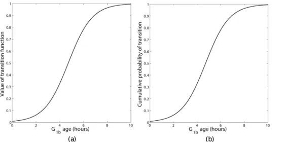
Figure 7. Sigmoidal transition function (a) with the corresponding cumulative probability of transition (b) as a function ofG1bage.

doi:10.1371/journal.pone.0083477.g007

Figure 6. Constant transition function (a) with the corresponding cumulative probability of transition (b) as a function ofG1bage.

+20%. Different values for the Table 1 parameters resulted in different values for the fitted parameters (h_{andc) values but did} not significantly change the goodness of the fit shown in Figure 4 with no residual norms exceeding 0.2. Note that the model did not impose any restrictions on the available nutrients, indicating nutrients were not a limiting factor for cell growth over the course of the experiment. This suggests, that if population growth is the only concern, that a constant transition rule is sufficient.

5 The effect of the transition function

Although the effect of the different transition rules is not apparent in the fitting to the experimental growth curve, here we show that the transition rule does impact on the phase distribution of cells.

In the experimental data used to fit the model the initial population of cells was partially synchronised using a thymidine double block. This partial synchronisation meant the initial population of cells was situated in the S phase and the latter part of theG1phase,G1b. It therefore seems reasonable to assume

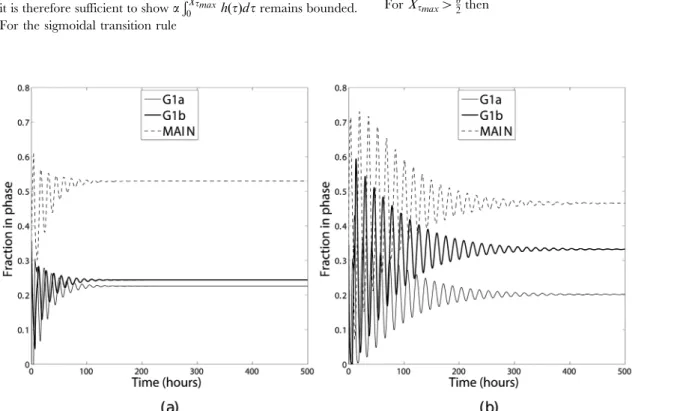
most cells will initially progress round the cycle in a group this would result in the phase distribution being oscillatory. The oscillations would be expected to decay slowly as the synchronicity of the cell population was lost. Such oscillations may be one cause for apparent ‘errors’ in phase distributions obtained from such experiments as the timing of observations would need to occur at known positions on the oscillation, the period of which may not be known. To fully appreciate the differences these transition functions have on the underlying model properties the percentages of cells in each compartment may be compared once transient oscillations have decayed and the system has reached a steady state of phase distributions. The time scale required for the transient oscillations to have decayed sufficiently is of the order of 500 hours and as such it is not feasible to obtain experimental data.

In order to investigate this, the mathematical model was numerically integrated using the same parameters and initial conditions used in Section 4 for long enough that a steady phase distribution had been obtained. The results are shown in Figure 5. These two sets of results differ in two key ways. Firstly, both simulations initially show an oscillation in the phase distribution, however the rate of decay of the oscillations depends on the transition function chosen, with the oscillations decaying much more slowly for a sigmoidal transition function. The difference in the decay rates may be appreciated by considering the area under the cumulative probability function for the different transition functions (Figures 6 and 7). For a steep sigmoidal probability distribution function the area under the curve initially increases slowly then has a rapid increase for a short time interval then returns to a slow increase as shown in Figure 7. This rapid increase would result in the majority of the population remaining in a group as it progressed round the cycle, with each complete cycle dispersing slightly due to the ages corresponding to a low probability of transition. With the value of the constant transition function used in this simulation the area under the corresponding cumulative probability distribution function does not change as rapidly as with the sigmoidal function as shown in Figure 6. This results in the population of cells transitioning more evenly, leading to a more rapid de-synchronisation. Secondly, once the transient oscillations have decayed the percentages of cells in each of the

model’s ‘phases’ differ: in the sigmoidal transition rule there are 20.2%, 33.3% and 46.5% in the G1a, G1b and MAIN phases

respectively, whereas in the constant transition rule these change to 22.6%, 24.4% and 53.0%.

Discussion

In this paper an age-structured cell cycle model has been considered with particular emphasis on theG1-S checkpoint. By considering the probability of cells transitioning at the G1-S checkpoint, different transition functions have been obtained. A suitable numerical scheme for the resulting PDEs has been derived and shown to be numerically stable. This numerical scheme has then been used to look at the effects of the different transition functions on the phase distribution of the cell population.

The model shows there is a noticeable change in the proportion of cells in each phase for the two different transition functions considered. The sigmoidal transition function predicts 53.5% of the cell population being in the G1 phase, whilst the constant transition function places 47.0% of cells in theG1phase.

As mentioned previously the efficacy of chemotherapy treat-ments and the radiosensitivity of cells varies according to a cell’s position in the cell cycle. Since the relationship between cell phase and efficacy may be non-linear a small difference in phase distribution may produce a large change in the efficacy of treatments resulting in the model producing results outside the bounds of experimental error. Therefore, the difference in the phase distributions produced by this model, using the different transition functions, will effect the model’s ability to accurately represent the effects of a given treatment on a population of cells. Consequently, it is important to ascertain the correct transition function if such models are to be used to give a quantitative prediction of the cell population’s response to treatments.

Improvements in techniques may reduce the level of potential error in phase distributions obtained experimentally, this may allow some transition functions to be discounted.

It may also be possible to rigorously derive the form of the transition function for a population of cells by considering the chemical kinetics of a single cell [26].

Whilst there is no consensus on the error on cell phase distributions obtained using flow cytometry [32] the difference in phase distributions produced by the model with the different transition rules lie within the typical bounds of current experi-mental error ([33], [34] and [32]). As noted in Section 5 the difficulty of measuring the phase distribution may be compounded by underlying oscillations induced by the blocking. Thus, the form of the probability distribution function controlling the G1{S checkpoint in an age structured population balance model has little impact on the models ability to fit to experimental data. The lack of effect of the form of the probability transition function explains why the quadratic transition function used in [20] fitted experimental data despite having a singularity. As such a simplified transition function may be used to gain a qualitative understanding of the dynamics of a population of cells.

Author Contributions

Conceived and designed the experiments: GSC DJBL ACS NFK. Analyzed the data: GSC DJBL ACS. Contributed reagents/materials/ analysis tools: GSC DJBL ACS. Wrote the paper: GSC DJBL ACS.

References

1. Alberts B, Bray D, Lewis J, Raff M, Roberts K, et al. (1994) Molecular Biology of the Cell, 3rd Edition. Garland Publishing, New York.

2. Smith J, Martin L (1973) Do cells cycle? Proc Nat Acad Sci USA 70: 1263–1267.

4. Lopes NM, Adams EG, Pitts TW, Bhuyan BK (1993) Cell kill kinetics and cell cycle effects of taxol on human and hamster ovarian cell lines. Cancer chemotherapy and pharmacology 32: 235–242.

5. Owa T, Yoshino H, Yoshimatsu K, Nagasu T (2001) Cell cycle regulation in the g1 phase: a promising target for the development of new chemotherapeutic anticancer agents. Current medicinal chemistry 8: 1487–1503.

6. Brugarolas J, Chandrasekaranl C, Gordoni J, Beachil D, Jacks T (1995) Radiation-induced cell cycle. Nature 377: 12.

7. Marples B,Wouters B, Collis S, Chalmers A, Joiner M(2004) Low-dose hyper-radiosensitivity: a consequence of ineffective cell cycle arrest of radiation-damaged g2-phase cells. Radiation research 161: 247–255.

8. Yao K, Komata T, Kondo Y, Kanzawa T, Kondo S, et al. (2003) Molecular response of human glioblastoma multiforme cells to ionizing radiation: cell cycle arrest, modulation of cyclin-dependent kinase inhibitors, and autophagy. Journal of neurosurgery 98: 378–384.

9. Eakman J, Fredrickson AG, Tsuchiya H (1966) Statistics and dynamics of microbial cell populations. Chemical Engineering Progess, Symposium Series 69: 37–49.

10. Fredrickson AG, Tsuchiya H (1963) Continuous propogation of micro organisms. AIChE Journal 9: 359–468.

11. Fredrickson AG, Ramkrishna D, Tsuchiya H (1967) Statistics and dynamics of correct pro- caryotic cell populations. Mathematical Biosciences 1: 327–374. 12. Liu YH, Bi JX, Zeng AP, Yuan JQ (2007) A population balance model

describing the cell cycle dynamics of myeloma cell cultivation. Biotechnology Progress 23: 1198–1209.

13. Basse B, Baguley BC, Marshall ES, van Brunt WRJB, Wake G, et al. (2003) A mathematical model for analysis of the cell cycle in cell lines derived from human tumors. Journal of Mathematical Biology 47: 295–312.

14. Basse B, Baguley BC, Marshall ES, Wake G, Wall DJN (2005) Modelling the flow of cy-tometric data obtained from unperturbed human tumour cell lines: parameter fitting and comparison. Bulletin of Mathematical Biology 67: 815– 830.

15. Jackiewicz Z, Zubik-Kowal B, Basse B (2009) Finite-difference and pseudo-spectral methods for the numerical simulations of in vitro human tumor cell population kinetics. Mathematical Biosciences and Engineering 6: 561–572. 16. Basse B, Baguley BC, Marshall ES, van Brunt WRJB, Wake G, et al. (2004)

Modelling cell death in human tumour cell lines exposed to the anticancer drug paclitaxel. Journal of Mathematical Biology 49: 329–357.

17. Liou JJ, Srienc F, Fredrickson AG (1997) Solutions of a population balance models based on a successive generations approach. Chemical Engineering Science 52: 1529–1540.

18. Basse B, Ubezio P (2007) A generalised age-and phase-structured model of human tumour cell populations both unperturbed and exposed to a range of cancer therapies. Bulletin of Mathematical Biology 69: 1673–1690.

19. Chapman SJ, Plank M, James A, Basse B (2007) A nonlinear model of age and size-structured populations with applications to cell cycles. The ANZIAM Journal 49: 151–169.

20. Faraday DBF, Hayter F, Kirkby NF (2001) A mathematical model of the cell cycle of a hybridoma cell line. Biochemical Engineering Journal 7: 49–68. 21. Mantzaris NV, Liou JJ, Daoutidis P, Srienc F (1999) Numerical solution of a

mass structured cell population balance model in an environment of changing substrate concentration. Journal of Biotechnology 71: 157–174.

22. Begg RE, Wall DJN, Wake GC (2008) The steady-staes of a multi-compartment, age-size distribution model of cell-growth. European Journal of Applied Mathematics 19: 435–458.

23. Billy F, Clairambault J, Fercoq O (2013) Optimisation of cancer drug treatments using cell population dynamics. Mathematical Methods and Models in Biomedicine.

24. Slater G (2004) Mathematical Modelling of Periodic Feeding in Continuous Cultures of Schiz-zosaccharomyces pombe. Ph.D. thesis.

25. Hayter P (1989) An investigation into the factors that af-fect monoclonal antibody production by hybridomas in culture. http://ethos.bl.uk/OrderDetails. do?did = 14&uin = uk.bl.ethos.329033.

26. Novak B, Tyson JJ (2004) A model for restriction point control of the mammalian cell cycle. Journal of Theoretical Biology.

27. Powathil GG, Gordon KE, Hill LA, Chaplain MAJ (2013) Modelling the effects of cell-cycle heterogeneity on the response of a solid tumour to chemotherapy: Biology insights from a hybrid multiscale cellular automaton model. Journal of Theoretical Biology.

28. Faraday D (1994) The mathematical modelling of the cell cycle of a hybridoma cell line. Ph.D. thesis.

29. Smith GD (2003) Numerical Solution of Partial Differential Equations Finite Difference Meth- ods. Oxford University Press.

30. Mathworks. Matlab R22012a.

31. Chaffey GS, Kirkby NF, Skeldon AC, Lloyd DJB (2013) Simple Matlab Model. http://www.magsoft.co.uk/Programs/SMM/default.html.

32. Darzynkiewicz Z (2011) Critical Aspects in Analysis of Cellular DNA Content, John Wiley & Sons, Inc.

33. Dean PN, Gray JW, Dolbeare FA (1982) The analysis and interpretation of dna distributions measured by flow cytometry. Cytometry 3: 188–195.