NONLINEAR CONTROL SYSTEM DESIGN USING VARIABLE
COMPLEXITY MODELLING AND MULTIOBJECTIVE OPTIMIZATION
Valceres V. R. E Silva
∗Wael Khatib
†Peter J. Fleming
†∗Universidade Federal de São João del Rei – Praça Frei Orlando 170 – 36307 352 – São João del Rei – MG
†University of Sheffield Mappin Street, S1 3JD – Sheffield – UK
ABSTRACT
To design controllers for complex non-linear systems usu-ally involves the use of expensive computational models. A non-linear thermodynamic model of a gas turbine engine is used to evaluate a selection of designs for a multivariable PI controller configuration. An approach using variable com-plexity modelling (VCM) is introduced to allow more de-signs to be evaluated and also to speed up the design pro-cess. Response surface methodology (RSM) is a statistical technique in which smooth functions are used to model an objective function. RSM employs statistical methods to cre-ate functions, typically polynomials, to model the response or outcome of a numerical experiment in terms of several independent variables. Regression analysis is applied to fit polynomial models to this data for various control responses. These control responses models are evaluated by a multiob-jective genetic algorithm to design the controller parameters. The final designs are checked using the original non-linear model.
KEYWORDS: Multiobjective genetic algorithms; optimiza-tion; non-linear systems; PI controller; variable complexity modelling.
Artigo submetido em 21/11/04 1a. Revisão em 30/03/05 2a. Revisão em 11/01/06
Aceito sob recomendação do Ed. Assoc. Prof. Takashi Yoneyama
1
INTRODUCTION
Gas turbine engines (GTE) are highly non-linear plants, that require complex controllers to maintain system stability and achieve strict performance and design criteria. Control sys-tems for such plants reflect their inherent complexities. The main task for these systems is the production of adequate thrust while maintaining safe and stable operation. Changes in operating demands, ambient conditions and time vary en-gine dynamics. The enen-gine control system has to protect against breaching the physical limits of the engine, as well as the actual stability and performance requirements. De-mand changes, disturbance signals and degradation of the engine components degrades the control system performance between operating points. The engine under consideration in this study is the Rolls-Royce Spey engine which is a two-spool re-heated turbofan used to power military aircraft. A non-linear SIMULINK? implementation of this model is used in this study. Linearized state-space models for various set points are available. Actual model runs simulating a few seconds of operation require a few minutes of CPU time on a standard workstation. This cost is more critical for design purposes where many model evaluations are required. This overhead cost can limit the number of design/redesign cycles.
VCM techniques like the response surface (RS) models al-low the designer the freedom to explore the design space more freely in search for the best design region(s). Once near optimal designs are established this way, fine tuning can be carried out if necessary using the full models. RS mod-elling has been used to assist the design process with large computational burden and systems with many objectives and constraints (Giuntaet al., 1997; Silva, 2002). The full non-linear model is replaced by the RS models.
In this work a combination of both non-linear and linearized models and data-fitted approximations are used to design complex controllers for a gas turbine engine. A non-linear thermodynamic model of the gas turbine engine is used to evaluate a selection of designs for a multivariable PI con-troller configuration. Regression analysis is applied to fit polynomial models to this data for various control responses. These response surface models are used to design the con-troller within the framework of a multiobjective genetic al-gorithm. The final designs are checked using the original non-linear model.
2
MULTIOBJECTIVE
GENETIC
ALGO-RITHM
Multiobjective optimization and decision making refers mainly to simultaneous optimization in order to achieve op-timal trade-off solutions satisfying various objectives. These objectives tend to be conflicting or competing. There is not usually one unique solution but rather a family of compro-mise solutions that need to be analyzed by a decision maker.
The MOGA combines the characteristics of a powerful evo-lutionary optimization strategy, the genetic algorithm (Gold-berg, 1989) with the concept of Pareto optimality (Gian-nakoglou, 2002) to produce solutions illustrative of a prob-lem’s trade-off set. A MOGA evolves a population of solu-tion estimates thereby conferring an immediate benefit over conventional multiobjective optimization methods.
Mathematically, the multiobjective optimization (MO) prob-lem is to find a vector of design variables x, that is within the feasible region in the universeℜ, to minimize (or max-imize) a vector of objective functionsF(x). Some or all of the component functions can be non-linear. Most practical problems are also bounded by a vector of constraintsg(x). Multiobjective optimization can be expressed as follows:
minimize:F(x) ={f1(x), f2(x), . . . , fn(x)}
subject to:g(x)≤0
whereg(x)is the constraint vector andfi(x)is thei-th
ob-jective function.
The set of trade-off solutions that express the best perfor-mance in all of the objectives is known as the Pareto or the non-dominated set.
The concept of Pareto-optimality constitutes by itself the ori-gin of research in multiobjective optimization. In a multi-objective minimization problem, a feasible vectorx∗ ∈ X
is Pareto-optimal if and only if there is no feasible vector
x∈X such that for alli∈ {1,2, . . . , n}
fi(x∗)≤fi(x)
and for at least onei∈ {1,2, . . . , n}
fi(x∗)< fi(x)
The decision making process picks the best solution from the non-dominated set (Pareto-optimal) according to some preference information.
Most real-world optimization problems are multi-modal. There often exist several criteria to be considered by the de-signer. The compromise of better performance for all of them has to be achieved. Fonseca and Fleming (1995) use the ranking approach for assigning fitness to each individual in the population. They define the individual’s rank simply as the number of members of a population in a generation that dominate it. Thus, non-dominated individuals are assigned rank zero, while the lowest possible rank in any generation of population is rankn−1, wheren is the number of in-dividuals in the population. The fitness is then assigned to each individual by interpolating from the best to the worst, according to some function, that can be linear, exponential or other type.
Any attempted improvement for a member of this set in one of the objectives will result in deterioration in performance in one or more of the other objectives.
The work described here employs a genetic algorithm with an implementation of multiobjective optimization as proposed by Fonseca and Fleming (1993).
3
VARIABLE COMPLEXITY MODELLING
approximations, usually quadratic, that model the objectives based on the given designs. The hope is that these designs will form a near convex hull around the feasible design re-gion. The RS approach helps to reduce the complexity of the optimization problem. Provided the design space is not highly irregular, it is usually hoped that the RS models can model the global optima adequately. Regression analysis us-ing least squares is usually used to fit the polynomial curves to the data. If n terms are chosen for the polynomial model, then the number of design points required to construct the model should be at least 1.5*n. For a problem with a high number of design variables, it becomes very expensive for available computing resources. This problem is often re-ferred to as the curse of dimensionality. Additional work might need to be done to construct the RS models depend-ing on the nature and size of the problem. For regular and relatively small design spaces, the choice of points can be made using a variety of simple techniques to construct near-convex hulls (Giuntaet al., 1995). For larger problems with irregular spaces, other statistical techniques from the design of experiments domain are needed, an example would be the D-optimality criterion.
Designs obtained using this approach usually give a good in-dication of the near-optimal design. These designs can be fine tuned using the full models to arrive at the final solu-tions.
4
THE GAS TURBINE ENGINE
The engine model used to design the model-based approach in this work is this SIMULINK model of the Rolls-Royce Spey engine (Figure 1).
A controller is planned to control three variables: thrust (XGN), low pressure surge margin (LPSM) and high pres-sure spool speed (NH). The engine has three inputs: fuel flow (WFE), exhaust nozzle area (A8) and inlet guide vane (IGV) that can control these three outputs independently.
Controlling engine thrust whilst regulating compressor surge margin is the most important objective of the engine con-trol system. But compressor surge margin and thrust cannot be measured directly. Other measurable engine parameters are used to control these two most important variables af-ter pre-set transformations. For example, thrust can be con-trolled through comparing pressure ratios and interpolating to find the relevant fuel flow readings. Various pairings of input-output are possible for closed-loop control. Sensors provided from outputs of the engine model are high and low pressure spool speed (NH, NL), engine and fan pressure ra-tios (EPR, FPR) and Mach number (DPUP). These variables can be used to provide closed-loop control of the input vari-ables. Table 1 shows the possible combinations of inputs and
✂✁☎✄✝✆✁✝✞
✟
✠☛✡✌☞✍☎✎✏☞✑✝✒
✓✞✌✁✝✔✌✑✝✒ ✕☎✖✗
✕☎✖✘ ✙✛✚✜✝✢✣✢✤✦✥
✧✦✤✦★★✏✢✜✪✩✝✫✜✦✩
✬✭✦✢✜✦✮✝✯✰✚✦✱✲✦✜
✳✏✩✝✭✜✪✩✝✭✴✝✢✜ ✵
✱✴☎✶✸✷✏✫✜✦✹✹✌✚✦✫✜ ✺✏✻✤✦✤✝✢✺✼✻✜✽✜✦✲ ✾✏✭✴☎✱✭✜✿✷✏✫✜✦✹✹✌✚✦✫✜ ❀✦✩✦✮✱✤
❁❂✏✻✩✽✹✹❄❃✛✩✦❅✌✶✪✧❆✤✝❇ ❈✰✚✦✫❉✦✱✭✜✿❁✏✢✩❆✲✦✜ ❈❊✜✝❋✪✻✜✝✫✩✦✮✚✦✫✜
●✤✦✥❍✷✏✫✜✦✹✹✌✚✦✫✜ ✺✼✻✤✦✤✝✢✺✼✻✜✦✜✦✲
Figure 1: Conceptual SPEY GTE model
available measurable outputs to be controlled.
Table 1: Possible input-output pairings
Engine inputs Possible controlled variables WFE NL, NH,EPR
A8 FPR,DPUP
IGV NH
Using a MOGA with the existing multivariable PI controller, it was found the outputs in italics in table 1 to be the best for control purposes (Silva, 2002).
For the purposes of this design, one set point is considered corresponding to 87% of thrust demand. The system is re-quired to meet the following design constraints for this oper-ating point:
• XGN≥48.64 kN
• TBT≤1713 ˚C
• LPSM≥10%
• XGN rise time (XGN-rtime)≤1.0 s
• XGN settling time XGN-stime)≤1.4 s
where XGN is the engine gross thrust, TBT is turbine blade temperature, LPSM is the low pressure compressor surge margin.
• NL<102%
• 0.25<A8<0.34 m2(dry thrust limits)
• -8˚<IGV<32˚
The following multiple objectives were also addressed by MOGA:
• minimize steady-state error for NH, NL and A8
• minimize overshoot/undershoot for NH and NL.
5
RESPONSE
SURFACE
CONSTRUC-TION AND VALIDACONSTRUC-TION
For the control configuration designed in Silva and Fleming, (2002), there are 4 PI controller gains required for the two closed-loops that control thrust and low pressure surge mar-gin, by controlling engine pressure ratio (EPR) and by-pass Mach number (DPUP) respectively. They form the indepen-dent design variables. The low dimensionality of this prob-lem precludes most of the difficulties associated with the RS approach. There is room for choosing higher order poly-nomials to achieve better approximations. This choice was done in two stages:
• An uniform, but coarse grid was generated in 4 dimen-sions covering a wide potential range for the controller gains. The controller performance is evaluated for these points. The full model was used to simulate engine re-sponse for these designs.
• Examining the data, a subset of this mesh is identified as the feasible design region. Within the feasible region, two fine grids were generated and evaluated. One data set was for constructing the RS models, and the other for model validation.
This kind of information is not often readily available using the traditional design approach. This mesh refinement helps to make the search process more efficient. Further data fil-tering is possible by leaving out designs that do not meet the stated constraints. For some problems, filtering the data this way can make the design space less evenly distributed inside the mesh. As long as the model accuracy is maintained, this does not pose any serious problems. Certainly, in this case, no such problems are encountered.
From the 1400 design points chosen for the coarse mesh, two subsets were chosen for constructing the model (245 points) and for validation (200 points). The choice of these subsets was done by filtering the design points which violate the con-straints imposed on low pressure surge margin (LPSM) and
turbine blade temperature (TBT), and choosing those with good thrust performance. The remaining objective and con-straints for this problem were not taken account by this se-lection.
Engine performance is evaluated for a step response of 62% to 87% of thrust demand at zero altitude and zero Mach num-ber conditions.
Low modelling errors were observed for a polynomial of or-der 4 as follows:
y=co+ P
1≤i≤p
cixi+ P
1≤i≤j≤p
cijxixj+
P
1≤i≤j≤k≤p
cijxixjxk+
P
1≤i≤j≤k≤l≤p
cijxixjxkxl
(1)
whereyis the response or output to be estimated, care the polynomial coefficients,xare the independent variables and
pis the number of variables (p = 4PI controllers parame-ters).
The difference between the values predicted by the response surface and the actual values for thens = 245points is the
residual error. The remainingne = 250points are used to
evaluate the modelling error. If the predicted value isyˆand the actual value isy, the modelling error is given by equation 2.
δi=|yˆi−yi| (2)
fori= 1, . . . , ne.
The average modelling error is:
¯ δ= 1
ne ne X
i=1
δi (3)
As the validation points are different to those used in con-structing the RS, equation 3 gives an unbiased estimate of the modelling error.
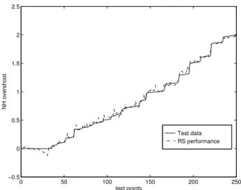
In Table 2, the values for the residuals show the average error for the response surface using the first data set. The error (av-erage modelling error) values are those for the validation set. Note that there are 10 RS models for the 10 responses (ob-jectives and constraints) required for design purposes. The design points are the actual values of these objectives and constraints the system achieves for the original controller at the chosen operating point. The steady-state errors and over-shoot of the variables were calculated taking into account the design specifications presented in Section 4. The optimiza-tion of the nozzle area (A8) steady-state (ss) was considered to maintain safer LPSM.
Table 2: Error performance values for the RS models
Output Mean Modelling Design residual error point Constraints
Thrust 0.0517 0.0730 48.6 kN TBT 2.4127 2.2526 1713 K XGN-rtime 0.0033 0.0049 1.0 s XGN-stime 0.0576 0.0897 1.4 s Objectives
LPSM 0.2907 0.4292 10 % NH ss error 0.0027 0.0060 0.095 NL ss error 0.0088 0.0164 0.18 A8 ss error 0.0010 0.0015 0 NH ov’shoot 0.0072 0.0126 0.47 NL ov’shoot 0.0181 0.0351 0.90
Test data RS performance
0 50 100 150 200 250
0 0.2 0.4 0.6 0.8 1
XGN
test points
Figure 2: Performance of the RS model predicting XGN out-put
6
USE OF RS IN MOGA-PI CONTROLLER
DESIGN
Once the RS models are established for this optimization problem, they are used for function evaluation within the MOGA instead of the non-linear SIMULINK engine model. The MOGA generates a set of 2 PI controller gains for the fuel flow and nozzle area loops. The designs created by the algorithm are then used to evaluate the response surface mod-els.
A MOGA using 80 individuals is evolved over 100 gener-ations to search for the best controller gains for the two PI controllers, satisfying the various objectives and constraints mentioned in Section 4. The controller parameters are
en-Test data RS performance
0 50 100 150 200 250
0 0.2 0.4 0.6 0.8 1
TBT
test points
Figure 3: Performance of the RS model predicting TBT out-put
Test data RS performance
0 50 100 150 200 250
0 0.5 1 1.5
LPSM
test points
Figure 4: Performance of the RS model predicting LPSM output
coded as 16-bit Gray-coded chromosome. Standard two-point crossover was used for recombination, and standard mutation was applied. All the objectives were assigned the same level of priority. All constraints were assumed to have the same level of priority. The actual evaluation time is lit-erally a few minutes of a standard workstation. The same scenario using the full model will require in excess of day to execute on the same machine.
7
RESULTS
Test data RS performance
0 50 100 150 200 250
−0.5 0 0.5 1 1.5 2 2.5
NH overshoot
test points
Figure 5: Performance of the RS model predicting NH over-shoot output
against time in seconds, and the response values are all nor-malized such that unity represents the desired response.
The MOGA finds a set of nondominated designs for the PI controllers. To reduce the size of this set, some of the ob-jectives are tightened further. It was chosen controllers with fastest responses in terms of thrust rise and settling times. It was also looked for controllers with minimum overshoot and good tracking performance in terms of steady state (ss) er-rors. These modified preferences reduce the number of con-trollers to a subset of similar gain ranges. The final designs for the PI controllers are validated using the full thermody-namic model. The actualy and predictedyˆvalues for the ten objective values are almost identical. Table 3 gives the percentage modelling error for the outputs given by:
δi= 100∗(|yˆi−yi|/ˆyi) (4)
fori= 1, ..., ne.
Table 3: RS design modelling errors (%)
Constraints Modelling Objectives Modelling
error error
Thrust 0.016 LPSM 0.01 TBT 0.3 NH ss error 0.001 XGN-rtime 0.4 NL ss error 0.0 XGN-stime 1.14 A8 ss error 0.0 NH ov’shoot 0.0 NL ov’shoot 0.0078
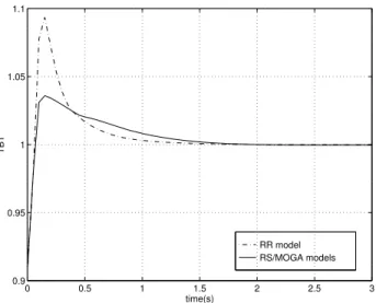
Figures 6-9 show fast and steady responses for the engine. The thrust response in particular is of great importance for
RR model RS/MOGA models
0 0.5 1 1.5 2 2.5 3
0.94 0.95 0.96 0.97 0.98 0.99 1 1.01
NH
time(s)
Figure 6: High-pressure spool speed
RR model RS/MOGA models
0 0.5 1 1.5 2 2.5 3
0.7 0.75 0.8 0.85 0.9 0.95 1 1.05
XGN
time(s)
Figure 7: Gross thrust
a military aircraft, both in terms of speed of response and attaining adequate thrust values. Turbine blade temperature is maintained within the allowable physical range avoiding deformation of the blades. In order to maintain a robust and stable engine operation, the surge margin has to be a mini-mum of 10%. In this case, a low pressure surge margin of nearly 14% is achieved and maintained, ensuring stall-free conditions.
RR model RS/MOGA models
0 0.5 1 1.5 2 2.5 3
0.9 0.95 1 1.05 1.1
TBT
time(s)
Figure 8: Turbine blade temperature
RR model RS/MOGA models
0 0.5 1 1.5 2 2.5 3
0.8 1 1.2 1.4 1.6 1.8 2
LPSM
time(s)
Figure 9: Low-pressure surge margin
8
CONCLUSIONS
A combination of both non-linear and linearized models, data-fitted approximations were used to design controllers for a gas turbine engine. The optimization was carried out using a MOGA. The designs found are shown to be good.
Variable complexity modelling techniques like the response surface models allow the designer the freedom to explore the design space more freely in search for the best design re-gions. Once near optimal designs are established this way, fine tuning can be carried out if necessary using the full mod-els.
The initial cost of establishing the RS models is more than offset by the savings in the design process. Further, these
models are re-usable at no extras cost. The construction of the models sheds more light on the design problem and helps design optimization in the process.
More complex data fitting techniques such as genetic pro-gramming or neural networks can be used, if it is needed. But, it can lessen the effect of simplicity of this approach. Least square polynomials are more than adequate for this problem.
REFERENCES
Balabanov, V., Kaufman, M., Knill, D.L., Haim, D., Golovi-dov, O., Giunta, A.A., Haftka, R.T., Grossman, B., Ma-son W.H., and WatMa-son, L.T., (1996),“Dependence of Optimal Structural Weight on Aerodynamic Shape for a High Speed Civil Transport”.Proceedings of the 6th AIAA/NASA/USAF Multidisciplinary Analysis and Op-timization Symposium, Bellevue, WA, 599-612. (AIAA Paper 96-4046)
Fonseca, C. M. and Fleming, P. J., 1993, “Genetic algorithms for multiobjective optimization: formulation, discus-sion and generalization,”In Genetic Algorithms: Pro-ceedings of the Fifth International Conference(S. For-rest, ed.), San Mateo, CA: Morgan Kaufmann.
Fonseca, C.M. and Fleming, P.J., (1995). “An overview of evolutionary algorithms in multiobjective optimiza-tion”.Evolutionary Computing. Vol. 3, N˚. 1, pp. 1-16.
Giannakoglou, K.C., (2002), “Design of optimal aerody-namic shapes using stochastic optimization methods and computational intelligence”,Progress in Aerospace Sciences, Vol. 38-1, pp. 43-76.
Giunta, A.A., Balabanov, V., Burgee, S., Grossman, B., Mason, W.H., Watson, L.T., and Haftka, R.T., (1996), “Parallel Variable-Complexity Response Sur-face Strategies for HSCT Design”,Proceedings of the NASA Ames Computational Aerosciences Workshop 95, Editors: Feiereisen, W.J. and Lacer, A.K., NASA CD Conference Publication 20010, Moffett Field, CA, 86-89.
Giunta, A.A., Balabanov, V., Kaufman, M.D., Burgee, S., Grossman, B., Haftka, R.T., Mason, W.H. and Wat-son, L.T., (1997), “Variable-Complexity Response Sur-face Design of an HSCT Configuration”,Proceedings of ICASE/LaRC Workshop on Multidisciplinary Design Optimization, SIAM, Philadelphia, PA, 348-367.
AIAA Applied Aerodynamics Conference, San Diego, CA, 19-22, 994-1002. (AIAA Paper 95-1886)
Goldberg, D.E., (1989). “Genetic algorithms in search, optimization and machine learning”. Reading, Mas-sachusetts: Addison-Wesley.
Khatib, W. & Fleming, P. J., (1997), “An introduction to evolutionary computing for multidisciplinary optimiza-tion”, Proceddings of GALESIA’97, Glasgow, UK, 7-12.
Mason, R.L., Gunst, R.F. and Hess, J.L., (1989). “Statistical design and analysis of experiments”. London, UK: John Wiley & Sons.
Myers, R.H. and Montgomery, D.C., (1995). “Response sur-face methodology. Process and product optimization using designed experiments”. London, UK: John Wi-ley & Sons.