DIRECT ADAPTIVE CONTROL USING FEEDFORWARD NEURAL
NETWORKS
Daniel Oliveira Cajueiro
∗Elder Moreira Hemerly
†∗Universidade Cat´olica de Bras´ılia, SGAN 916, M´odulo B – Asa Norte. Bras´ılia (DF) CEP: 70790-160
†Instituto Tecnol´ogico de Aeron´autica ITA-IEE-IEES, Pra¸ca Marechal Eduardo Gomes 50 – Vila das Ac´acias
S˜ao Jos´e dos Campos (SP) CEP: 12228-900
ABSTRACT
This paper proposes a new scheme for direct neural adaptive control that works efficiently employing only one neural network, used for simultaneously identifying and controlling the plant. The idea behind this struc-ture of adaptive control is to compensate the control input obtained by a conventional feedback controller. The neural network training process is carried out by using two different techniques: backpropagation and ex-tended Kalman filter algorithm. Additionally, the con-vergence of the identification error is investigated by Lyapunov’s second method. The performance of the proposed scheme is evaluated via simulations and a real time application.
KEYWORDS: Adaptive control, backpropagation, con-vergence, extended Kalman filter, neural networks, sta-bility.
RESUMO
Este artigo prop˜oe uma nova estrat´egia de controle
adaptativo direto em que uma ´unica rede neural ´e
usada para simultaneamente identificar e controlar uma planta. A motiva¸c˜ao para essa estrat´egia de controle
Artigo submetido em 23/11/2000
1a. Revis˜ao em 15/10/2001; 2a. Revis˜ao 3/7/2003
Aceito sob recomenda¸c˜ao dos Eds. Associados Profs. Fernando
Gomide e Ricardo Tanscheit
adaptativo ´e compensar a entrada de controle gerada por um controlador retroalimentado convencional. O processo de treinamento da rede neural ´e realizado
atra-v´es de duas t´ecnicas: backpropagatione filtro de Kalman
estendido. Adicionalmente, a convergˆencia do erro de identifica¸c˜ao ´e analisada atrav´es do segundo m´etodo de Lyapunov. O desempenho da estrat´egia proposta ´e ava-liado atrav´es de simula¸c˜oes e uma aplica¸c˜ao em tempo real.
PALAVRAS-CHAVE: Backpropagation, controle adapta-tivo, convergˆencia, estabilidade, filtro de Kalman esten-dido, redes neurais.
1
INTRODUCTION
Different neural networks topologies have been intensi-vely trained aiming at control and identification of non-linear plants (Agarwal, 1997; Hunt et al., 1992). The neural networks usage in this area is explained mainly by their following capability: flexible structure to model and learn nonlinear systems behavior (Cibenko, 1989). In general, two neural networks topologies are used: fe-edforward neural networks combined with tapped delays (Hemerly and Nascimento, 1999; Tsuji et al., 1998) and recurrent neural networks (Sivakumar et al., 1999; Ku and Lee, 1995). The neural network used here belongs to the former topology.
simultane-ously identifying and controlling the plant and the un-certainty can be explicitly identified. The idea behind this approach of direct adaptive control is to compen-sate the control input obtained by a conventional feed-back controller. A conventional controller is designed by employing a nominal model of the plant. Since the nominal model may not match the real plant, the perfor-mance of the nominal controller previously designed will not be adequate in general. Thus the neural network, arranged in parallel with the feedback conventional con-troller, identifies the uncertainty explicitly and provides the control signal correction so as to enforce adequate tracking.
For some other neural direct adaptive control schemes the neural network is placed in parallel with the feedback conventional controller as has been presented (Kraft and
Campanha, 1990; Kawatoet al., 1987). The scheme
pro-posed here differs from these results, in the sense that the neural network aim at improving and not replacing the nominal controller. Additionally, Lightbody and Irwin (1995) proposed a neural adaptive control scheme where the neural network is arranged in parallel with a fixed gain linear controller. The main difficult of this scheme is to update the neural network weights by using the error calculated between the real plant and the refe-rence, in other words, the problem known as backpropa-gation through the plant (Zurada, 1992). In this case, the convergence of the neural network identification er-ror to zero is often more difficult to be achieved (Cui and Shin, 1993). This problem does not appear here.
Although our approach is similar to that used by Tsuji et al. (1998), it has three main advantages (Cajueiro, 2000): (a) while their method demands modification in the weight updating equations which is computationally more complicated, our training procedure can be perfor-med by a conventional feedforward algorithm; (b) while their paper presents a local asymptotic stability analysis of the parametric error for the neural network trained by backpropagation algorithm where the nominal mo-del must be SPR, that analysis can also be applied to our scheme without this condition; (c) their scheme can be only applied for plants with stable nominal model, which is not the case here.
This paper is organized as follows. In section 2, the con-trol scheme and the model of the plant are introduced. In section 3 the model of the neural network is descri-bed and in section 4 the convergence of the NN based adaptive control is investigated. In section 5 some si-mulations are conducted. Finally, in section 6 a real time application is presented. Section 7 deals with the conclusion of this work.
2
PLANT MODEL AND THE
PROPO-SED ADAPTIVE CONTROL SCHEME
2.1
Plant Model with Multiplicative
Uncer-tainties
We firstly consider the case in which the controlled plant presents multiplicative uncertainty (Maciejowski, 1989). Consider the SISO plant
y(k) =G(z−1)u(k) (1)
LetGn(z−1) be the nominal model and ∆Gm(z−1) the
multiplicative uncertainty, i.e.,
G(z−1) =G
n(z−1)[1 + ∆Gm(z−1)] (2)
whereGn(z−1) and ∆Gm(z−1) are given as
Gn(z−1) =
Bn(z−1)
An(z−1)
(3)
beingBn(z−1) is Hurwitz,
∆Gm(z−1) =
∆Bm(z−1)
∆Am(z−1)
(4)
2.2
Proposed Adaptive Control Scheme
We start by designing the usual feedback control system.
If there is no uncertainty, i.e., ∆Gm(z−1) = 0 in (2),
then the nominal feedback controller Cn(z−1) can be
designed to produce the desirable performance.
Now, let us consider the general case in which
∆Gm(z−1) = 0. Hence the controller must be
modi-fied accordingly, i. e.,
C(z−1)=∆C
n(z−1)[1 + ∆Cm(z−1)] (5)
It is easy to prove that
∆Cm(z−1) =−
∆Gm(z−1)
1 + ∆Gm(z−1)
(6)
is the controller correction necessary to enforce the de-sired performance (Tsuji et al., 1998).
However, ∆Gm(z−1) is unknown, hence ∆Cm(z−1) can
not be calculated in (6), and then the controller (5) is not directly implementable. In order to circumvent this dif-ficulty, we propose the NN based scheme for identifying
1
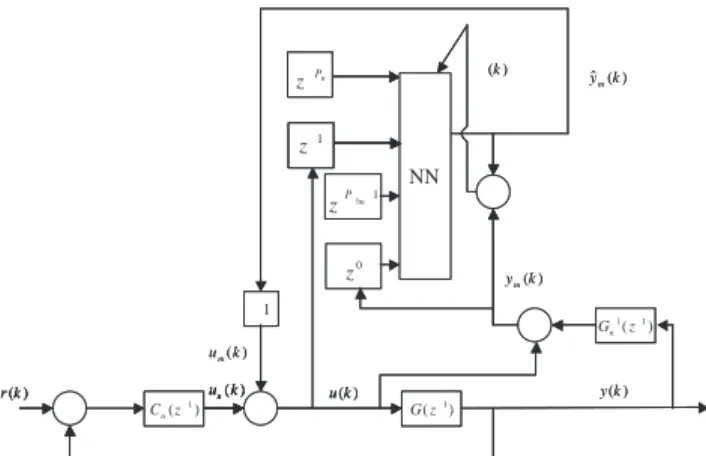
)
(k ˆy(k)
m ) (k ym ) ( 1 1z Gn ) (k um ) (k y ) (k u ) (z1
G ) (k un ) (k r NN ) (z1
Cn NN 0 z u P z 1 z 1 my P z 1 1 )
(k ˆy(k)
m ) (k ym ) ( 1 1z
Gn( ) 1 1z Gn ) (k um ) (k y ) (k u(k) u
) (z1
G(z1) G )
(k un(k)
un(k)
un
) (k r(k) r
NN
) (z1
Cn( ) 1 z Cn NN 0 z u P z 1 z u P
zPu
zPu
z 1 z1 z1 z 1 my P z
Figura 1: Block diagram of the proposed NN based adaptive control scheme.
Definition 1: yn(k), the output of the nominal model,
is given by
yn(k) =Gn(z−1)u(k) (7)
Definition 2: ∆ym(k), the filtered mismatch between
the plant output and its nominal model output denoted
byy(k) andyn(k) respectively, is given by
∆ym(k)
∆
=∆Gm(z−1)u(k)
=G−1
n (z−1)·(y(k)−yn(k))
=G−n1(z−1)·y(k)−u(k) (8)
Definition 3: u(k), the control input, from (5) can be written as
u(k) =Cn(z−1)[1 + ∆Cm(z−1)]e(k)
∆
=un(k) + ∆um(k)
(9)
where
un(k) =Cn(z−1)e(k) (10)
is the nominal control signal and
∆um(k) = ∆Cm(z−1)un(k) (11)
is the control signal modification.
Definition 4: ε(k), the identification error, is given by
ε(k) = ∆ym(k)−∆ˆym(k) (12)
From (1), (2), (7) and (8) the output of the plant is given by
y(k) =Gn(z−1)[1 + ∆Gm(z−1)]u(k)
=yn(k) +Gn(z−1)∆ym(k) (13)
Now, from (9) and (13) we get
∆ym(k) =∆Gm(z−1)[un(k) + ∆um(k)]
=∆Gm(z−1)[1 + ∆Cm(k)]un(k) (14)
and from (9) and (14), the control signal correction
∆um(k) can be rewritten as
∆um(k) =
∆Cm(z−1)
∆Gm(z−1)[1 + ∆Cm(z−1)]
∆ym(k) (15)
By replacing (6) into (15), we obtain
∆um(k) =−∆ym(k) (16)
Moreover, ifε →0, from equations (12) and (16) then
∆ˆym(k) = ∆ym(k) =−∆um(k).
On the other hand, from equations (1), (2), (8) and (16), one should write
y(k) =yn(k) +Gn(z−1)∆ym(k)
=Gn(z−1)(un(k) + ∆um(k)) +Gn(z−1)∆ym(k)
=Gn(z−1)(un(k)−∆ym(k)) +Gn(z−1)∆ym(k)
=Gn(z−1)un(k) (17)
Remark 1: It is clear from (17) that if ε → 0 then the control scheme will behave as desired. Therefore, from (10) it is obvious that the nominal controller signal converges to the nominal controller signal obtained by controlling the nominal plant.
Remark 2: The neural network here is a direct model
of the uncertainty ∆Gm(z−1) and is aiming at
approxi-mating the uncertainty output ∆ym(k).
Remark 3: In spite of the nominal model minimum phase restriction this scheme of adaptive control can also be applied to non-minimum phase systems. It depends on the neural network ability for identifying the uncer-tainty arising from a non-minimum phase plant modeled by a minimum phase nominal model.
Remark 4: Although this neural adaptive control scheme is developed to compensate the nominal con-troller signal of plants with multiplicative uncertainty, it also can compensate other type of non structured un-certainty. Consider, for instance, the additive case
G(z−1) =Gn(z−1) + ∆Ga(z−1) (18)
On the other hand, although equations (16) and (17) can only be applied for linear plants, this scheme of neural adaptive control also presents good performance when applied for nonlinear plants (Cajueiro and He-merly, 2000).
3
NEURAL NETWORK TOPOLOGY
The neural network topology used here is a feedforward one combined with tapped delays. The training process is carried out by using two different techniques: back-propagation and extended Kalman filter. The two ap-proaches used to train the neural network are justified due to the slow nature of the training with the standard backpropagation algorithm (Sima, 1996; Jacobs, 1988). Thus the neural network trained via extended Kalman filter can be useful in more difficult problems.
The input of the neural network is defined as follows
ΦI(k) = [ u(k−1) · · · u(k−Pu )
∆ym(k−1) · · · ∆ym(k−P∆ym) ]
T (19)
where ∆ym(k−1) . . . ∆ym(k−P∆ym) is
calcula-ted by using (8) and the cost function is defined, from (12) as
J(k) = 1 2ε(k)
2=1
2(∆ym(k)−∆ˆym(k))
2 (20)
3.1
Learning Algorithm Based on the
Ex-tended Kalman Filter
The Kalman filter approach for training a multilayer perceptron considers the optimal weights of the neural network as the state of the system to be estimated and the output of the neural network as the associated mea-surement. The optimal weights are those that minimize
the costJ(k). The weights are in general supposed to be
constant, and the problem boils down to a static estima-tion problem. However, it is often advantageous to add some noise, which prevents the gain from decreasing to zero and then forces the filter to continuously adjusting the weight estimates. Therefore, we model the weights as
w(k+ 1) =w(k) +vw(k),
E[vw(i)vw(j)T] =Pvwδ(i−j) (21)
The measurements of the system are assumed to be some nonlinear function of the states corrupted by zero-mean white Gaussian noise. Thus, the observations of the
system are modeled as
ΦO(k) =h(w(k),ΦI(k)) +v
ΦO(k)E[vΦO(i)vΦO(j)T]
=PΦOδ(i−j), (22)
The extended Kalman filter equations associated to pro-blem (19) and (20) are (Singhal and Wu, 1991)
ˆ
w(k+ 1) = ˆw(k) +K(k)ε(k) (23)
P(k+ 1) =P(k)−K(k)H(k)P(k) +Pvw (24)
whereK(k) is the Kalman filter gain given by
K(k) =P(k)H(k)T[H(k)P(k)H(k)T +P vΦO]
−1 (25)
with
H(k) =
∂ΦO(k)
∂w(k)
T
w(k) = ˆw(k) (26)
There are some local approaches (Iiguni et al., 1992; Shah et al., 1992) for implementing the extended Kal-man filter to train neural networks in order to reduce the computational cost of training. Since we are using small neural networks, this is not an issue here. Then, we consider only the global extended Kalman algorithm, more precisely, the approach known by GEKA - Global Extended Kalman Algorithm (Shah et al., 1992).
3.2
The Standard Backpropagation
Algo-rithm
The standard backpropagation algorithm is a gradi-ent descgradi-ent method for training weights in a multilayer preceptron that was popularized by Rumelhart et al. (1986). The basic equation for updating the weights is
∆ ˆw(k) =−ηε(k)∂J(k)
∂wˆ(k) =ηε(k)
∂ΦˆO(k)
∂wˆ(k) (27)
From (23) – (26), it can be seen that the extended Kman filter algorithm reduces to the backpropagation al-gorithm when
[H(k)P(k)H(k)T +P
v]−1=aI (28)
P(k) =pI (29)
andηis given by
η =p·a (30)
4
STABILITY
AND
CONVERGENCE
ANALYSIS
The stability analysis is divided into two parts: (a) the study of the influence of the neural network in the con-trol system stability when the nominal concon-troller em-ployed to control the real plant is analyzed; (b) the inves-tigation of the conditions under which the identification error of the neural network asymptotically converges to zero are investigated.
4.1
Control System Stability
The closed loop equation that represents the control sys-tem shown in Fig.1, without considering the dynamics uncertainty and the output of the neural network, is
y(k) = Gn(z
−1)C
n(z−1)
1 +Gn(z−1)Cn(z−1)
r(k) (31)
It represents a stable system, sinceCn(z−1) is properly
designed.
By considering now the introduction of the uncertainties and the control signal correction via NN, from Fig. 1 we get
y(k) = (1 + ∆Gm(z
−1))G
n(z−1)
1 + (1 + ∆Gm(z−1))Gn(z−1)Cn(z−1)
ˆ
ΦO(k)+
(1 + ∆Gm(z−1))Gn(z−1)Cn(z−1)
1 + (1 + ∆Gm(z−1))Gn(z−1)Cn(z−1)
r(k) (32)
Since ˆΦO(k) = tanh(•), where tanh(•) is the
hyperbo-lic tangent function, andr(k) are bounded, in order to
guarantee the stability we have to analyze under which conditions the denominator of (32) is a Hurwitz poly-nomial, when the denominator of (31) also is. These conditions can be found in a very general result, known as the small gain theorem, which states that a feedback loop composed of stable operators will certainly remain stable if the product of all the operator gains is smaller than unity. Therefore, if a multiplicative perturbation satisfies the conditions imposed by the small gain
theo-rem, then one should assert thatε(k), given by equation
(12), is bounded. Since ˆΦH(k) and ˆΦO(k), the output of
the neural network layers, depend on the weights whose
boundedness depends on the boundedness ofε(k), it is
clear that the boundedness ofε(k) is the first condition
for the output of the neural network layers, ˆΦH(k) and
ˆ
ΦO(k), not saturating. If saturation happens, then in
(26)H(k) = 0 and we can not conclude, as in section
4.2, that the identification error converges asymptoti-cally to zero.
4.2
Identification Error Convergence
We start by analyzing the conditions under which the neural network trained by Kalman filter algorithm gua-rantees the asymptotic convergence of the identification error to zero. Next, we show that a similar result is va-lid for the neural network trained by backpropagation algorithm.
Theorem 1: Consider that the weightsw(k) of a mul-tilayer perceptron are adjusted by the extended Kalman
algorithm. If w(k)∈ L∞, then the identification error
ε(k) converges locally asymptotically to zero.
Proof:
LetV(k) be the Lyapunov function candidate, which is
positive definite, given by
V(k) = 1
2ε
2(k) (33)
Then, the change ofV(k) due to training process is
ob-tained by
∆V(k) = 1
2[ε
2(k+ 1)−ε2(k)] (34)
On the other hand, the identification error difference due to the learning process can be represented locally by (Yabuta and Yamada, 1991)
∆ε(k) =
∂ε(k)
∂wˆ(k)
T
∆ ˆw(k) =
∂ΦˆO(k)
∂wˆ(k)
T
∆ ˆw(k) (35)
From equations (21) and (33),
∆ε(k) =−
∂ΦˆO(k)
∂wˆ(k)
T
∆ ˆw(k) =
−H(k)K(k)ε(k) =−QEKFε(k) (36)
where
QEKF(k)
∆
=H(k)K(k) (37)
and it can be easily seen that 0 QEKF(k) < 1 and
then, from (32) and (34),
∆V(k) = 2ε(k)∆ε(k) + ∆ε2(k) =
−ε2(k)(2QEKF(k)−Q2EKF(k)) (38)
From (38) follows that for asymptotic convergence of
(37) a sufficient condition for this is H(k) = 0. On the other hand, (26) implies this only occurs when the weights are bounded. However, this can not be proved to happen, since the Lyapunov candidate function does not explicitly include the weight error. This depends on the proper choice of the neural network size and initial parameters. Hence, we have to assume that the neural network size and initial parameters have been properly selected. This difficulty is also present, although disgui-sed, in Ku and Lee (1995) and Liang (1997).
Corollary 1: Consider that the weightsw(k) of a mul-tilayer perceptron are adjusted by the backpropagation
algorithm. Ifw(k)∈L∞and 0< η < 2
∂ΦO(k) ∂w(k)
2 , where
ΦO(k) is the output of the neural network, then the
iden-tification errorε(k) converges locally asymptotically to
zero.
Proof:
The convergence of the identification error of a neural network trained by backpropagation algorithm is a spe-cial case of the above result. More precisely, by consi-dering equations (25), (28) - (30), one can arrive at an equation similar to (37), with
QBP(k)
∆
=η
∂ΦO(k)
∂w(k)
2
(39)
and the correspondent variation inV(k) is
∆V(k) =−ε2(k)(2QBP(k)−Q2BP(k)) (40)
Equation (40) states that the convergence of the identi-fication error for the neural network trained by
backpro-pagation method is guaranteed as long as
∂ΦO
(k)
∂w(k)
= 0
, and
0< η < 2
∂ΦO(k)
∂w(k)
2 (41)
so as to enforce ∆V(k)<0 in (40) when ε(k)= 0.
Remark 5: Although (38) and (40) have the same form, the conditions for the identification error conver-gence are more restrictive when the backpropagation al-gorithm is used, since an upper bound in the learning rate is required, given by (41), as we should have expec-ted.
Remark 6: Since the candidate Lyapunov function gi-ven by equation (33) does not include the parametric
error ˜w(k) = w∗(k)−wˆ(k), even if there were an
opti-mal set of parameters, the convergence of ˜w(k) to zero
would depend on the signal persistence.
Remark 7: Since (40) is a quadratic equation, a bigger
learning rate η does not imply that there is a faster
learning.
5
SIMULATIONS
In this section, simulations of two different plants are presented to test the proposed control scheme. We start by considering a linear plant to which can be applied equations (16) and (17). Next, a non-BIBO nonlinear plant is used as a test. Moreover, the stability of this control system can not be assured, since the nominal controller designed by using the nominal model results in an unstable control scheme when it is applied to the real plant.
5.1
Simulation with Linear Plant
The plant used here has the nominal model given by
Gn(z−1) =
0.01752z−1+ 0.01534z−2
1−1.637z−1+ 0.6703z−2 (42)
and it is considered the following multiplicative uncer-tainty
∆Gm(z−1) =
0.1848z−1
1−0.8521z−1 (43)
Thus, from equations (2), (42) and (43), one should write the model of the real plant
G(z−1) = 0.01752z−1+ 0.003642z−2−0.01023z−3
1−2.49z−1+ 2.066z−2−0.5712z−3
(44)
The nominal controller here is given by
un(k) =un(k−1) +Kp(e(k)−e(k−1)) +KIe(k)
(45)
withKp= 2.0 andKI = 0.26.
As it can be seen in Fig. 2, although the control system presents good performance when nominal controller is applied to the nominal model, the control system is too oscillatory when the nominal controller is applied to the real plant.
The input of the neural network is
ΦI(k) =
u(k−1) ∆ym(k−1)
(46)
The initial weights were initialized within the range
−0.1 0.1
100 200 300 400 500 600 700 800 -1.5
-1 -0.5 0 0.5 1
Time steps
Control system outputs
Nominal model / Nominal Controller Real plant / Nominal controller
Figura 2: Control systems performance using the nomi-nal controller
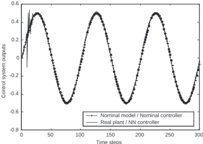
usual backpropagation. The usage of the algorithm ba-sed on the extended Kalman filter is not justified since the neural network task here is simple. Fig. 3 shows the output of the nominal model and the output of the real plant controlled by the proposed scheme using the back-propagation algorithm, after few time steps an adequate performance is achieved.
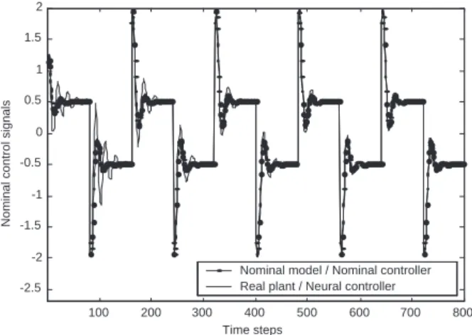
Fig. 4 shows that the nominal controller signal conver-ges to the nominal controller signal that would exist if there was no uncertainty.
Remark 8: Since the plant given by (44) is linear, one should note that the uncertainty could be identified by using a linear neural network or a least squares and an ARX model. This will not occur in section 5.2.
5.2
Simulations with a Non-BIBO
Nonli-near Plant
The nonlinear plant used to test the proposed method is the one given by Ku and Lee (1995), that is, a non-BIBO nonlinear plant, linear in the input.
The reference signal is given by
r(k+ 1) = 0.6r(k) +βsin(2πk/100) (47)
whereβ= 0.2, and the real plant is given by
y(k+ 1) = 0.2y2(k) + 0.2y(k−1) + 0.4 sin[0.5(y(k)+
y(k−1))]·cos[0.5(y(k) +y(k−1))] + 1.2u(k) (48)
This plant is unstable in the sense that given a sequence
of uniformly bounded controls{u(k)}, the plant output
100 200 300 400 500 600 700 800 -1
-0.8 -0.6 -0.4 -0.2 0 0.2 0.4 0.6 0.8 1
Time steps
Control system outputs
Nominal model / Nominal controller Real plant / Neural controller
Figura 3: Performance of the real plant controlled by the proposed scheme using the backpropagation algorithm.
100 200 300 400 500 600 700 800 -2.5
-2 -1.5 -1 -0.5 0 0.5 1 1.5 2
Time steps
Nominal control signals
Nominal model / Nominal controller Real plant / Neural controller
Figura 4: Nominal control signals.
may diverge. The plant output diverges when the step
inputu(k)0.83, ∀kis applied.
Ku and Lee (1995) employed two DRNNs (Diagonal Re-current Neural Networks), one as an identifier and the other as the controller, and an approach based on adap-tive learning rates to control this system. Their neu-ral network used as identifier employed 25 neurons and the one used as controller had 42. Here, we use the scheme proposed in section 2: the nominal model is that identified by employing an ARX model, and the neural network for simultaneous control and identification, has 21 neurons. Although our approach is much simpler and less computationally expensive than that in Ku and Lee (1995) and it produces better results.
Squa-res and ARX model, thereby Squa-resulting
Gn(z−1) =
1.2134z−1−0.6124z−2
1−0.9061z−1+ 0.1356z−2 (49)
In this simulation, the nominal controller used is a proportional-integral controller, given by (45) with
Kp=KI = 0.5.
The control system employing the nominal controller for controlling the real plant (48) results unstable, although the nominal controller provides good tracking of the re-ference signal (47) when applied to the nominal model (49).
The input of the neural network here is also given by (46).
The initial weights were randomly initialized in the
range [−0.1,0.1]. The simulations were performed by
usual backpropagation and extended Kalman filter using the same conditions and the same seed for generating the initial weights. The learning rate used in the first case
wasη = 1 and the initial data for the second case was
P(0) = 100I,PΦO =Pw= 10−5.
In Fig. 5, the output of the nominal model controlled by the nominal controller and the output of the real plant controlled by the proposed scheme using the backpropa-gation algorithm are presented. After a hundred time steps, the control system exhibits adequate tracking.
Fig. 6 shows the control system outputs when the tended Kalman filter algorithm is used. Since the ex-tended Kalman filter uses the information contained in the data more efficiently, the convergence is much faster than that in Fig. 5.
It should be highlighted here that the speed of conver-gence in Figs. 5 and 6 is more than 10 times faster than that reported in (Ku and Lee, 1995).
Remark 9: A comparison between the algorithm based on the extended Kalman filter and the backpropagation algorithms can be done as follows: (a) The algorithm based on the extended Kalman Filter presents better transient performance, but it is computationally more expensive; (b) the algorithm based on the extended Kal-man filter has presented more sensibility to the choice of
its parametersP(0), PΦO and Pw than the
backpropa-gation algorithm for the choice of its only one parameter
η.
0 50 100 150 200 250 300
-1 -0.5 0 0.5 1 1.5
Time steps
Control system outputs
Nominal model / Nominal controller Real plant / NN controller
Figura 5: Simulation of a nonlinear non-BIBO plant using backpropagation algorithm.
0 50 100 150 200 250 300
-0.8 -0.6 -0.4 -0.2 0 0.2 0.4 0.6
Time steps
Control system outputs
Nominal model / Nominal controller Real plant / NN controller
Figura 6: Simulation of a nonlinear non-BIBO plant using extended Kalman filter algorithm.
6
REAL TIME APPLICATION
The real time application employs the Feedback Process Trainer PT326, shown in Fig. 7, and the scheme pro-posed in section 2. This process is a thermal process in which air is fanned through a polystyrene tube and heated at the inlet, by a mesh of resistor wires. The air temperature is measured by a thermocouple at the outlet.
The nominal model used was identified using Least Squares with ARX model, as in Hemerly (1991), and is given by
Gn(z−1) =
0.0523
Thermocouple Wires
Resistor (Inlet)
Air Cold
) (k
u y(k)
Polystyrene Tube
Hot Air (Outlet )
Figura 7: Set up for real time control of the thermal process PT326.
0 50 100 150 200 250
0 0.2 0.4 0.6 0.8 1 1.2 1.4
Time steps
Control system outputs
Nominal model / Nominal controller Real plant / Nominal controller
Figura 8: Control system performance using the nomi-nal controller.
The nominal controller is a proportional-integral
con-troller withKP = 1 andKI = 1, given by the equation
(45). The input of the neural network is the same as in (46). The neural network used here is trained using the backpropagation method. The remaining design
pa-rameters are sampling time 0.3s, learning rateη= 0.05
and the initial weights randomly in the range [−0.1,0.1].
As can be seen in Fig. 8, the nominal controller is such that the control system presents a too oscillatory beha-vior. Hence, the introduction of the neural network is well justified.
In Fig. 9 we can see that the NN controller compen-sates for the uncertainty, and adequate performance is achieved after few time steps.
7
CONCLUSIONS
This paper proposed a neural adaptive control scheme useful for controlling linear and nonlinear plants (Caju-eiro, 2000; Cajueiro and Hemerly, 2000), using only one
0 50 100 150 200 250
0 0.2 0.4 0.6 0.8 1 1.2 1.4
Time steps
Control system outputs
Nominal model / Nominal controller Real plant / NN controller
Figura 9: Control system performance using the NN based proposed scheme.
neural network which is simultaneously applied for con-trol and identification. The nominal model can either be available or identified at low cost, for instance by using the Least Squares algorithm. The identification perfor-med by the neural network is necessary only to deal with the dynamics not encapsulated in the nominal model. If the proposed scheme is compared to another schemes, one should consider the following: (a) The approaches which try to identify the whole plant dynamics can have poor transient performance. For instance, in Ku and Lee (1995) the plant described by (48) is identified and more than three thousand time steps are required. (b) The neural network control based methods that need to iden-tify the inverse plant have additional problems. (c) If more than one neural network has to be used, in general the convergence of the control scheme is slow and the neural network tuning is usually difficult. (d) The ap-proaches that have to backpropagate the neural network identification error through the plant are likely to have problems to update the neural network weights.
When compared to Tsuji et al. (1998), the proposed scheme requires less stringent assumptions. In their lo-cal stability analysis the SPR condition is required for the nominal model. Moreover, we can employ an usual feedforward neural network, which is computationally less expensive than the one used there. Besides the scheme proposed here can also be applied to unstable plants. Additionally, here the asymptotic convergence of the identification error is analyzed for two different training algorithms.
ACKNOWLEDGEMENTS
This work was sponsored by Funda¸c˜ao CAPES - Co-miss˜ao de Aperfei¸coamento de Pessoal de N´ıvel Supe-rior and CNPQ-Conselho Nacional de Desenvolvimento Cient´ıfico e Tecnol´ogico, under grant 300158/95-5(RN).
REFERˆ
ENCIAS
Agarwal, M. (1997) A systematic classification of neural network based control, Control Systems Magazine, April, Vol. 17, No. 2, pp. 75-93.
Cajueiro, D. O. (2000) Controle adaptativo paralelo usando redes neurais com identifica¸c˜ao expl´ıcita da
dinˆamica n˜ao modelada. Master Thesis, Instituto
Tecnol´ogico de Aeron´autica, ITA-IEEE-IEES.
Cajueiro, D. O. and Hemerly, E. M. (2000) A chemi-cal reactor benchmark for parallel adaptive control using feedforward neural networks. Brazilian Sym-posium of Neural Networks, Rio de Janeiro.
Cibenko, G. (1989). Approximation by superpositions of a sigmoidal function, Mathematics of Control, Signals and Systems, Vol. 2, pp. 303-314.
Cui, X. and Shin, K. (1997) Direct control and coordi-nation using neural networks. IEEE Transactions on Systems, man and Cybernetics, Vol. 23, No. 3, pp. 686-697.
Hemerly, E. M. (1991). PC-based packages for identi-fication, optimization and adaptive control, IEEE Control Systems Magazine, Vol. 11, No. 2, pp. 37-43.
Hemerly, E. M. and Nascimento Jr., C. L. (1999). A NN-based approach for tuning servocontrollers, Neural Networks, Vol. 12, No. 3, pp. 113-118.
Hunt et al. (1992) Neural networks for control systems – a survey, Automatica, Vol. 28, No. 6, pp. 1083-1112.
Iiguni, Y., Sakai, H. and Tokumaru, H. (1992) A real time algorithm for a multilayered neural network based on the extended Kalman algorithm, IEEE Transactions on Signal Processing, Vol. 40, No. 4, pp. 959-966.
Jacobs, R. (1988). Increased rates of convergence th-rough learning rate adaptation, Neural Networks, Vol. 1, pp. 295-307.
Kawato, M. Furukawa, K. and Suzuki, R. (1987) A hi-erarchical neural network model for control and le-arning of voluntary movement, Biological Cyberne-tics, Vol. 57, No. 6, pp. 169-185.
Kraft, L. G. and Campagna, D. S. A. (1990) A summary comparison of CMAC neural network and two tra-ditional adaptive control systems, In: T. W. Miller III, R. S. Sutton, P. J. Werbos, Neural Networks for control. Cambridge: The MIT Press, pp. 143-169.
Ku, C. C. and Lee, K. Y. (1995). Diagonal recurrent neural networks for dynamic systems control, IEEE Transactions on Neural Networks, Vol. 6, No. 1, pp. 144-156.
Liang, X. (1997). Comments on “Diagonal recurrent neural networks for dynamic systems control” – Re-proof of theorems 2 and 4, IEEE Transactions on Neural Networks, Vol. 8, No. 3, pp. 811-812.
Lightbody, G. and Irwin, G. (1995) Direct neural mo-del reference adaptive control. IEE Proceedings in Control Theory and Applications, Vol. 142, No. 1, pp. 31-43.
Maciejowski, J. M. (1989) Multivariable feedback de-sign. Addison-Wesley Publishing Company.
Ruck, D. W. et al. (1992). Comparative analysis of back-propagation and the extended Kalman filter for training multilayer perceptrons, IEEE Transactions on Pattern Analysis and Machine Intelligence, Vol. 14, No. 6, pp. 686-691.
Rumelhart, D. E., Mcclelland, J. L. and Williams, R. J. (1986). Learning representations by error pro-pagation. In D. E. Rumelhart, G.E. Hilton, J. L. Mcclelland (Eds.), Parallel Distributed Processing, Vol. 1, pp. 318-362. Cambridge,MA: MIT Press.
Shah, S., Palmieri, F. and Datun, M. (1992). Optimal filtering algorithms for fast learning in feedforward neural networks, Neural Networks, Vol. 5, pp. 779-787.
Sima, J. (1996) Back-propagation is not efficient, Neural Networks, Vol. 9, No. 6, pp. 1017-1023.
Singhal, S. and Wu, L. (1991) Training feed-forward networks with the extended Kalman algorithm, Proceedings of the IEEE International Conference on Acoustics, Speech and Signal Peocessing, pp. 1187-1190.
Tsuji, T. , Xu, B. H. and Kaneko, M. (1998). Adaptive control and identification using one neural network for a class of plants with uncertainties, IEEE Tran-sactions on Systems, Man and Cybernetics – Part A: Systems and Humans, Vol. 28, No. 4, pp. 496-505.
Yabuta, T. and Yamada, T. (1991). Learning control using neural networks, Proceedings of the 1991 IEEE International Conference on Robotics and Automation, California, pp. 740-745.