ISSN 0101-8205 www.scielo.br/cam
A global linearization approach to solve nonlinear
nonsmooth constrained programming problems
A.M. VAZIRI1, A.V. KAMYAD1, A. JAJARMI2 and S. EFFATI1
1Department of Applied Mathematics, Ferdowsi University of Mashhad, Mashhad, Iran 2Department of Electrical Engineering, Ferdowsi University of Mashhad, Mashhad, Iran
E-mails: [email protected] / [email protected] / [email protected] / [email protected]
Abstract. In this paper we introduce a new approach to solve constrained nonlinear non-smooth programming problems with any desirable accuracy even when the objective function is a non-smooth one. In this approach for any given desirable accuracy, all the nonlinear functions of original problem (in objective function and in constraints) are approximated by a piecewise linear functions. We then represent an efficient algorithm to find the global solution of the later problem. The obtained solution has desirable accuracy and the error is completely controllable. One of the main advantages of our approach is that the approach can be extended to problems with non-smooth structure by introducing a novel definition of Global Weak Differentiation in the sense ofL1norm. Finally some numerical examples are given to show the efficiency of the proposed approach to solve approximately constraints nonlinear non-smooth programming problems.
Mathematical subject classification: 90C30, 49M37, 49M25.
Key words: nonlinear programming problem, non-smooth analysis, equicontinuity, uniform continuity.
1 Introduction
Frequently practitioners need to solve global optimization problem in many fields such as engineering design, molecular biology, neural network training and so-cial science. So that the global optimization becomes a popular computational
task for researchers and practitioners. There are some interesting recent papers for solving nonlinear programming problems [3], non-smooth global optimiza-tion [6, 10], solving a class of non-differentiable programming based on neural network method [11] and controllability for time-varying systems [4].
One of the efficient approaches for solving nonlinear programming problems is to linearize the nonlinear functions when the domain of the function is parti-tioned to very small sub-domains. However many realistic problems cannot be adequately linearized. So throughout its domain efforts to approximate nonlinear problems efficiently is the focused of the new researcher. Two other aspects that should be considered are non-convexity and non-smooth dynamics due to our ability to obtain the global solution of nonlinear, non-convex and non-smooth problems(when they exist) is still limited. So an efficient approach which is applicable in the presence of non-convex and non-smooth functions should be investigated (see [1, 2, 5]).
In this paper we introduce a new approach to solve approximately nonlinear non-smooth programming problems which don’t have any limitation upon con-vexity and smoothness of the nonlinear functions. In this approach any given nonlinear function is approximated by a piecewise linear function with controlled error. In this manner, the difference between global solution of the approximated problem and the main problem is less than or equal a desirable upper bound which is shown byε >0. Also we represent an efficient algorithm to find global solu-tion of approximated problem. One of the main advantages of our approach is that it can be extended to problems with non-smooth functions by introducing a novel definition of Global Weak Differentiation in the sense ofL1-norm. The paper is organized as follow:
2 Proposed approach for one dimensional problem
Consider the following non-constrained nonlinear minimization problem:
Minimize f(x) (1)
subject to x ∈ [a,b]
where f : [a,b] −→ R; is a nonlinear smooth function. We may approximate the nonlinear function f(x)by a piecewise linear function defined on [a,b]. Let us mention the following definitions.
Definition 2.1.Let Pn([a,b])be a partition of the interval[a,b]as the form:
Pn([a,b])=
a=x0,x1,∙ ∙ ∙ ,xn=b
whereh= b−na andxi =x0+i h. The norm of partition defined by:
kPn([a,b])k = max
1≤i≤n
xi−xi−1 . (2)
It is easy to show thatkPn([a,b])k →0 asn → ∞.
Definition 2.2.The function fi(x,si)is defined as follows:
fi(x,si), f′(si)x + f(si)−si f′(si); x ∈ [xi−1,xi] i =1,∙ ∙ ∙ ,n (3)
where si ∈ (xi−1,xi) is an arbitrary point. The function fi(x,si) is called
the linear parametric approximation of f(x) on [xi−1,xi] at the point si ∈
(xi−1,xi). (In usual linear expansion the point si is fixed, but here we assume
si is a free point in[xi−1,xi]).
Now, we define gn(x) as the parametric linear approximation of f(x) on [a,b], associated with the partition Pnas follows:
gn(x)= n
X
i=1
fi(x,si)χ[xi−1,xi](x)
(4)
whereχAis the characteristic function and defined as below:
χA(x)=
(
The following theorems are shown thatgn(x) is convergence uniformly to the
original nonlinear function f(x)whenkPn([a,b])k →0. In the other word we
show that
gn→ f uniformly on [a,b] as kPn([a,b])k →0
Lemma 2.3.Let Pn([a,b])be an arbitrary regular partition of[a,b]. If f(x)is
continuous function on[a,b]and x,s ∈ [xi−1,xi]are an arbitrary points then
lim kPn([a,b])k→0
fi(x,si)= f(xi).
Proof. The proof is an immediate consequence of the definition.
This lemma shown thatgn → f point-wise on[a,b].
Definition 2.4.A familyFof complex functions f defined on a setAin a metric spaceX, is said to be equicontinuous on Aif for everyε >0 there existsδ >0 such that|f(x)− f(y)| < εwhenever d(x,y) < δ,x ∈ A,y ∈ A, f ∈ F. Hered(x,y)denotes the metric ofA(see [7]).
Since{gn(x)}is a sequence of linear functions it is trivial that this sequence
is equicontinuous.
Theorem 2.1. Let {fn}is an equicontinuous sequence of function on a
com-pact set A and{fn}converges point-wise on A. Then{fn}converges uniformly on A.
Proof. Since{fn}is a sequence of equicontinuous function on Athen:
∀ε >0 ∃δ >0 s.t
d(x,y) < δ→ |fn(x)− fn(y)|< ε x,y∈ A; n=1,2,∙ ∙ ∙ .
For eachx ∈ Athere exists δ >0 such that A ⊆ S
x∈AN(x, δ). Since Ais a
compact, this open covering ofAhas a finite sub-covering. Thus, there exists a fi-nite number of points such asx1,x2, . . . ,xr inAsuch that A⊆
Sr
i=1N(xi, δ).
Therefore for each x ∈ A there exists xi ∈ A i = 1,2, . . . ,r; such that
We know fn is point-wise convergent sequence then there exists a natural
numberN such that for eachn≥ N,m≥ N we have:
|fn(x)− fm(x)| = |fm(x)− fm(xi)+ fm(xi)− fn(xi)+ fn(xi)− fn(x)| ≤ |fm(x)− fm(xi)| + |fm(xi)− fn(xi)| + |fn(xi)− fn(x)| ≤ 3ǫ.
Then according to the Theorem 7.8 in [7] the sequence{fn}is uniformly
con-tinuous onAand the proof is completed.
Theorem 2.2. Let gn(x)is a piecewise linear approximation of f(x)on[a,b]
as(4). Then:
gn→ f uniformly on[a,b].
Proof. The proof is an immediate consequence of Lemma 2.3 and Theorem 2.1.
Now, we introduce a novel definition of global error for approximated f(x) with linear parametric function gn(x)in the sense of L1-norm which is a
suit-able criterion to show the goodness of fitting.
Definition 2.5. Let f(x)be a nonlinear smooth function defined on [a,b]and letgn(x)defined in (4) be a parametric linear approximation of f(x). Let the
global error for approximation of the function f(x)with function gn(x)in the
sense ofL1-norm is defined as follows:
En =
Z b
a
|f(x)−gn(x)|d x = n
X
i=1
Z xi
xi−1
|f(x)− fi(x)|d x. (5)
It is easy to show thatEntends to zero uniformly whenkPn([a,b])k →0.
This definition is used to make the fine partition which is matched with a desirable accuracy. These partitions can be obtained according to the following iterative algorithm.
Step 1. Let select an acceptable upper bound for desirable global error of ap-proximation which calledUεand setn=1.
Step 3. IfEn>Uεgo to 2 and else end the process.
The value ofnwhich is achieved in the above algorithm indicates the number of points in the suitable partition which is matched with the desirable accuracy. Let f(x)in the problem (1) is replaced with its piecewise linear approximation gn(x). So, we will have the following minimization problem:
Minimize gn(x) (6)
subject to x ∈ [a,b].
Where its solution is an approximation for the solution of the problem (1) we want this approximated solution have a given desirable accuracy. For this mean the partition should be chosen enough fine. But we don’t know how fine the partition should be chosen? In the next section this question will be answered.
2.1 Error analysis for one dimensional problem
Assume that global optimum solution of (6) and (1) are happened at x = α andx =β respectively. It means that:
gn(α)≤gn(x) ∀x ∈ [a,b] and f(β)≤ f(x) ∀x ∈ [a,b].
Now it is desirable to find an appropriate partition such that for any given ε >0 the following inequality is hold:
|gn(α)− f(β)|< ε. (7)
The following theorems are proved to show the achievement to the above goal.
Theorem 2.3. Consider nonlinear real function f(x)and it’s piecewise linear approximation gn(x)defined in(4). Then, for each x ∈ [a,b]andε > 0such
thatε ≪b−a, we have:
gn(x)−
En
ε ≤ f(x)≤ En
Proof. We know that [a,b] = [a,b)S
{b}. Thus the above inequality is proved separately for[a,b)and{b}as follows:
Let[a,b)is considered then for eachx ∈ [a,b) there existε1 >0 such that
[x,x+ε1] ⊆ [a,b]. Therefore we have:
Z x+ε1
x
|f(x)−gn(x)|d x ≤
Z b
a
|f(x)−gn(x)|d x.
According to (5) the right hand side of the above inequality isEn. Additionally,
ifε1is chosen such thatε1≪b−athe left hand side of the above inequality is calculated approximately using the rectangular role. Therefore we have:
|f(x)−gn(x)| ×ε1≤ En |f(x)−gn(x)| ≤
En
ε1.
Let{b}is considered then forx =bthere existε2 >0 such that[x−ε2,x] ⊆
[a,b]. Therefore we have:
Z x
x−ε2
|f(x)−gn(x)|d x ≤
Z b
a
|f(x)−gn(x)|d x.
Ifε2be chosen such thatε2 ≪b−athe left hand side of the above inequality is calculated approximately in the same manner which yield:
|f(x)−gn(x)| ×ε2≤ En |f(x)−gn(x)| ≤
En
ε2.
Letε ≤ {ε1, ε2}. According to the above discussion for anyx ∈ [a,b)
S
{b} = [a,b]there existsε >0 such that:
|f(x)−gn(x)| ≤
En
ε or
gn(x)−
En
ε ≤ f(x)≤ En
ε +gn(x). Thus the proof is completed.
Proof. Letε≪b−aaccording to the Theorem 2.3 we have:
gn(x)−
En
ε ≤ f(x)≤ En
ε +gn(x) ∀x ∈ [a,b]. First, consider the right inequality i.e.:
f(x)≤ En
ε +gn(x) ∀x ∈ [a,b]. According to the definition of f(β)we have:
f(β)≤ En
ε +gn(x) ∀x ∈ [a,b]. Letx =α, so we have:
f(β)≤ En
ε +gn(α) ∀x ∈ [a,b] or
f(β)−gn(α)≤
En
ε ∀x ∈ [a,b]. Now consider the left inequality i.e:
gn(x)−
En
ε ≤ f(x) ∀x ∈ [a,b] or
gn(x)≤ f(x)+
En
ε ∀x ∈ [a,b]. According to the definition ofgn(α)we have:
gn(α)≤ f(x)+
En
ε ∀x ∈ [a,b]. Settingx =β,we have:
gn(α)≤ f(β)+
En
ε ∀x ∈ [a,b] or
gn(α)− f(β)≤
En
ε ∀x ∈ [a,b].
Letnis chosen such that En ≤ ε2.Then the above inequality is transformed to
the following ones:
|gn(α)− f(β)|< ε
2.2 Described algorithm for one dimensional problem
According to the previous section in the first step of our algorithm for finding the optimum solution of nonlinear constrained programming problem with a desirable accuracyε we must find an appropriate partition of[a,b]. Then the function f(x)must be approximated by the parametric linear functiongn(x).
At the next step the global optimum solution of the problem (6) must be calcu-lated which is an accurate approximation for the global optimum solution of the problem (1). Here an efficient algorithm to solve the problem (6) is represented. In each sub-interval of the form[xi−1,xi]we have the following optimization
problem:
Minimize1≤i≤n fi(x) (8)
subject to x ∈ [xi−1,xi]
where fi(x) is a parametric linear approximation of f(x) which is defined
in (3). Since fi(x) has an affine form such as aix +bi (ai = f′(si) and
bi = f(si)−si f′(si)) based on the sign ofai the global minimum of fi(x)is
happened at extreme points of its validity domain or equivalently on{xi−1,xi}.
Thus the optimization problem (8) is transferred to the following ones:
Minimize1≤i≤n fi(x) (9)
subject to x ∈ {xi−1,xi}.
Here we defineαi i = 1,∙ ∙ ∙,n as the global solution of problem (9). Soαi
can be formulated as follows:
αi =
(
fi(xi−1) αi >0
fi(xi) αi <0.
Therefore the optimization problem (6) is converted to the following ones:
Minimize1≤i≤n αi.
3 Extension of the proposed approach forndimensional problems
Consider the following nonlinear minimization problem:
Minimize f(x) (10)
whereA=Qn
i=1[ai,bi] ⊆ Rnand f(.):A→ Ris nonlinear smooth function.
Here we introduce a piecewise linear parametric approximation for f(x)which is the extension of Definition 2.2.
Definition 3.1. Consider the nonlinear smooth function f(.) : A → Rwhere A = Qn
i=1[ai,bi]. Also consider Pn([ai,bi])as a regular partition of[ai,bi], i=1, . . . ,nas follows:
Pn([ai,bi])= {ai =xi0, . . . ,x ki
i , . . . ,x ni
i =bi}
where ki =0,1, . . . ,ni and i =1, . . . ,n.
Therefore Ais partitioned toN cells where N =n1× ∙ ∙ ∙ ×nn. Let us show
thekth cell by E
k, k = 1, . . . ,N. Letsk = (sk1, . . . ,skn)be an arbitrary point
ofEk. Now fk(x)is defined as a linear parametric approximation of f(x)for
x ∈ Ek as follows:
fk(x)= ∇f(x)|x=sk.(x−sk)+ f(sk) (11)
wherex ∈ Ek, k =1, . . . ,N.
NowgN(x)is defined as a piecewise linear approximation of f(x)as follows:
gN(x)= N
X
k=1
[fk(x)×χEk(x)].
we have limkPnk→0gN(x)= f(x) or equivalently limN→∞gN(x)= f(x). Now a definition of global error of approximation nonlinear function f(x) and it’s piecewise linear approximationgn(x)in the sense of L1-norm is intro-duced which is the extension of Definition 2.5.
Definition 3.2. Consider the nonlinear smooth function f(x) and it’s piece-wise linear approximationgN(x). We define a global error of approximation in
the sense ofL1-norm to beENas follows:
EN =
Z
A
|f(x)−gN(x)|d x = N
X
k=1
Z
Ek
Remark 3.3. The iterative algorithm which is presented in Section 2 can be used to find the appropriate number of partitions. According to that manner this number increases until the approximation is achieved with a desirable accuracy.
Therefore the following minimization problem must be solved:
Minimize gN(x)
subject to x ∈ n
Y
i=1
[ai,bi].
The solution of this optimization problem is an approximated solution of the original problem (10). Since we want to achieve to a given desirable accuracy the partition should also be chosen enough fine. Therefore the method which has been explained in Section 2.1 is extended.
3.1 Error analysis for n dimensional problems
Assume that the global minimum ofgN(x)and f(x)on A =
Qn
i=1[ai,bi]are
happened atx =αandx =βrespectively. So the approximated partition must be found such that:
|gn(α)− f(β)|< ε
whereεis a given desirable error.
Since the above inequality must be satisfied thus the manner which has been represented in Section 2.1 should be repeated inndimensions. Then, we findN such that we haveEN ≤εn+1. (Enis defined in (12)).
3.2 Description of the algorithm for n dimensional problems
According to the above manner which is explained in the previous sections the following independent linear optimization problem are defined:
Minimize fk(x) (13)
subject to x =(x1,∙ ∙ ∙,xn)∈ Ek ; k =1,∙ ∙ ∙,N.
Where fk(x)is a linear parametric approximation of f(x)on Ek which is
de-fined in (11). Since fk(x)has an affine form similar to
based on the sign ofak the global minimum of fk(x)is happened at 2nextreme
points of its validity domainEk.
Therefore the optimization problem (13) is transferred to the following ones:
Minimize fk(x) (14)
subject to x ∈2ndistinct extreme point of Ek ; k =1,∙ ∙ ∙,N.
Here we defineαk,k =1, . . . ,N as the global solution of problem (14). Thus
the optimization problem (13) is converted to the following simpler ones:
Minimize1≤k≤N αk.
4 Extension to nonlinear non-smooth problems
In general it is reasonable to assume that the objective function is a non-smooth ones. Therefore we define a kind of generalized differentiation for non-smooth functions in the sense of L1-norm. This kind of differentiation is coincideing with usual differentiation for smooth functions. Therefore the following the-orem is represented.
Theorem 4.1. Consider the nonlinear smooth function f : A → R where A = Qn
i=1[ai,bi]. Then the optimal solution of the following optimization
problem is f′(x).
Minimizep(.)
Z b1
a1
∙ ∙ ∙
Z bn
an
|f(x)−(f(s)+p(s).(x−s))|d x1∙ ∙ ∙d xn (15)
where s = (s1,s2,∙ ∙ ∙,sn) ∈ A is an arbitrary point and p(.) = (p1(.), . . . ,
pn(.))is a vector.
Proof. See [9].
Now based on Theorem 4.1 the following definition can be stated for non-smooth functions.
Definition 4.1. Let f: A → R is a non-smooth function where A =
Qn
i=1[ai,bi]. The global weak differentiation with respect to x in the sense
5 Examples
In the current section we apply the performance of our method on some examples.
Example 5.1. Consider the following nonlinear minimization problem:
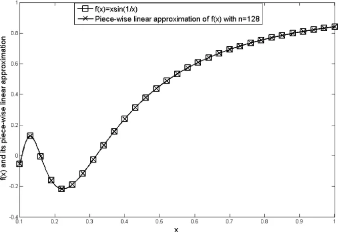
Minimize f(x)=xsin1 x subject to x ∈ [0.1,1].
Which is desirable to be solved with accuracy more thanε=10−3.
Based on our proposed approach we approximate f(x)with a piecewise linear function with global error less than(10−3)2. An appropriate number of parti-tions which is matched with desirable accuracy is obtained asn=128. Figure 1 shows f(x)and its accurate enough piecewise linear approximation.
Figure 1 – Nonlinear function f(x)=xsin1x and it’s piecewise linear approximation.
Nonlinear Global Exact Approximated
function error solution solution
f(x)=xsinx1 5.6527×10⁻⁸ –0.2172336 –0.2174230
Table 5.1 – Numerical results of example 5.1.
Example 5.2. Consider the following minimization problem (see Schuldt [8]):
Minimize f(x,y)=y+10−5(y−x)2 subject to −1≤ x ≤1
0≤ y≤1.
Here it is desirable to solve above problem with accuracy more than ε =10−3. Thus we approximate f(x,y)with a piecewise linear function with global error less than(10−3)3. Table 5.2 compares the solution which is obtained by our proposed approach and exact solution of this problem. It can be shown that proposed approach is effective to solve the problem with desirable accuracy.
Nonlinear Global Exact Approximated
function error solution solution
f(x,y)=y+10−5(y−x)2 2.6615×10⁻¹¹ 0 −5.625×10⁻⁶
Table 5.2 – Numerical results of example 5.2.
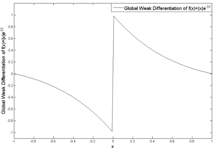
Example 5.3. In this example we consider a nonlinear non-smooth function as follows:
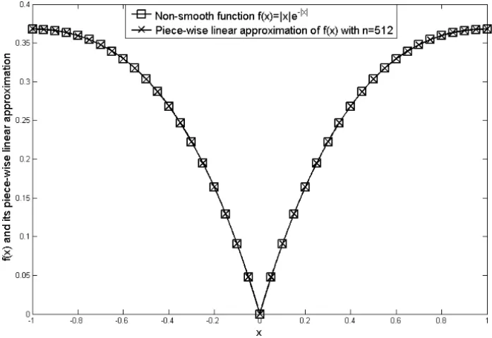
Minimize f(x)= |x|e−|x| subject to x ∈ [−1,1].
It is desirable to solve with accuracy more thanε =10−5
Since objective function is non-smooth function we find the global weak dif-ferentiation of f(x) = |x|e−|x|; x ∈ [−1,1]which is the optimal solution of the following optimization problem:
Minimizep(.)
Z 1
−1
The optimal solution is shown in Figure 2.
Figure 2 – Global Weak Differentiation of nonlinear non-smooth function f(x) =
|x|e−|x|.
Now we find a piecewise linear approximation for non-smooth function f(x) = |x|e−|x| on[−1,1] with the global error less than(10−5)2. Therefore number of partitions should be chosen asn≥512. Figure 3 shows f(x)and its accurate enough piecewise linear approximation withn=512.
Table 5.3 compares approximated and exact solution of last example. Com-parison results show the effectiveness of the proposed approach in the presence of non-smooth functions.
Nonlinear Global Exact Approximated
function error solution solution
f(x)= |x|e−|x| 1.7697×10⁻¹² 0 3.8073×10⁻⁶
Figure 3 – Nonlinear function f(x)= |x|e−|x|and it’s piecewise linear approximation.
6 Conclusion
In this paper we introduce a new approach to solve approximately wide class of constrained nonlinear programming problems. The main advantage of this approach is that we obtained an approximation for the optimum solution of the problem with any desirable accuracy. Also the approach can be extended for problems with non-smooth dynamics by introducing a novel definition of global weak differentiation in the sense ofL1andLpnorms. In this paper we assume
f be a non-smooth function, so it may have a finite or infinite points where the gradient of f does not exist. It is very interesting that we may not know these point (where are located) and also the set of points where the functions are non-smooth may be an infinite set.
REFERENCES
[2] M.S. Bazaraa, H.D. Sherali and C.M. Shetty,Nonlinear Programming: Theory and Algorithms, 2ndEdition, John Wiley and Sons, New York (1993).
[3] Claus Still and Tapio Westerlund, A linear programming-based optimization algorithm for solving nonlinear programming problems, European Journal of Operational Research, Article in press.
[4] A.V. Kamyad and H.H. Mehne, A linear programming approach to the control-lability of time-varying systems, IUST – Int. J. Eng. Sci.,14(4) (2003).
[5] D.G. Luenberger, Linear and Nonlinear Programming, Stanford University, California (1984).
[6] Yehui Peng, Heying Feng and Qiyong Li, A filter-variable-metric method for nonsmooth convex constrained optimization, Journal of Applied Mathematics and Computation,208(2009), 119–128.
[7] W. Rudin, Principles of Mathematical Analysis, Mc Graw-Hill, Inc. (1976).
[8] S.B. Schuldt,A method of multipliers for mathematical programming problems with equality and inequality constraints, Journal of Optimization Theory and Applications,17(1/2) (1975), 155–161.
[9] A.M. Vaziri, A.V. Kamyad, S. Effati and M. Gachpazan, A parametric lin-earization approach for solving nonlinear programming problems, Aligarh Journal Statistics, Article in press.
[10] Ying Zhang, Liansheng Zhang and Yingtao Xu, New filled functions for nonsmooth global optimization, Journal of Applied Mathematical Modelling, 33(2009), 3114–4129.
[11] Yongqing Yang and Jinde Cao, The optimization technique for solving a class of non-differentiable programming based on neural network method, Journal on