ISSN 0101-8205 www.scielo.br/cam
Comparing stochastic optimization methods to solve
the medium-term operation planning problem
RAPHAEL E.C. GONÇALVES∗, ERLON C. FINARDI, EDSON L. DA SILVA and MARCELO L.L. DOS SANTOS
Electical Systems Planning Research Laboratory – LabPlan – EEL – CTC – UFSC Campus Universitário, Trindade, Caixa Postal 88040-900, Florianópolis, SC, Brazil
E-mail: [email protected] / [email protected] / [email protected] / [email protected]
Abstract. The Medium-Term Operation Planning (MTOP) of hydrothermal systems aims to define the generation for each power plant, minimizing the expected operating cost over the
planning horizon. Mathematically, this task can be characterized as a linear, stochastic, large-scale
problem which requires the application of suitable optimization tools. To solve this problem, this
paper proposes to use the Nested Decomposition, frequently used to solve similar problems (as in
Brazilian case), and Progressive Hedging, an alternative method, which has interesting features
that make it promising to address this problem. To make a comparative analysis between these two
methods with respect to the quality of the solution and the computational burden, a benchmark is
established, which is obtained by solving a single Linear Programming problem (the Deterministic
Equivalent Problem). An application considering a hydrothermal system is carried out.
Mathematical subject classification: Primary: 06B10; Secondary: 06D05.
Key words:Hydrothermal Systems, Stochastic Optimization, Medium-Term Operation Plan-ning Problem, Nested Decomposition, Progressive Hedging.
#CAM-174/10. Received: 15/I/10. Accepted: 29/IV/10.
1 Introduction
The Medium-Term Operation Planning (MTOP) problem of hydrothermal sys-tems consists in defining a generation strategy to minimize the production cost over the planning horizon, usually ranging from two months to one year ahead, taking into account constraints associated with the system and the generation plants.
Depending on the regulatory framework, this problem can be solved either by the Independent System Operator (ISO) or by the generation companies that own a mix of hydro and thermal plants, which need to submit bids (price and quantity) to the ISO. Particularly, in Brazil, a similar model is used by the ISO in order to define the dispatch and the spot price1. This model [1] has being improved continuously, aiming to produce a satisfactory response, which opens room for contributions, such as the proposal of this paper.
This problem is particularly complex owing to some characteristics specially related to randomness of water inflows to the reservoirs [2]. Thus, solutions obtained by models that do not recognize this uncertainty produce unsatisfactory results. Additionally, the availability of hydro energy in the future depends on future inflows, which are uncertain, and the reservoirs operation. For instance, assuming that we discharge today as much as possible followed by drought period in the future, it may be necessary to use expensive thermal generation in the future. On the other hand, if the reservoir level is preserved by means of a more intensive use of thermal generation in the present, and wet period occur in the future, spillage may occur (implying a waste of energy). For this reason, the hydro system operation is a problem coupled in time, that is, there is a connection between an operating decision in a given stage and the future consequences of this decision [3].
Besides, the MTOP usually has the following operating characteristics: co-ordination with the long-term problem by means of a future cost function; the water released from one hydro plant affects the production of other plants downstream; the hydro plants are located in different basins, each one with a particular hydrology pattern [4].
1In fact, the spot price is set by the Short Run Marginal Cost obtained as a byproduct of an
In general, some simplifications are introduced into the model with purpose to eliminate some nonlinearities related to the operation cost of thermal power plants and the production function of hydro plants and, so, allowing it to be solved within a reasonable cpu time2. For example, currently in Brazil, the non-linear hydro plant production function is approximated by a piecewise non-linear convex model, which depends on the reservoir volume, discharged outflow and, in some cases, spillage from the reservoir [5].
Like other multistage stochastic optimization problems, the MTOP problem can be classified as a difficult one, given that its size grows exponentially ac-cording to the number of stages and scenarios considered in the problem. Thus, MTOP requires a high computational effort to be solved.
So far, Nested Decomposition (ND) [6] has been used exhaustively to solve similar problems [7, 8] by using algorithms based on a stochastic extension of Benders decomposition [9]. By this approach, the original problem is decom-posed into several subproblems which are easier to solve. The communication between these subproblems is made by the optimality constraints. Then, these constraints are iteratively added to the problem in order to enhance the modeling and, in turn, the solution quality.
Recent advances in the theory of stochastic programming make it possible to develop new methods for solving multistage stochastic programs of remark-able sizes. So, for the multistage stochastic linear programs, the decompo-sition framework based on Augmented Lagrangian (AL) [10] has properties that make it promising for large-scale problems. In this method, some constraints are moved to the objective function generating a simpler but equivalent prob-lem. The resulting subproblems of the decomposition scheme are quadratic, leading to a differentiable problem. When comparing to other methods with the same features, such as the Lagrangian Relaxation (LR) [11], this method has the advantage of obtaining a feasible primal solution.
Progressive Hedging (PH) is an AL based decomposition method that has been broadly applied to similar problems of others fields of knowledge [12, 13]. Due to its solution features it can be an alternative method to solve the MTOP problem.
2In this case, the stochastic characteristic is prioritized in relation to other characteristics of
In this context, the main purpose of this paper is to present a comparative study about the performance of different multistage stochastic optimization methods applied to the MTOP. Therefore, the quality of the solution and the CPU time will be shown. The first method considers the representation of the model through a single Linear Programming (LP) problem, the Deterministic Equiv-alent problem (DE)3 [14]. The main idea of this approach is to establish a benchmark for a comparison with the other methods, which make use of de-composition strategies: the ND and the PH. Both dede-composition algorithms break the MTOP into smaller subproblems and therefore greatly reduce memory requirements. To obtain reliable results, a realistic hydrothermal configuration extracted from the Brazilian hydrothermal power system was used. Addition-ally, sensitivity analyses4were carried out considering different piecewise linear models that describe the hydro plant production function.
The remainder of the paper is organized as follows. In Section 2, a brief de-scription of the multistage stochastic optimization problem features is shown. The list of symbols used in this paper is presented in Section 3. The three problems, related to each solution strategy, are detailed in Section 3. The test problem and the results on solving this problem are shown in Section 4. Finally, conclusions are presented in Section 5.
2 Multistage Stochastic Optimization Problems
The MTOP is a multistage stochastic problem [16] and, therefore, a difficult problem to be solved. In general, computational methods for multistage stoch-astic programming problems can be divided into two main groups [17]. The first group takes advantage of the special features of stochastic problems to improve data structures and solution strategies [18]. The second group uses 3There are two ways of writing DEs: the implicit and the explicit [15]. The difference is the
way in which the constraints (nonanticipativity) are handled. The explicit DE has more variables and more constraints than the implicit DE. There are no practical reasons to solve a stochastic optimization problem by its explicit DE. However, this modeling can be useful once there are several strategies that explore that particular structure. In this paper, the explicit DE will be used by the Progressive Hedging method, while the implicit DE will be used to solve the problems in a single linear programming.
4These studies are important to analyze the trade-off between the solution quality and the
special decomposition methods which exploit the problem structure to split it into manageable pieces and coordinate their solution [19].
As presented in the previous section, in this work three methods are used to solve the MTOP Brazilian problem: (i) the implicit DE: a large-scale LP is given to a commercial package to solve which belongs to the first group of the computational methods [20]; (ii) the ND: a Benders decomposition method; (iii) the PH: an AL-based method.
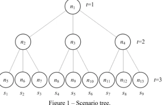
In a multistage stochastic optimization problem, decisions are to be made in stages, and the uncertainties can be modeled by means of a scenario tree that can be generated by sampling techniques [21]. Figure 1 gives an example of a scenario tree for a three stage problem, in which the water inflow to the hydro plants is uncertain. In this structure, each node (filled circle) represents a specific random realization for the water inflow (system state). A branch represents the relationship between two water inflow realizations (state transition). Thus, a scenario consists of a complete path from the node at stage one to a node at stage three. As a consequence, this tree has nine possible scenarios and 13 nodes.
Figure 1 – Scenario tree.
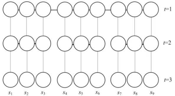
the decisions of nodesn1andn2must be identical for the scenarioss1,s2ands3. The Figure 2 shows a different representation for the same scenario tree as in Figure 1. At this representation, the scenarios are represented by the full lines while the dotted lines link the decisions for different scenarios, representing the nonanticipativity concept.
Figure 2 – Sequences of decisions and nonanticipativity (horizontal dotted lines).
The problem can be modeled in different ways according to the chosen solution method. Therefore, the ND decomposes the problem into stages of decision, in which subproblems correspond to nodes and are linked through the temporary joining constraints, so that the mathematical model corresponds to that shown in Figure 1. Given that we intend to use the PH method, introducing scenario decomposition, the mathematical model must use the nonanticipativity condition to link the subproblems, like in Figure 2.
The mathematical modeling of the problem for each solution method will be detailed on the next sections.
3 Problem formulation
T total stages;
t index of stage, so thatt=1, . . . ,T; E total number of subsystems;
e index of subsystems, so thate=1, . . . ,E; t set of nodes (decisions) on staget;
ω a specific node in the staget, so thatω ǫ t;
S total number of scenarios;
s index of scenario, so that,s=1, . . . ,S; I total number of thermal plants;
i index of thermal plants, so that,i =1, . . . ,I; R total number of hydro plants;
r index of the hydro plants, so that,r =1, . . . ,R; Ŵe set of subsystems linked to the subsysteme;
aω1 immediate ancestor node from nodeω; kω successor node from the nodeω;
Mr set of upstream reservoirs from reservoirr;
m index of upstream reservoirs;
N number of linear constraints used in piecewise linear function of the hydro plant;
n index associated with the piecewise linear function of the hydro plant, so that,n =1, . . . ,N;
J number of linear constraints used in the piecewise future cost function; j index associated with the piecewise future cost function;
Kω set of successor nodes from the nodeω;
Xst set of all scenarios related to scenario s at stagetby the nonanticipativity,
pti power output in thei-th thermal plant [MWh];
de energy deficit in thei-th subsystem [MWh];
α expected value of the operation cost (scalar) from the stageT+1 on; phr power output inr-th hydro plant [MWh];
I ntle power interchange from subsystem l to subsystem e [MWh];
vr final volume of ther-th reservoir[hm3];
Qr discharged outflow in ther-th reservoir[m3/s];
spr spillage in the reservoir of the hydro plant r[m3/s];
v average volume of reservoir[hm3];
pω probability associated to the each nodeω, such that, P ω∈t
pω =1;
cti incremental operation cost of thei-th thermal plant[$/M W h];
cde incremental penalty associated to the energy deficit in thee-th subsystem
[$/MWh];
Le energy demand at subsysteme[MWh];
yr incremental inflow into ther-th reservoir[m3/s];
γrj linear function segment at ther-th reservoir of the system;
π Lagrange multiplier [$/MWh] vector associated with the stream-flow bal-ance constraint;
λ Lagrange multiplier vector associated with the nonanticipativity con-straint;
ρ positive penalty parameter used in the Augmented Lagrangian method; σ zero-spillage adjusting factor of the piecewise production function;
τ minimal total square difference factor of the piecewise production func-tion considering the spillage.
3.1 Deterministic equivalent
more stages and scenarios are considered, it is important to exploit the partic-ular matrix structured and its sparsity as much as possible. In this paper, com-mercial software, CPLEX, was used [23], which uses an advanced optimization algorithm to improve the performance. However, for problems in the real life with the similar structure of the MTOP problem, the usage of CPLEX may not be feasible, given that memory requirements. Indeed, according to the literature [17], multistage stochastic optimization problems, in general, need to be solved by using decomposition techniques, even considering the recent advances in the computing technology.
Therefore, given that we are interested in developing efficient decomposition algorithms to solve MTOP problem in an acceptable time, we make use of the implicit DE approach applied to a small problem5in order to obtain a benchmark solution to other methods.
The problem formulation is presented as follows.
• Objective function
The objective function aims to minimize the system’s operation cost. This cost is composed by thermal fuel costs over the planning horizon plusα future cost, which depends on the reservoir’s volume at the end of this horizon (at the end of stageT). Then, it can be written as:
MinF =
T
X
t=1 X
ω∈t
pω
X
e∈E
X
i∈Ie
ctiptiω+cdedeω
+α. (1)
• The demand supply constraints X
i∈Ie
ptiω+
X
r∈Re
phrω+
X
l∈Ŵe
I ntleω+deω =Leω, e=1,E. (2)
Notice that the hydrothermal system is composed of subsystems that are in-terconnected. In this context, power plants are located in different subsystems defined by the indexesIeandRe, respectively.
Additionally, the demand was considered constant through all stages.
5A problem within a suitable size is build to demonstrate the method’s limitation, considering
• Stream-flow balance constraints vrω−vr aω+Qrω+sprω−
X
m∈Mr
(Qmω+spmω)=yrω, r =1,R. (3)
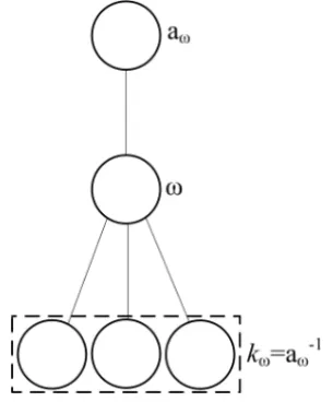
Here, it is important to discuss the successors and the ancestor nodes in the scenario tree. So, observe the Figure 3.
Figure 3 – Structure tree (successor and ancestor node).
Observe that the nodeaω denotes the immediately ancestor node from node
ω. This idea can be expanded for a bigger scenario tree (Fig. 1). Otherwise,aω1 orkωdenotes the successor node from the nodeω.
• Piecewise linear function of the hydro plant
phrω ≤ phnrω vrnω,Qnrω,sprnω
+σrn∂phrω ∂vrω
vrnω,Qnrω,spnrω
vrω−vrnω
+σrn∂phrω ∂Qrω
vnrω,Qrnω,sprnω
Qrω−Qnrω
+τrnsprω, n=1,N,r∈ R.
(4)
i. For all plants, choose N, which is dependent on the precision required. Setsp=0 (ignoring, at the first moment, the spillage).
ii. For each plant,r =1, . . . ,R, setn =0. SetQ0= Qmax.
Let(Q0, v0)be a feasible point, setn =n+1. iii. Whilen< N.
Ifvn=vn−1, calculate ∂phrn
∂Qr v n r,Qr,0
.
Let Qn<Qn−1. If ∂phnr
∂Qr v n r,Qnr,0
> ∂phrn
∂Qr v n
r,Qnr−1,0
.
Return to step 3 and setn=n+1. Else return to step 3.
Else return to step 3 and setn =n+1.
iv. Forn = 0, . . . ,N, find a first order Taylor approximation of the hydro production function.
phrω ≤ phnrω v
n rω,Q
n rω,0
+ ∂phrω ∂vrω
vrnω,Qnrω,0
vrω−vrnω
+∂phrω ∂Qrω
vrnω,Qnrω,0
Qrω−Qrnω
.
v. Based on the first order Taylor approximation, a more realistic approx-imation is obtained by applying a correction scaling factorσ that minim-izes the average square deviation between the real function and approx-imation function.
phrω vrω,Qrω,0
=σphrω vrω,Qrω,0 .
vi. Finally, in order to consider the spillage, forn=0, . . . ,Nuse secant cuts to approximate the hydro production on the dimensionsp, similar to the explained in [5].
phnrω vrω,Qrω,0
=σphrnω vrω,Qrω,0
As a result of this approach, the hyperplanes 4 form a wrap function tangent to the hydro plant production, maintaining, in this way, the problem’s convexity.
• Future cost function
α− X
ω∈T
X
r∈R
γr(j)vrω ≥α (j)
0 , j =1, . . . ,J. (5) This function is given by the longer-term planning model, such as [24] and estimates the expected future cost. It is a piecewise linear function depending on the volume of water in the reservoir at the end of the plan-ning horizon, T. Therefore, it represents the expected future cost from T +1 on. It is worth to notice that these constraints 5 are only included in the subproblems associated with the last stage.
• Power interchange limits between subsystems
−I ntlemaxω ≤ I ntleω ≤ I ntlemaxω , e∈ E, l∈Ŵe. (6)
The variable that describes the power interchange can assume a negative value if the interchange occurs from subsystemeto subsysteml.
• Maximum and minimum volume in the reservoirr vrmin ≤vrω ≤vrmax, vrmin≤vr aω ≤v
max
r ,r ∈ R. (7)
• Limit of the spillage in the reservoirr
sprω ≥0, r ∈ R. (8)
• Limits of the discharged outflow in the reservoirr
0≤ Qrω≤ Qmaxr ,r ∈ R. (9)
• Thermal and hydro production limits
0≤ ptiω ≤ ptimax,i ∈ I,0≤ phrω ≤ phmaxr , r ∈ R. (10)
Then, the MTOP problem can be represented by the Linear Problem model: minF = (1) ,
3.2 Nested decomposition
The ND is a decomposition method based on the Bender’s decomposition prin-ciple. This method solves the first stage problem and deals with the remain-ing stages as other subproblems, solvremain-ing them recursively. In other words, this solves Problem 11 in a recursive manner.
In summary, ND is an iterative process divided into two steps: forward, in which the operative cost for each stage is calculated and passed forward to later stages as input to the right hand side; andbackward, in which the approx-imations costs are fulfilled and passed back from later stages in the form of optimality cuts, also called a Bender’s cut, to the ancestor problem.
In this way, by the application of the single-cut version [8], the Problem 11 is decomposed into subproblems by nodes, which represent a possible water inflow in each stage of the planning horizon. The objective function for the subproblems has the expression:
Fω =
X
e∈E
X
i∈Ie
ctiptiω+cdedeω+Bω
. (12)
The subproblems’s constraints are similar to those presented in the previous section; however, in the Eq. 3, the time coupling constraint, is changed for:
vrω+Qrω+sprω−
X
m∈Mr
Qmatv
ω +spmaωtv
=yrω+vr a(0)ω,r =1,R.
(13)
In this decomposition scheme, the current stage decision depends on the pre-vious stage decision and, therefore,v(0)
r aωdenotes the ancestor node solution. As aforementioned, the cuts created are passed back to the ancestor node subproblem to represent an outer linearization of the recourse function. The expected value of the Lagrange multipliers (dual prices) is used to form the optimality cuts:
Bω−
X
r∈R
X
k∈Kω
pk
pω
where,
Hrω = −
X
r∈R
X
k∈Kω
pk
pω
πr kv(r0ω)+
X
k∈kω
pk
pω
Fk(0), (15)
where vr(0ω) denotes the solution of the previous forward simulation and Fk(0) represents the expected future cost on taking thev(0)
rω decision.
Thus, as the subproblems size is increased iteration after iteration and there are finitely many optimality cuts, the ND method is finitely convergent. Therefore, the initial iterations of this method are very inefficient.
3.3 Progressive hedging
An alternative algorithm to the ND is the PH, which is based on the AL [25]. The fundamental difference between ND and PH is the way that the two algo-rithms address the nonanticipativity constraints. As shown, ND handles these constraints by having a master problem generating proposals to the subproblems further down the tree scenario; proposal are affected by “futures” nodes by opti-mality cuts. In PH a different approach is taken: nonanticipativity constraints are relaxed by expressing the large-scale problem in terms of smaller subproblems that are discouraged from violating the original constraints.
Each scenario subproblem is a deterministic problem and has a separate set of variables. These subproblems are coupled by the nonanticipativity constraints which, as discussed above, stipulate that nodes sharing the same stochastic his-tory up to and including that stage must make the same sequence of decisions.
More precisely, the PH models the nonanticipativity by the average value of these scenarios decisions, such as shown in 16.
ˉ vr st =
Xst
X
x=1
pxvr xt, s =1,St, t =1,T −1. (16)
Applying the AL to the objective function from the DE model, Eq. 1, and considering the nonanticipativity requirement, the subproblems have the fol-lowing structure:
min 3s = ps
T
X
t=1 X
e∈Et
X
i∈Ie
cti(pti st)+cde(dest)
+αs
+ps
"T−1 X
t=1
λr st(vr st− ˉvr st)
#
+ps
" 1 2ρ
T−1 X
t=1
kvr st− ˉvr stk2
#
,
s.t.: X
i∈Ie
pti st+
X
r∈Re
phr st+
X
l∈e
I ntlest +dest =Let,
vr st −vr s,t−1+Qr st+spr st −
X
m∈Mr
Qms,t−tv+spms,t−tv
=yr st,
phr st ≤ phnr st(.)+
∂phr st
∂vr st
(.) vr st−vr stn
+ ∂phr st ∂Qr st
(.) Qr st −Qnr st
+∂phr st ∂spr st
(.) spr st−spr stn ,
αs −
X
r∈R
γr(j)vr sT ≥α
(j)
0 , j=1, . . . ,J, −I ntlestmax≤ I ntlest ≤ I ntlestmax,
vrmin≤vr st ≤vrmax, 0≤ phr st ≤ phrmax,
0≤ Qr st ≤ Qmaxr , 0≤ pti st ≤ ptimax, spr st ≥0,
e∈ E, l∈Ŵe, r ∈ R,
s =1, . . . ,St, t =1, . . . ,T, n =1, . . . ,N.
(17)
Notice that in the AL function there exists an additional parameter,v, for eachˉ iteration, which is used to uncouple these subproblems for all scenarios [26].
The solution algorithm of the PH consists in an iterative process which solves the subproblems 17 and the dual problem 18:
max ψ (λ)=
S
P
s=1
ψs(λs),
s.t.: λ ∈ Rm.
Since the dual problem 18 is differentiable, it can be solved by applying of the gradient method:
λi terr,s,t+1=λi terr,s,t+ρ vr,s,t− ˉvr,s,t
. (19)
This method has two parameter sets that are iteratively updated: the additional parametervˉ and the Lagrange multipliers. Besides, the gradient method only uses information from the last iteration. Owing to these features, the PH is also sensitive to the use of warm start [27].
This class of methods has some advantages when compared to other meth-ods: the primal solution feasibility is guaranteed and it has a weak link between scenarios. The weak link means that in case of computational parallelization, only little information needs to be shared by the processors. The only commu-nication requirement is a share of scenario solutions to enforce nonanticipativity constraints. Thus, this algorithm is suitable for paralleling processing.
4 Computational results
To observe the efficiency of the methods, a performance analysis of each method facing test systems with different complexities are shown. For that, a real hy-drothermal system is modeled into two different LP problems, differing from each other by the precision of the hydro production model6. In the first case, the hydro plant production is modeled by a piecewise linear function only depending on the discharge outflow, resulting in three linear functions. In the second case, the piecewise linear function is more accurate and it depends on the reservoir storage, discharged outflow and spillage.
In this paper, with the purpose of presenting a coherent analysis of the methods, the computational time was used as the stop criterion.
Before showing the study cases, a brief description of the hydrothermal system is presented.
6It is important to state that the models of hydro production function are not the focus of
4.1 Test problem
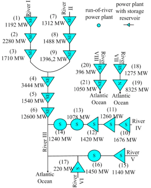
The hydrothermal system is based on the Brazilian system and made up of 21 hydro and 20 thermal plants. The total installed capacity is about 57 GW and the demand is about 66% of this value.
The hydro plants are physically connected in cascades, as depicted in ure 4. This hydro configuration has approximately 47 GW installed. In the Fig-ure 4, the indexes SE, S, NE and N represent the subsystems Southeast, South, Northeast and North, respectively, in which the Brazilian system is subdivided.
Figure 4 – Test system of hydro plants.
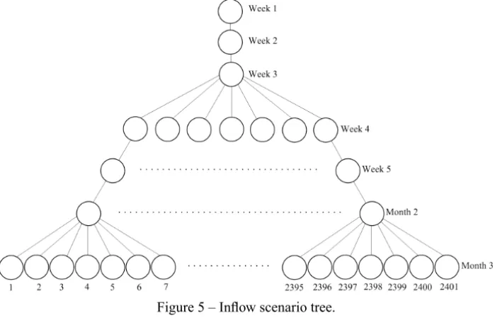
The stochastic model has a study period made up of five weeks plus two months, as depicted in Figure 5, similar to the Brazilian MTOP. The first three stages (three weeks) are modeled as deterministic and the remaining stages as stochastic, each one with seven possible realizations. This scenario model was generated by the periodic autoregressive (PAR) model [30] that is made available by the ISO.
Figure 5 – Inflow scenario tree.
All models of LP (DE and ND) as well as the quadratic programming prob-lems resulting from the PH were solved by the commercial software ILOG CPLEX 7.1. Tests were performed on an Intel Core2 Duo 2.33GHz with 2GB of RAM.
4.2 Case I
In this case, the hydro plant production is represented by a piecewise linear function with three constraints. In addition, this function depends only on the discharged outflow of the hydro plant. This is a simplified model that does not consider the impact of the water head on the production function.
was fixed in five, once the cpu time requested is significantly higher when com-pared with ND.
Thus, the comparative study is presented in the Table 1. It is important to say that in this case the DE problem has 441,492 variables and 348,323 constraints (101,582 are equality constraints and 246,741 are inequality constraints).
Computation Objective Methods Iteration
time (h) function Deviation ($ millions)
Deterministic Equivalent — 1.277 96.80 —
Nested Decomposition 21 1.517 96.86 0.070%
Progressive Hedging 5 3.254 96.42 0.391%
Table 1 – Methods comparison – Case I.
The deviations shown in refer to the solution deviation of each methodology (objective function) with respect to the DE solution, which is the exact solution. Notice that the DE method presents the best cpu performance when compared with other methods. Additionally, it can also be observed that ND has reached a better solution faster than PH.
4.3 Case II
The aim of this case is to demonstrate that problem’s size increases, the use of DE can be infeasible and, at the same time, to analyze the performance of the other methods against this benchmark.
In contrast to Case I, the hydro plant production is modeled by a piecewise linear function depending on the reservoir storage, the discharged outflow and the spillage. Moreover, this function has five linear constraints. In others words, five points are used to construct the piecewise linear approximation.
In a different way to the Case I, due to preliminary tests, the value of the PH’s penalty parameterρis 0.1. For both decomposition methods, the compu-tational time was considered as the stop criterion and both should be similar for propitiating a suitable comparison. Additionally, the PH uses the solution of the expected value problem [19] to set additional parameter7; therefore this approach works as a warm start.
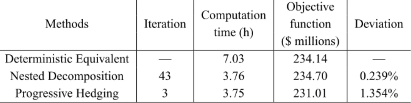
The comparative analysis between each algorithm is shown in Table 2. The DE problem has 441,492 variables and 492,282 constraints, with 390,700 in-equality constraints. Each ND subproblem (node subproblem) in its first itera-tion has 113 variables and 126 constraints, which 100 are inequality constraints, except in the last stage where it has 114 variables and 726 constraints due to the expected future cost function, summing up 700 inequality constraints. It is worth pointing out that in the ND method, the number of constraints increases at each iteration. On the other hand, each quadratic programming subproblem resulting from the PH decomposition (scenario subproblem) has a fixed set of 792 variables and 1482 constraints, which 1300 are inequality constraints.
Computation Objective Methods Iteration
time (h) function Deviation ($ millions)
Deterministic Equivalent — 7.03 234.14 —
Nested Decomposition 43 3.76 234.70 0.239%
Progressive Hedging 3 3.75 231.01 1.354%
Table 2 – Methods comparison – Case II.
First of all, notice that the production cost resulting from this case is approx-imately two times greater than the obtained in the previous case. This occurs because in Case II we used a more realistic model regarding the volume vari-ation8 and spillage9. It is important to model this characteristic because the volume variation in some reservoirs is significant and the spillage is quite common in some plants.
Also, according to Table 2, observe that ND and PH have obtained satisfac-tory results in a small cpu time in comparison to the DE approach10, although 8In the Case I, although it has been calculated three linear functions, the reservoir volume is
considered constant in each of them.
9The gross head of a reservoir is given by the difference between the forebay and tailrace
levels. The net head is defined by the gross head minus the penstock head losses. The forebay level depends on the reservoir volume while the tailrace level is dependent on the total discharged outflow and, in some cases, is also dependent on the spillage. So, considering that a reasonable precision is desired, the modeling of the net head is a critical aspect of problem. For more detail, see [5].
the PH did not already find a feasible solution11.
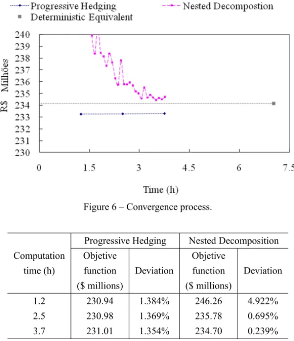
Figure 6 illustrates the convergence process of Case II. Observe that if both algorithms were limited to almost one hour of processing, the smallest deviation would be given by the PH. On the other hand, if the time limit was close to two hours and thirty minutes, the PH presents a deviation slightly bigger than the ND. Finally, if the stop criterion was extended to close to four hours, the ND presents the best solution. The Table 3 illustrates these comments.
Figure 6 – Convergence process.
Progressive Hedging Nested Decomposition
Computation Objetive Objetive
time (h) function Deviation function Deviation ($ millions) ($ millions)
1.2 230.94 1.384% 246.26 4.922%
2.5 230.98 1.369% 235.78 0.695%
3.7 231.01 1.354% 234.70 0.239%
Table 3 – Methods evolution.
In agreement with Table 2, the number of iterations of ND is bigger than PH. 11Given that ND converged at the cpu time of 3.7 hours, we used this reference as the stop
The ND subproblems are linear and refer to nodes while the PH subproblems are quadratic and refer to scenarios. Therefore, each iteration in the PH method requires more time than the ND method.
These results show that the precision of the mathematical modeling can inter-fere with the method’s performance. In other words, the increase of the problem size (which in this paper depends on the hydro plant’s production accuracy) af-fects the convergence for each method. Additionally, operation cost in Case II is higher than in Case I (as expected), given that a more accurate modeling is used for the hydro plant production. As a consequence, in Case II a larger computational effort is required.
Also, although the ND and PH methods require more computational time than the Case I, now they require less time than the DE to reach lower devi-ations. This proves that as the size of the problem increases the DE requires more computational cpu time, making its application prohibitive for large systems12. We can also observe that ND is more sensitive than PH with respect to the problem’s size; this may be an indicative that for bigger problems PH will work better than ND.
5 Conclusions
The objective of the hydrothermal systems MTOP is to calculate an operation strategy for the purpose of minimizing the operation cost over a time horizon. Owing to the uncertainties associated with the inflows scenarios, this problem is quite complex and addressed as a multistage stochastic programming problem. In this paper we compare three solution methods: (a) Deterministic Equivalent, (b) Nested Decomposition, and (c) Progressive Hedging.
Although the Deterministic Equivalent can offer the exact solution, its ap-plication in a large-scale problem may be infeasible due to the huge memory requirements and high computational burden. Thus, alternative approaches like Nested Decomposition and Progressive Hedging methods constitute interesting paths to be investigated.
12It is important to say that limitation in memory occurs when the size of the problem increases.
Additionally, it is important to emphasize that the accurate representation of the hydro plant production inserts an additional complexity into this particular problem but, as benefit, it improves the quality solution. Certainly the results obtained in the Case I cannot implemented in real life. This fact can be ob-served when it is compared the computational time and the operation cost of the cases I and II.
Studies presented demonstrated that the Equivalent Deterministic is not useful to solve huge problems and that the Progressive Hedging is competitive when compared to the Nested Decomposition. Moreover, the Progressive Hedging is more stable than the Nested Decomposition, allowing for good so-lutions with less computational time and for bigger problems PH may respond better than ND.
REFERENCES
[1] M.E.P. Maceira, L.A. Terry, F.S. Costa, J.M. Damázio and A.C.G. Melo, Chain of Optimization Models for Setting the Energy Dispatch and Spot Price in the
Brazilian Syste, presented in: 14th PSCC Proceedings, Seville, Spain (2002).
[2] L.F. Escudero, WARSYP: a robust modeling approach for water resources system
planning under uncertainty. Annals of Operations Research,95(2000), 313–339.
[3] E.C. Finardi and E.L. da Silva, Solving the Hydro Unit Commitment Problem via
Dual Decomposition and Sequential Quadratic Programming. IEEE Transactions
on Power Systems,21(2) (2006), 835–844.
[4] M.V.F. Pereira and L.M.V.G. Pinto, Application of Decomposition Techniques to
the Mid- and Short-Term Scheduling of Hydrothermal Systems. IEEE Transactions
on Power Systems,PAS-102(11) (1983), 3611–3618.
[5] A.S.L. Diniz and M.E.P. Marceira, A Four-Dimensional Model of Hydro Gen-eration for Short-Term Hydrothermal Dispatch Problem Considering Head and
Spillage Effects. IEEE transactions on power systems,23(3) (2008), 1298–1308.
[6] M.A.H. Dempster and R.T. Thompson, Parallelization and aggregation of nested
Benders decomposition. Annals of Operations Research,81(1998), 163–187.
[7] D.P. Morton, An enhanced decomposition algorithm for multistage stochastic
hydroelectric scheduling. Annals of Operations Research,64(1996), 211–235.
[8] M.V.F. Pereira and L.M.V.G. Pinto, Stochastic Optimization of a Multireservoir
Hydroelectric System: A Decomposition Approach. Water Resources Research,
[9] J.F. Benders,Partitioning Procedures for Solving Mixed Variables Programming
Problems. Numerische Mathematik,4(1962), 238–525.
[10] A. Ruszczynski, Augmented Lagrangian Decomposition for Sparse Convex
Optimization. Annals of Operations Research (1992).
[11] R. Fuentes-Loyola, V.H. Quintana and M. Madrigal, A Performance Comparison of Primal-Dual Interior Point Method Vs Lagrangian Relaxation to Solve the
Medium Term Hydro-Thermal Coordination Problem. presented at IEEE Power
Engineering Society Summer, Seattle,4(2000), 2255–2260.
[12] R.T. Rockafellar and R.J.B. Wets, Scenarios and Policy Aggregation in
Opti-mization under Uncertainty. Mathematical of Operations Research, 16(1991),
119–147.
[13] J.P. Watson, D.L. Woodruff and D.R. Strip,Progressive Hedging Innovations for
a Stochastic Spare Parts Support Enterprise Problem. Journal Article – Naval
research Logistics (2007).
[14] K.K. Lau, Multistage quadratic Stochastic Programming. Ph.D. dissertation, Dept. Mathematics, Univ. New South Wales (1999).
[15] R. Fourer and L. Lopes, A Management System for Decomposition in Stochastic
Programming. Annals of Operations Research,142(1) (2006), 99–118.
[16] G. Infanger, Planning under uncertainty: Solving Large-Scale Stochastic Linear
Programs. Ed. Boyd & Fraser Publishing Company (1994).
[17] C. Rosa and A. Ruszczynki,On Augmented Lagrangian Decomposition Methods
for Multistage Stochastic Programs. Annals of Operations Research (1996).
[18] V.R. Sherkat, K. Moslehi, E.O. Sanchez Lo and J.G. Diaz,Modelar and Flexible
Software for Medium and Short-Thermal Scheduling. IEEE Transactions on Power
Apparatus and Systems,3(2) (1988), 1390–1396.
[19] J.R. Birge and F. Louveaux, Introduction to Stochastic Programming. 1st ed., New York: Springer (1997).
[20] R. Fuentes-Loyola and V.H. Quintana, Medium-Term Hydrothermal
Coordi-nation by Semidefinite Programming. IEEE Transactions on Power Systems,
18(4) (2003), 1515–1522.
[21] J. Dupaèová, G. Consigli and S.W. Wallace, Scenarios for Multistage Stochastic
Programs. Annals of Operations Research,100(2000), 25–53.
[22] A.J. Berger, J. Mulvey and A. Ruszczynski, An Extension of the DQA
algo-rithm to Convex Stochastic Programs. SIAM Journal of Optimization,4(1994),
[23] ILOG,ILOG CPLEX 7.1. User’s Manual (2001).
[24] E.L. da Silva and E.C. Finardi, Parallel Processing Applied to the Planning of
Hydrothermal Systems. IEEE Transactions on Parallel and Distributed Systems,
14(8) (2003), 721–729.
[25] D.P. Bertsekas, Nonlinear Programming. 2nd ed., Belmont: Athena Scientific (1999).
[26] A. Ruszczynki, Decomposition methods in stochastic programming. Mathem-atical Programming,79(1997), 333–353.
[27] M.L.L dos Santos, E.L. da Silva, E.C. Finardi and R.E.C. Gonçalves, Solving the Short Term Operating Planning Problem of Hydrothermal Systems by Using the
Progressive Hedging Method, presented at 16th PSCC, Glasgow, Scotland (2008).
[28] J. García-González and G.A Castro, Short-term hydro scheduling with cascaded
and head-dependent reservoirs based on mixed-integer linear programming. In:
Power Tech Proceeding, 2001 IEEE Porto,3(2001).
[29] G.W Chang, M. Aganagic, J.G. Waight, J. Medina, T. Burton, S. Reeves and M. Christoforidis, Experiences with mixed integer linear programming based
ap-proaches on short-term hydro scheduling. IEEE Transactions on Power Systems,
6(4) (2001), 743–749.
[30] M.E.P. Maceira and J.M. Damázio, The use of PAR(p) model in the Stochastic Dual Dynamic Programming Optimization Scheme used in the operation
plan-ning of the Brazilian Hydropower System. In: 8th International Conference on