ISSN 0101-8205 www.scielo.br/cam
A semi-analytical computation of the Kelvin kernel
for potential flows with a free surface
JORGE D’ELÍA∗, LAURA BATTAGLIA∗ and MARIO STORTI∗ Centro Internacional de Métodos Computacionales en Ingeniería (CIMEC)
Instituto de Desarrollo Tecnológico para la Industria Química (INTEC) Universidad Nacional del Litoral – CONICET
Güemes 3450, 3000-Santa Fe, Argentina
E-mails: [email protected] / [email protected] / [email protected] / web page: http://www.cimec.org.ar
Abstract. A semi-analytical computation of the three dimensional Green function for seakeep-ing flow problems is proposed. A potential flow model is assumed with an harmonic dependence on time and a linearized free surface boundary condition. The multiplicative Green function is expressed as the product of a time part and a spatial one. The spatial part is known as the Kelvin kernel, which is the sum of two Rankine sources and a wave-like kernel, being the last one written using the Haskind-Havelock representation. Numerical efficiency is improved by an analytical integration of the two Rankine kernels and the use of a singularity subtractive technique for the Haskind-Havelock integral, where a globally adaptive quadrature is performed for the regular part and an analytic integration is used for the singular one. The proposed computation is em-ployed in a low order panel method with flat triangular elements. As a numerical example, an oscillating floating unit hemisphere in heave and surge modes is considered, where analytical and semi-analytical solutions are taken as a reference.
Mathematical subject classification: Primary: 33F05; Secondary: 65N38.
Key words: green function, boundary integral equation, three dimensional potential flow, free surface, computational techniques.
#CAM-155/09. Received: 25/XI/09. Accepted: 08/II/10.
1 Introduction
In seakeeping flow problems for ship hydrodynamics, a rigid body placed on the free surface of an incompressible inviscid fluid can oscillate in any of the six degrees of freedom around its mean position due to a passing front wave [1]. The standard potential flow theory assumes that the motion is relatively small and harmonic in time [2, 3].
The classical analysis with a linearized free surface boundary condition splits the problem into seven parts. First, six radiative modal potentials8k(x,t)have
to be determined, fork = 1,2, . . .6, where the rigid body performs imposed small harmonic oscillations in each degree of freedom, wherexis the position vector andtis the time. Next, a diffraction potential87(x,t), due to a passing harmonic monochromatic wave of small amplitude, has to be found. These modal velocity potentials8k(x,y,z,t), fork =1,2, . . . ,7, are found by solving seven
boundary integral equations, where the left hand sides have the same integral operator and only the independent terms are specific for each mode, e.g. see [4]. As it is well known, boundary element methods, or panel methods [5], are a natural choice for obtaining numerical solutions of boundary integral equations [6] through collocation or Galerkin techniques [7], as well as they are closely related to the Green function theory [8].
The Green functionG(x,ˆ t)for seakeeping is expressed as the product of a time factorT(t)and a spatialG(x)one. Since the incident front wave is assumed to be monochromatic in time, with absolute circular frequencyω, then, the time factor takes the simple formT(t)=eiωt, and all computations can be performed in the
frequency domain. The spatial part of the Green function G(x)is also known as the Kelvin kernel which, in turn, is decomposed into the sum of two Rankine kernels and a wave kernel. Both Kelvin and Rankine kernels are widely used in numerical ship hydrodynamics, although neither of them satisfy the slip boundary condition over the wetted hull surface and, consequently, such condition must be enforced for a numerical computation.
problems with non-linear boundary conditions [9, 10].
On the other hand, the use of the Kelvin kernel avoids the discretization of the free surface, and the outgoing radiation boundary condition is automatically satisfied. However, it involves several rather elaborated mathematical expres-sions and tends to be ill-conditioned for field points nearby the axisymmetric axis of the local cylindrical frame at each panel, which is a serious numerical drawback, particularly in hull meshes with a relatively high number of panels.
Similar approaches have also been considered by Telste-Noblesse [11] and by Ponisy et al. [12]. For instance, in [11] eight expressions were proposed in complementary regions of the spatial coordinate d, between the field point and the mirror image of the source point in the mean sea plane, given by: two asymptotic expansions for large values of the distanced, two ascending series for small values ofd, two Taylor series around the vertical axis, and two expres-sions for intermediate values ofd.
In this work, a computation of the Kelvin kernel is proposed through a singu-larity substraction technique, where the boundary integral is split into the sum of a regular term and a singular one. For the regular term, a globally adaptive numerical quadrature is employed, while for the singular one an analytic inte-gration is performed. The proposed computation is performed with a low order panel method where only the wetted surface of the body in hydrostatic state is discretized with flat triangles. As a numerical example, the oscillating floating hemisphere of unit radius in heave and surge modes is considered, for which there are analytical and semi-analytical solutions.
2 Seakeeping flow problem
2.1 Differential formulation
A Cartesian (x,y,z) coordinate system is chosen, where the z = 0 plane matches the still water plane and the z-axis is positive upwards. The com-plexeiωtdependency of the timetis implicitly assumed, whereωis the circular
frequency of the periodic motion.
linearized governing equation [13]
1φk =0 forz<0;
∂zφk = Kφk atz =0;
φk =O(|x|−1) for|x| → ∞;
(1)
where1 = ∂x x +∂yy +∂zz is the three-dimensional Laplacian operator, φk is
thek-modal radiation potential, and K =ω2/g is the wave-number for gravity waves in deep water.
2.2 Boundary integral equation
A boundary integral equation for solving Eq. (1) is given by [2]
1
2φk(x)+ 1 4π
Z
S
dSξ G,n(x,ξ)φk(ξ)= Qk(x); (2)
forx ∈ S, wherexandξ are the field and source points, respectively, and S is the boundary of the flow domain. The independent term is
Qk(x)=
1 4π
Z
S
dSξ G(x,ξ)σk(ξ); (3)
whileφk(x), fork = 1, . . . ,6, is the k-radiation velocity potential, andσk are
known fluxes. A standard panel method imposes the integral boundary equa-tion (2) by means of a collocaequa-tion technique at the panel centroids, obtaining a complex valued linear systemAφk = Cσk =bk, whereφk is thek-velocity
potential vector, andσk is thek-flux vector corresponding to thek-mode. The
dipolar matrix, which is non-symmetric and regular, is given by
Ai j =
1 4π
Z
S
dSξ G,n(x,ξ); (4)
and the monopolar one, symmetric, is
Ci j =
1 4π
Z
S
dSξ G(x,ξ) . (5)
2.3 Kelvin and Rankine kernels in the spatial Green function
The spatial Green functionG(x,ξ) in Eq. (5) that satisfies Eq. (1), is known as the Kelvin kernel, which gives the interaction between the field pointx = (x,y,z) and the source point ξ = (ξ, η, ζ ) [14]. The physical meaning of the Green function is given by the real part Re{Geiωt
}, which is the disturbed velocity potential measured at the field pointx, at timet, caused by a pulsating sourceξ of circular frequencyωand unit intensity [1]. It should be noted that the outgoing radiation and free surface boundary conditions are automatically satisfied by the Kelvin kernel.
Due to the local axisymmetry around the source pointξ, it is convenient to
introduce the non-dimensional cylindrical coordinates
X =K{(x−ξ )2+(y−η)2}1/2;
Y =K|z+ζ| ; (6)
whereXis the radial coordinate andY the vertical one. Then, the Kelvin kernel for seakeeping is written as
G =r−1+s−1+ ˜G; (7) where
r,s = {(x−ξ )2+(y−η)2+(z∓ζ )2}1/2; (8) are the Euclidean distances between the field pointx and the source point ξ,
and between the field pointxand the image pointξ′=(ξ, η,−ζ ), respectively. In Eq. (7) the first two terms,r−1ands−1, are the Rankine kernels, while the
˜
G term inherits the spatial wave properties of the Kelvin kernel and, then, it is termed the “wave-kernel”.
2.4 Haskind-Havelock representation of the wave-kernel
The wave kernelG˜ involves several transcendental functions and, consequently,
The Haskind-Havelock representation for the wave part of the Kelvin kernel is written as [14]
˜
G(X,Y)= −πK e−Y[H0(X)+Y0(X)+P0(X,Y)+2i J0(X)] ; (9)
whereH0(X)is the Struve function of zero order,J0(X)andY0(X)are the zero order Bessel functions of first and second kind, respectively [15], and P0(X,Y) is the Haskind-Havelock integral [14]
P0(X,Y)= 2 π
Z Y
0
dα e
α √
α2+X2 . (10) The asymptotic behavior of the Kelvin kernel given by Eq. (7), at very low and very high frequencies, will be dealt with in Secs. 4.2 and 4.3.
3 Evaluation of the Kelvin kernel
3.1 Rankine kernels
The Rankine kernelsr−1ands−1can be evaluated in several ways. One possibil-ity is a numerical integration, which has the advantage that high order distribu-tions can be considered without further complicadistribu-tions. However, the numerical integration is rather sensitive to the mesh quality and, moreover, the diagonal terms would deserve a special treatment. Another alternative is an analytic in-tegration, where the surface integral over each panel is replaced by its closed contour integration and a side local reference frame is used for each side contri-bution [16, 17, 18].
3.2 Normal derivative of the Haskind-Havelock kernel
The normal derivative of the Haskind-Havelock kernel is found from G˜,n =
(∇ξG,˜ nξ), where n = (nξ,nη,nζ) is the unit normal of dSξ and ∇ξG˜ =
(G˜,ξ,G˜,η,G˜,ζ) is the gradient ofG, both evaluated on the source point ξ =
(ξ, η, ζ ). By the chain rule in Eqs. (6) and (9)
˜
G,ξ = ˜G,XX,ξ; ˜
G,η= ˜G,XX,η; ˜
G,ζ = ˜G,YY,ζ;
where
X,ξ = −K2(x−ξ )/X;
X,η= −K2(y−η)/X;
Y,ζ =Ksign(z+ζ ) .
(12)
Note that the gradients of the wave-kernel of the Green function, evaluated on the field pointx=(x,y,z)and the source pointξ =(ξ, η, ζ )are linked as
(G˜,ξ,G˜,η,G˜,ζ)=(− ˜G,x,− ˜G,y,G˜,z) . (13)
The complex kernel is
˜
G = ˜G′+iG˜′′; (14)
where the real part, Re{..} ≡ (..)′, and the imaginary one, Im{..} ≡ (..)′′, are given by
˜
G′ = −λ(H0+Y0+P0);
˜
G′′ = −λ(2J0);
λ=πK e−Y .
(15)
The partial derivatives ofG˜′are
˜
G′,X = −λ(H0,X+Y0,X +P0,X); ˜
G′,Y = − ˜G′−λP0,Y ;
(16)
and the corresponding ones ofG˜′′, with J0˙ =dJ0(X)/dX,
˜
G′′,X = −λJ0˙ ;
˜
G′′,Y = − ˜G′. (17)
3.3 Ill-conditioning of the Haskind-Havelock kernel
The Haskind-Havelock finite integral is given by
P0= 2 π
Z Y
0
dα e
α
(α2+X2)1/2 ; (18)
and its partial derivatives are
P0,X = −
2 πX
Z Y
0
dα e
α
P0,Y =
2 πe
Y(Y2
+X2)−1/2. (20)
The Haskind-Havelock finite integral P0 evaluated at t = 0 tends to be ill-conditioned when X ≪ 1, that is, for field points near the axisymmetric axis. This is a serious numerical drawback, in particular in hull meshes with a high number of panels. For overcoming this disadvantage, a singularity subtraction technique is proposed, where the integral is split into the sum of a regular term and a singular one. For the regular term, a globally adaptive numerical quadrature is employed, while for the singular one an analytic integration is performed. On the other hand, a direct computation of the Struve functions H0 and J0can be performed through their definitions and asymptotic expansions.
4 Semi-analytical computation of the Haskind-Havelock kernel
4.1 Singularity subtraction technique
The Haskind-Havelock integral given by Eq. (18) is split into the sum of a regular term and a singular one. For the regular term, a globally adaptive numerical integration can be used, while for the singular one an analytic in-tegration is performed. Thus, Eq. (18) is rewritten as
P0= 2
π(Pˆ0+ ˜P0); (21) where
ˆ
P0=
Z Y
0
dα e
α −1
(α2+X2)1/2 ; (22) is a regular integral which can be evaluated accurately by a globally adaptive integration, for example, the qag routines of the Netlib Repository
(http://www.netlib.org). The remaining integral
˜
P0=
Z Y
0
dα 1
(α2+X2)1/2 ; (23)
contains a logarithmic singularity when X = 0, and it is ill-conditioned when X → 0. Then, it is evaluated in a closed form by performing the following variable changes
α =Xsinh(θ ); dα =Xcosh(θ )dθ ;
(α2+X2)1/2= Xcosh(θ );
for which
α1=0 → θ1=0;
α2=Y → θ2=sinh−1(Y/X); (25) then
˜
P0=
Z θ2 0
dθ =sinh−1(Y/X) . (26)
The partialX-derivative of Eq. (21) is similarly decoupled as
P0,X =
2
π(P0ˆ ,X + ˜P0,X); (27) where
ˆ
P0,X = −X Z Y
0 dαe
α−(1+α+α2/2)
(α2+X2)3/2 ; (28) is a regular integral, whereas
˜
P0,X = −X Z Y
0
dα1+α+α 2/2
(α2+X2)3/2 ; (29)
is the integral that contains the singularity and it is computed in closed form. The variable changeα =Xsinhθ is introduced again and
˜
P0,X = Z θ2
0
dθ −1−Xsinhθ −X
2/2 sinh2θ
Xcosh2θ . (30)
As cosh2θ −sinh2θ =1, then
˜
P0,X =
X2/2−1
X A−
1 XB−
X
2C . (31)
The Aterm is given by
A=
Z θ2 0
dθ
cosh2θ ; (32)
with the variable change
v=eθ → dθ =dv/v;
cosh2θ =(v+v−1)2/4. (33)
Replacing
A=
Z θ2 0
4vdv (v2+1)2 =
−2 v2+1
and then
A=1− e
−θ2
coshθ2 . (35)
Next, theBterm is given by
B =
Z θ2 0
Xsinhθdθ
cosh2θ ; (36)
introducing the variable changes
u =coshθ ; du =Xsinhθdθ ;
α =Xsinhθ ; u =(X2+α2)1/2; (37) for which
α1=0 → u1=X ;
α2=Y → u2=(X2+Y2)1/2; (38) it results
B= X−X2(X2+Y2)−1/2. (39) Finally, the trivialCterm is
C =θ2=sinh−1(Y/X) . (40) However, when the field pointx =(x,y,z)is on the axisymmetric axis of the source pointξ =(ξ, η, ζ ), thenX =0 and these expressions are not applicable. In such case, the asymptotic representation [13]
˜
G(X,Y)=2
∞ X
k=0
Wk(X,Y)−2πi J0(X); (41)
can be used whenX ≪1, where
Wk(X,Y)=
(−X2/4)k
(k!)2 bk ; (42) with
bk =
2k X
j=1
(j−1)! Yj −e
−YEi(Y) for X
where Ei(Y)is the exponential integral [15]. Then
˜
G=2W0+2
∞ X
k=1
Wk(X,Y)−2πi J0(X); (44)
that is
˜
G= −2e−YEi(Y)+2
∞ X
k=1
Wk(X,Y)−2πi J0(X); (45)
which is valid for X ≪ 1. As Wk(X,Y)and its derivatives tend uniformly to
zero in a small neighborhood ofX =0, then, Eq. (45) can be written at X =0 as
˜
G= −2[e−YEi(Y)+πi J0(X)];
˜
G,X =2πi J1(X); ˜
G,Y =2e−Y[Ei(Y)+e−Y/Y].
(46)
In summary, seven expressions are employed for the complementary regions of the coordinatesX andY given by: (i) two regular integrals given by Eqs. (22) and (28), (ii) two analytic integrals given by Eqs. (26) and (31), for X ≫ 1, with the constants A, BandCgiven by Eqs. (35), (39) and (40), and (iii) three approximate expressions given by Eq. (46) forX ≪1.
-0.008 -0.004 0 0.004
-40 -20 0 20 40
x
Im [ G_{,z} = KG ] -0.004
0 0.004 0.008
-40 -20 0 20 40
x Re [ G_{,z} = K G ]
Figure 1 – Real (left) and imaginary (right) parts of the free surface boundary condition
G,z = K G atz = 0, due to a square panel of length L = 0.1, submerged at depth
H=1 and pulsating at frequencyω.
4.2 Kelvin kernel at very low frequencies or near the vertical axis
and, consequently, the square bracket results bounded[. . .] < D, with D as a constant independent of K. Then, when the field pointx =(x,y,z)does not match the source oneξ =(ξ, η, ζ ), the Kelvin kernel has the asymptotic form
G→r−1+s−1forK →0 (low frequencies) orX →0 (near the vertical axis).
4.3 Kelvin kernel at very high frequencies or points far away
For very high frequenciesK ≫1 or points far away from the origin, it is verified thatX ≫1 and, then, the following expansion can be used [1]
Z Y
0
dα e
α−Y √
α2+X2 ≈ 1
√
Y2+X2 +O(s
−3)
; (47)
which is valid for X ≫1. From this,
P0≈ 2 π
eY
√
Y2+X2 = 2 π
eY
K s . (48)
Moreover (see Abramowitz-Stegun [15])
Jn ≈ p
2/(πX)cos(X−nπ/2−π/4);
Yn≈ p
2/(πX)sin(X −nπ/2−π/4);
H0≈Y0(X)+O(1/X);
(49)
thereforeJn,Yn,H0∼ O(X−1/2)and ˜
G≈ −2πK e−Y(Y0+i J0)−2s−1 ; for X ≫1. (50) Thus, for very high frequenciesK ≫1 or points far away from the origin, it is verified that, forX ≫1, the wave kernel has the asymptotic formG˜ → −2s−1. Then, the Kelvin one has the asymptotic formG →r−1−s−1forK ≫1 (high frequencies) orX ≫1 (far away).
4.4 Direct computation of the special functions
The Struve differential equation is (see chap. 9, Abramowitz-Stegun [15])
z2d 2
w dz2 +z
dw dz +(z
2
−ν2)= 4(z/2)
ν+1
√π Ŵ(ν
wherez = x +i y is the complex variable andŴ is the factorial function. Its general solution is
w=a Jν(z)+bYν(z)+Hν(z); (52)
whereJν andYν are the Bessel functions, of first and second kind, respectively,
Hν is the Struve one, all these of integer orderν, anda,bare constants. A direct
computation involves ascending and descending series. The ascending series for the Bessel function of first class Jn(X)and ordern =0,1 are
J0(X)=
∞ X
k=0
(−X2/4)k
k!(k+1)! ; (53)
J1(X)= X 2
∞ X
k=0
(−X2/4)k
k!k! . (54)
-0.4 -0.2 0 0.2 0.4 0.6 0.8 1
0 2 4 6 8 10 12 14 16 J (x)
J (x)
x -2.5 -2 -1.5 -1 -0.5 0 0.5 1
0 2 4 6 8 10 12 14 16 Y (x)
Y (x) x
0 1 1 0 0 0.2 0.4 0.6 0.8 1 1.2
0 2 4 6 8 10 12 14 16 x H (x)
H (x)
-4 -3 -2 -1 0 1 2 3 4
0 0.2 0.4 0.6 0.8 1 1.2 1.4 1.6 x Ei (x)
0 1
Figure 2 – (i) Bessel functions of the first kindJ0andJ1(top-left), (ii) Bessel functions
of the second kindY0andY1(bottom-left), (iii) Struve functionsH0andH1(top-right),
and (iv) exponential integral Ei(x)(bottom-right).
The corresponding ones for the Bessel function of second kindYn(X)are
Y0(X)= 2
and
Y1(X)= 2 π
ln(X/2)J1(X)−1/X−B
; (56)
where
A=
∞ X
k=1
(−1)k+1(X2/4)k
k!k! sk; (57)
B= X 4
∞ X
k=0
ψk+3/2(−X2/4)k
k!(k+1)! ; (58)
withψk+3/2=ψk+1+ψk+2and
sk = k X
m=1 1
m ; (59)
ψn = −γ + n−1
X
m=1 1
m ; (60)
whereγ =0.5772. . .is the Euler constant andψ1 = −γ. On the other hand, for the Struve functions Hn(X) of ordern = 0,1 (see chap. 9,
Abramowitz-Stegun [15])
H0(X)= 2 π
∞ X
k=0
(−1)kX2k+1
k Y
s=0 1
(2s+1)2 ; (61) and
H1(X)= 2 π
∞ X
k=0
(−1)k+1X2k (2k+1)
k−1
Y
s=0 1
(2s+1)2 . (62) When the abscissaXis far from the origin, these series show slow rate of conver-gence and numerical instability. Therefore, they are replaced by the asymptotic expansions
Jn(X)≈ r
2 πX cos
X−nπ 2 −
π 4
; (63)
Yn(X)≈ r
2 πX sin
X−nπ 2 −
π 4
; (64)
forX >25, while for the Struve ones the expressions adopted are
H0(X)≈Y0(X)+ 2
H1(X)≈Y1(X)+ 2
π[h1(X)+1] ; (66) where
h0(X)≈
∞ X
k=0 1 (−1)kX2k+1
k−1
Y
s=0
(2s+1)2
; (67)
h1(X)≈
∞ X
k=1
2k−1 (−1)k+1X2k
k−2
Y
s=0
(2s+1)2
; (68)
forX >30. The derivatives of Eqs. (55) and (65) with respect to X are, respec-tively,
dY0/dX = −Y1;
dH0/dX =2/π −H1. (69)
Finally, an asymptotic expansion for the exponential integral Ei(Y)(see chap. 5 [15]) is
Ei(Y)=γ +ln(Y)+
∞ X
k=1 Yk
k k! for Y >0. (70)
Plots in Fig. 2 show: (i) the Bessel functions of the first kind J0 and J1 (top-left), (ii) the Bessel functions of the second kindY0 andY1 (bottom-left), (iii) the Struve functionsH0andH1(top-right), and (iv) the exponential integral Ei(x)(bottom-right).
5 Numerical examples
5.1 Free surface test
The Kelvin kernel computation is validated through a numerical test, where the free surface boundary condition
∂G
∂z = K G atz=0 ; (71)
is explicitly computed on a grid over the plane z = 0, inside a finite region
-25
0
25 -25
0
25 -0.004
0 0.004 0.008
0.482 0.484 0.486 0.488 0.49 0.492 0.494 0.496 0.498
0.002 0.004 0.006 0.008 0.01
a
_
1
1
(o
me
g
a
->
0
)
1/(panel number) ~ h
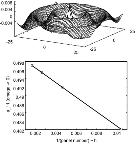
Figure 3 – Wave pattern on thez=0 plane caused by a square panel of lengthL =0.1, submerged at depth H =1 and pulsating at frequencyω(top). Convergence plot for the surge added mass of the unit hemisphere at very low frequencies (ω→0) obtained with a lineal regression analysis (exact A′11=1/2) (bottom).
5.2 Body coordinates and motions
bow
stern
X
Z
Y
ξ 4: roll ξ
1: surge
ξ 5: pitch
ξ 2: sway ξ
6: yaw ξ
3: heave
g
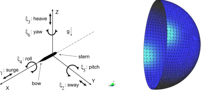
Figure 4 – Degrees of freedom with respect to the body coordinate system (left). Bound-ary mesh with 3 000 Kelvin panels over a hemisphere (right).
Hulme (1982) Papanikolau (1985)
D’33
11
A’
D’11
33
A’
384 panels
heave damping surge damping
surge added mass heave added mass
KR
KR KR
KR
96 panels
0 0.2 0.4 0.6
0 0.5 1 1.5 2
0 0.1 0.2 0.3
0 0.5 1 1.5 2
0 0.2 0.4 0.6
0 0.5 1 1.5 2
0 0.1 0.2 0.3
0 0.5 1 1.5 2
Figure 5 – Added massA′kkand damping coefficientsD′kkof the oscillating unit hemi-sphere, for surgek=1 or swayk =2 (left) and heavek =3 (right), as a function of the wave number coefficientK R.
5.3 Oscillating floating unit hemisphere
modes, it is not necessary to determine the sway mode, nevertheless, for a code validation, it was also verified at machine precision, in a perfectly symmetric mesh. The added mass coefficients are computed as A′kk = Akk/(ρV), and the
damping ones as Dkk′ = Dkk/(ρVω), whereV =(2/3)πR3is the hemisphere
volume,ρis fluid density andωis the imposed circular frequency. Figure 3 (bot-tom) shows a convergence plot for the surge added mass at very low frequencies (ω → 0), obtained with a lineal regression analysis (exact value A′11 = 1/2). The mesh is shown in Figure 4 (right) and has 3 000 Kelvin panels over the wetted body surface. Plots of the added mass A′kk and damping coefficients D′kk, as a function of the wave number coefficient K R, are shown for the surge and sway modes in Figure 5 (left), and for the heave mode in Figure 5 (right). All of them are in good agreement with the literature results [19]. The asymp-totic values of these coefficients, for very low and very high frequencies, can be obtained analytically, e.g. by variable separation or image methods. For the surge/sway mode at very low frequency, the boundary conditionφ,z = 0
is equivalent to a symmetry operation with respect to the plane z = 0 and, then, corresponds to the solution of a sphere oscillating in an infinite medium. The added mass for the last case is half of the displaced volume, then, the surge/sway added mass coefficient is A′11 = 1/2 with respect to the true displaced mass(2/3)πR3ρ, where the half factor is due to the analytic pro-longation. On the other hand, the asymptotic values of the added mass in heave mode are not easy to obtain and could be computed with spherical harmonics (e.g. see Storti-D’Elia [20]). Bounds for the surge A′11 and heave A′33 added mass coefficients of the oscillating unit hemisphere at very low and very high frequencies are summarized in Table 1. The first column corresponds to those found in Storti-D’Elia [20]. The values for the surge/sway mode in the sec-ond column correspsec-ond to those found in Sierevogel [21] and Prins [22], while the corresponding ones to the heave mode are taken from Korsmeyer [23] and Liapis [24]. It should be noted that only the intervals [0.25, 1.50] and [0.6, 1.5] were considered in Prins [22], respectively, and, then, the extrapolations are rather doubtful. The third column corresponds to the results found in Hulme [25].
[20] A′11from [21, 22] [25, 24] A′33from [23]
limK R→0A′11 0.5 0.5 0.5
limK R→∞A′11 0.272 220 012 593 0.25 … 0.273 239…
limK R→0A′33 0.830 949 128 536 0.80 … 0.830 951…
limK R→∞A′33 0.5 0.45 0.5
Table 1 – Added mass coefficients for surge/sway modeA′11and heave A′33one taken from the literature.
obtained with other panel methods with Kelvin kernels. In general, the concor-dance among the present results and the literature is good. Another validation test may include a comparison with related approaches found in the literature of ship engineering, such as those based on Chebyshev polynomials, e.g. the WAMIT software (http://www.wamit.com).
6 Conclusions
A semi-numerical scheme for computing the Kelvin kernel for seakeeping flow problems has been proposed. The Kelvin kernel is decomposed as the sum of two Rankine sources and a wave one. The Rankine sources are the standard Green functions for the Laplacian equation, one due to the generic panel on the body sur-face, placed below the planez =0, and the other one due to the mirror image with respect to the same plane. The wave kernel (i) tends to be ill-conditioned for field points near or over the local axisymmetric axis; and (ii) involves a rather heavy computation, due to the Haskind-Havelock integral which, in turn, involves the computation of Bessel and Strouve functions. The Haskind-Havelock integral was accurately computed with a singularity subtraction technique that involves a regular closed term and a numerical adaptive quadrature, while the Bessel and Strouve functions were calculated with asymptotic expansions. The proposed semi-numerical scheme was validated with analytical and semi-analytical so-lutions for the unit hemisphere in surge and heave motions, without showing numerical instabilities nor precision loss.
2009–III-4–2), Agencia Nacional de Promoción Científica y Tecnológica (AN-PCyT, Argentina, grants PICT 1506–06, PICT 1141–07 and PAE 22592–04 nodo 22961) and was performed with the Free Software Foundation/GNU-Project resources such as GNU–Linux OS, GNU–Gfortran and GNU–Octave, as well as other Open Source resources as Scilab, TGif, Xfig and LATEX. The authors thank the referees for their constructive suggestions and careful reading.
REFERENCES
[1] J.N. Newman, The theory of ship motions. Advances in Applied Mechanics,
18(1978), 221–285.
[2] J. Nossen, J. Grue and E. Palm, Wave forces on three-dimensional floating bodies with small forward speed.J. of Fluid Mechanics,227(1991), 135–160.
[3] S. Finne and J. Grue, On the complete radiation-difraction problem and wave-drift damping of marine bodies in the yaw mode of motion.J. of Fluid Mechanics,
357(1998), 289–320.
[4] R.F. Beck and W.C. Webster, Seakeeping and controllability. In: E.V. Lewis,
editor, Principles of Naval Architecture, volume III. SNAME (1989).
[5] F. París and J. Cañas, Boundary Element Method. Fundamentals and applications.
Oxford Press (1997).
[6] W. Hackbusch,Integral equations.Birkhäuser (1995).
[7] J. D’Elía, L. Battaglia, A. Cardona and M. Storti, Full numerical quadra-ture of weakly singular double surface integrals in Galerkin boundary element methods.Int. J. for Num. Meth. in Biomedical Engng.,27(2) (2011), 314–334. doi:10.1002/cnm.1309.
[8] F. Hartmann, Introduction to Boundary Elements.Springer-Verlag (1989).
[9] Y. Huang and P.D. Sclavounos,Nonlinear ship motions.J. of Ship Research,42(2) (1998), 120–130.
[10] D.C. Kring, Ship seakeeping through theτ =1/4critical frequency.J. of Ship
Research,42(2) (1998), 113–119.
[11] J.G. Telste and F. Noblesse,Numerical evaluation of the Green function of water-wave radiation and difraction.J. of Ship Research,30(2): 69–84, June (1986).
[13] F. Noblesse, The Green function in the theory of radiation and difraction of regular water waves by a body.J. of Engineering Mathematics,16(1982), 137– 169.
[14] J.N. Newman, Algorithms for the free-surface Green function.J. of Engineering
Mathematics,19(1985), 57–67.
[15] M. Abramowitz and I. Stegun, Handbook of Mathematical Functions. Dover (1972).
[16] D.E. Medina and J.A. Liggett,Three-dimensional boundary element computation of potential flow in fractured rock. Int. J. for Num. Meth. in Eng., 26 (1988), 2319–2330.
[17] J. D’Elía, M.A. Storti and S.R. Idelsohn, A closed form for low order panel methods.Advances in Engineering Software,31(5) (2000), 335–341.
[18] J. D’Elía, M.A. Storti and S.R. Idelsohn, Iterative solution of panel discretiza-tions for potential flows. The modal/multipolar preconditioning. Int. J. Num.
Meth. Fluids,32(1) (2000), 1–22.
[19] A. Papanikolau, On the integral-equation-methods for the evaluation of motions and loads of arbitrary bodies in waves.Ingenieur-Archiv,55(1985), 17–29.
[20] M.A. Storti and J. D’Elía, Added mass of an oscillating hemisphere at very-low and very-high frequencies.ASME, Journal of Fluids Engineering,126(6), 1048– 1053, November (2004).
[21] L. Sierevogel,Time-domain Calculations of Ship Motions.PhD thesis, Technische
Universiteit Delft (1998).
[22] H.J. Prins, Time-domain Calculations of Drift Forces and Moments.PhD thesis,
Technische Universiteit Delft (1995).
[23] F.T. Korsmeyer and P.D. Sclavounos, The large-time asymptotic expansion of the impulse response function for a floating body. Applied Ocean Research, 11(2) (1989), 75–88.
[24] S.J. Liapis, Time-domain Analysis of Ship Motions. PhD thesis, University of
Michigan (1986).