ISSN 0101-8205 www.scielo.br/cam
Dynamical behavior of a pest management model
with impulsive effect and nonlinear incidence rate*
XIA WANG1, ZHEN GUO2 and XINYU SONG1
1College of Mathematics and Information Sciences, Xinyang Normal University, Xinyang 464000, Henan, P.R. China
2School of Computer and Information Technology, Xinyang 464000, Henan, P.R. China
E-mail: [email protected]
Abstract. In this paper, we consider the pest management model with spraying microbial pesticide and releasing the infected pests, and the infected pests have the function similar to the microbial pesticide and can infect the healthy pests, further weaken or disable their prey function till death. By using the Floquet theory for impulsive differential equations, we show that there exists a globally asymptotically stable pest eradication periodic solution when the impulsive periodτ < τmax, we further prove that the system is uniformly permanent if the impulsive period
τ > τmax. Finally, by means of numerical simulation, we show that with the increase of impulsive period, the system displays complicated behaviors.
Mathematical subject classification: 34C05, 92D25.
Key words:pest-management model, impulsive effect, extinction, permanence.
1 Introduction
From the reports of Food and Agriculture Organization of the United Nations, the warfare between man and pests has lasted for thousands of years. With the
#CAM-192/10. Received: 10/III/10. Accepted: 28/IV/10.
development of society and progress of science and technology, there are many ways to control agricultural pests, for instance biological pesticides, chemical pesticides, remote sensing and measuring and so on. A great deal of pesticides were used to control pests. Generally speaking, pesticides are useful because they can quickly kill a significant portion of a pest population and sometimes provide the only feasible method for preventing economic loss. However, pes-ticides pollution is also recognized as a major health hazard to human beings and to natural enemies. Hence, many scholars put forward Integrated Pest Management (IPM) (see [1, 3, 4, 11]), IPM is a pest management system that in the context of the associated environment and the population dynamics of the pest species, utilizes all suitable techniques and methods in as a compatible manner as possible and maintains the pest populations at levels below those causing economic injury.
Recently, the models for pest control were studied by some authors ([2-6]) and some results were obtained. As we all know, most of the research literature on these epidemic models assumed that the disease incubation is negligible, so that, once infected, each susceptible individual(S)instantaneously becomes infectious (I) and later recovers(R)with a permanent or temporary acquired immunity. A model based on these assumptions is often called an SIR or SIRS model. The SIR epidemiological model was studied in [7], they assumed that the susceptible satisfied the logistic equation and the incidence rate was of the formk I Sq and the total population was not constant.
However, it is inevitable that IPM may cause pollution to the environment more or less due to the use of chemical pesticide. Therefore, in this paper we propose a biological control strategy-controlling the pest by introducing micro-bial pesticide and infected pests simultaneously. Compared with the chemi-cal pesticide, the application shows that the microbial pesticide is an effective, highly infectious and safe bio-pesticide which can be used in both short-term and long-term controls and plays an important role in pest management.
The model we consider is based on the following SI model:
˙
S= −βS(t)I(t), ˙
β > 0 is called the transmission coefficient, d > 0 is the death rate of the infectious pests.
For IPM strategy, we combine the biological control and chemical control. The infectious pests are released periodically every time periodτ, meanwhile periodic spraying the microbial pesticide for susceptible pests. Based on biolog-ical control strategy in pest management, we construct a pest-epidemic model with impulsive control. Impulsive differential equations found in almost every domain of applied science and have been studied in many investigations ([8-13]). But to our knowledge there are only a few papers and books on mathemat-ical model of the dynamics of microbial diseases in pest control. Li et al. [14], Anderson et al. [15] and Jong et al. [16] pointed out that standard incidence is more suitable than bilinear incidence. Levin et al. [17] have adopted a incidence form like βSlIh or βShIh
N , l > 0, h > 0 which depends on different infective
diseases and environment. So we develop (1.1) by introducing a constant peri-odic releasing of the infective pests and spraying microbial pesticides at fixed moment. That is, we consider the following impulsive differential equations:
˙
S(t)=r S
1− S+θI K
−βS Iq, ˙
I(t)=βS Iq−d I,
t
6=nτ, n ∈N,
1S= −(μ1+μ2)S, 1I =μ1S−μ3I +p,
t=nτ, n∈N,
(1.2)
2 Notations and definitions
In this section, we give some notations which will prove useful and give some definitions.
Let R+ = [0,∞), R+2 = {x ∈ R2: x > 0}, = intR2+, N be the set of
all nonnegative integers. Denote f = (f1, f2), the map defined by the right hand side of the first two equations of system (1.2). Let V0 = {V: R+ ×
R2
+7→ R+}, continuous on(nτ, (n+1)τ] ×R+2, and lim(t,y)→(nτ+,x)V(t,y)= V(nτ+,x)exists.
Definition 2.1. V ∈V0, then for(t,x)∈(nτ, (n+1)τ] ×R2
+, the upper right
derivative of V(t,x) with respect to the impulsive differential system (1.2) is defined as
D+V(t,x)=lim
h→0sup 1 h h
V(t+h,x+h f(t,x))−V(t,x)i.
The solution of system(1.2)is a piecewise continuous function x: R+7→ R2+,
x(t)is continuous on(nτ, (n+1)τ],n∈Nand x(nτ+)=limt→nτ+x(t)exists. Obviously the smoothness properties of f guarantee the global existence and uniqueness of solution of system(1.2), for details (see[18]).
We will use a basic comparison result from impulsive differential equations. For convenience, we state it in our notations.
Suppose g: R+×R+7→ R satisfies:
(H) g is continuous in(nτ, (n+1)τ] ×R+and for x∈ R+, n∈N,
lim(t,y)→(nτ+,x)g(t,y)=g(nτ+,x)exists.
Lemma 2.2. Let V ∈V0, assume that
D+V(t,x)≤g(t,V(t,x)), t6=nτ, V(t,x(t+))≤ψn(V(t,x(t))), t=nτ,
(2.1)
where g: R+×R+ 7→ R satisfies(H)andψn: R+ 7→ R+ is nondecreasing.
Let h(t)be the maximal solution of the scalar impulsive differential equation
˙
u(t)=g(t,u(t)), t6=nτ, u(t+)=ψn(u(t)), t=nτ,
u(0+)=u0
existing on[0,∞). Then V(0+,x0)≤u0implies that V(t,x(t))≤h(t),t ≥0, where x(t)is any solution of (1.2), similar result can be obtained when all the directions of the inequalities in the lemma are revered andψn is
nonincreas-ing. Note that if we have some smoothness conditions of g to guarantee the existence and uniqueness of solutions for(2.2), then h(t)is exactly the unique solution of(2.2).
Lemma 2.3. Suppose that x(t)is a solution of system(1.2)with x(0+) ≥ 0,
then x(t)≥0for all t ≥0. Further, if x(0+) >0, then x(t) >0for all t >0. For convenience, we give some basic properties of the following system
˙
I = −d I, t 6=nτ, 1I = −μ3I +p, t =nτ.
(2.3)
Then we have the following lemma:
Lemma 2.4. System (2.3) has a unique positive periodic solution eI(t) with periodτ and for every solution I(t) of(2.3) such that|I(t)−eI(t)| → 0 as t→ ∞, where
eI(t)= pexp(−d(t−nτ )) 1−(1−μ3)exp(−dτ )
, eI(0+)= p
1−(1−μ3)exp(−dτ ) andeI(t)is globally asymptotically stable. Hence the solution of(2.3)is
I(t)=(1−μ3)(eI(0+)−
pexp(−d(t−nτ ))
1−(1−μ3)exp(−dτ ))exp(−dt)+eI(t).
Lemma 2.5. There exists a constant M >0 such that S(t) ≤ M,I(t) ≤ M for each positive solution x(t)=(S(t),I(t))of(1.2)with all t large enough.
Proof. DefineV(t,x(t))= S(t)+I(t). ThenV(t,x(t)) ∈V0and the upper right derivative ofV(t,x(t))along solution of (1.2) is described as
D+V(t,x(t))+d V(t,x(t)) =(r +d)S(t)−r S 2(t)
K −
rθS(t)I(t) K ≤(r +d)S(t)−r S
where
L0= K(r +d) 2
4r ,
whent =nτ, we obtain
V(nτ+)=(1−μ2)S(nτ )+(1−μ3)I(nτ )+p≤V(nτ )+p. According to Lemma 2.2, fort∈(nτ, (n+1)τ ), we have
V(t,x(t)) ≤ V(0+)exp(−dt)+ Z t
0
L0exp(−d(t−s))ds
+ X
0<nτ <t
pexp Z t
nτ
(−d)ds
≤ V(0+)exp(−dt)+ L0
d (1−exp(−dt))
+pexp(−d(t−τ )) 1−exp(dτ ) +
pexp(μτ ) exp(dτ )−1
→ L0
d +
pexp(dτ )
exp(dτ )−1, t→ ∞.
Definition 2.6. System (1.2) is said to be permanent if there exists positive constants m,M such that each positive solution (S(t),I(t)) of system (1.2) satisfies m≤ S(t)≤ M,m ≤ I(t)≤ M for all t sufficiently large.
3 Stability of the pest-eradication periodic solution
In this section, we study the stability of the pest-eradication periodic solution of system (1.2).
Theorem 3.1. The pest-eradication periodic solution(0,eI(t))of system(1.2) is globally asymptotically stable provided
rτ− prθ (1−exp(−dτ )) d K[1−(1−μ3)exp(−dτ )] −
pqβ(1−exp(−qdτ ))
2d[1−(1−μ3)exp(−dτ )] <−ln(1−μ1−μ2).
Proof. Firstly, we prove the local stability of aτ-period solution(0,eI(t))may be determined by considering the behavior of small-amplitude perturbations (u(t), v(t))of the solution.
Define
S(t)=u(t), I(t)=v(t)+eI(t), whereu(t), v(t)are small perturbations, there may be written as
u(t) v(t) !
=8(t) u(0) v(0) !
where8(t)satisfy
d8(t) dt =
r −rθk eI(t)−βeIq(t) 0
βeIq(t) −d !
8(t),
where8(0) is the identity matrix. The resetting impulsive conditions of (1.2) becomes
u(nτ+) v(nτ+) !
= 1−μ1−μ2 0
μ1 1−μ3 !
u(nτ ) v(nτ ) !
.
Hence, if absolute values of all eigenvalues of
M = 1−μ1−μ2 0 μ1 1−μ3
! 8(τ ),
are less than one, theτ-periodic solution is locally stable. By calculating, we have
8(τ ) = 1−μ1−μ2 0 μ1 1−μ3
!
× exp
Z τ
0
r−rθ
KeI(t)−βeI
q
(t)
dt
0
∗ exp(−dτ )
,
following:
λ1=(1−μ1−μ2)exp Z τ
0
r −rθ
KeI(t)−βeI
q(t)
dt
,
λ2=(1−μ3)exp(−dτ ),
λ1 < 1 if (3.1) holds true. According to Floquet theory, the pest-eradication solution(0,eI(t))is locally asymptotically stable.
In the following, we prove the global attractivity. Choose a sufficiently small ε >0 such that
δ=(1−μ1−μ2)× exp
Z τ
0
r −rθ
K(eI(t)−ε)−β(eI(t)−ε)
q
dt
<1.
Noting that I˙(t) ≥ −d I(t) as t 6= nτ and 1I(t) ≤ −μ3I(t) + p as t=nτ, consider the following impulsive differential equation:
˙
x(t)= −d x(t), t 6=nτ,
1x(t)= −μ3x(t)+p, t =nτ, (3.2) by Lemma 2.4, system (3.2) has a globally asymptotically stable positive periodic solution
ex(t)= pexp(−d(t−nτ )) 1−(1−μ3)exp(−dτ ). So by Lemmas 2.2 and 2.4, we get
I(t)≥ x(t) >eI(t)−ε. (3.3)
From system (1.2), we obtain that
˙
S(t)≤ S(t)
r −rθ
K(eI(t)−ε)−β(eI(t)−ε)
q
, t6=nτ,
1S(t)= −(μ1+μ2)S(t), t=nτ.
Integrating (3.4) on(nτ, (n+1)τ], which yields
S((n+1)τ ) = S(nτ+)×
exp
Z (n+1)τ nτ
r −rθ
K(eI(t)−ε)−β(eI(t)−ε)
q
dt
= (1−μ1−μ2)S(nτ )× exp
Z (n+1)τ nτ
r −rθ
K(eI(t)−ε)−β(eI(t)−ε)
q
dt
= S(nτ )δ.
(3.5)
Thus, S(nτ ) ≤ S(0)δn and S(nτ ) → 0 asn → ∞. Therefore, S(t) → 0 as t→ ∞, since 0<S(t) < (1−μ1−μ2)S(nτ )exp(rτ )fornτ <t ≤(n+1)τ. Next, we prove that I(t)→eI(t)ast → ∞, for a sufficiently small 0< ε <
d
βMq−1, there exists a T1 > 0 such that 0 < S(t) < ε for allt > T1. From system (1.2), we have
˙
I(t)≤(βεMq−1−d)I(t), t6=nτ,
1I(t)≤μ1ε−μ3I(t)+p, t=nτ, (3.6)
considering the following comparison system
˙
y(t)=(βεMq−1−d)y(t), t6=nτ,
1y(t)=μ1ε−μ3y(t)+p, t=nτ. (3.7)
By Lemma 2.4, system (3.7) has a positive periodic solution
ey(t)= (μ1ε+ p)exp(−(d−βεM
q−1)(t−nτ ))
1−(1−μ3)exp(−(d−βεMq−1)τ ) , nτ <t≤(n+1)τ, which is globally asymptotically stable. Thus, for a sufficiently smallε1, there exists aT2>T1>0 such thatt>T2
4 Permanence
Theorem 4.1. System(1.2)is uniformly permanent if
rτ− prθ (1−exp(−dτ )) d K[1−(1−μ3)exp(−dτ )]
− p
qβ(1−exp(−qdτ ))
2d[1−(1−μ3)exp(−dτ )] >−ln(1−μ1−μ2).
(4.1)
Proof. Suppose x(t) = (S(t),I(t)) is a solution of (1.2) with x(0) > 0, from Lemma 2.5, we may assume S(t) ≤ M,I(t) ≤ M and M > (r/β)1q,
fortlarge enough.
Letm2= pexp(−dτ )
1−(1−μ3)exp(−dτ )−ε2, whereε2>0 sufficiently small. According to Lemmas 2.2 and 2.4, we have I(t) > m2 for t large enough. So, if we can find positive numberm1 > 0, such that S(t) > m1 fort large enough, then our aim is obtained.
Next, we will do it in the following two steps for convenience.
Step I: If (4.1) holds true, we can choose 0 < m1 < d
βMq−1 andε3 small enough such that
δ1=(1−μ1−μ2)× exp
Z (n+1)τ nτ
r −r m1 k −
rθ
k (eI(t)+ε3)−β(eI(t)+ε3)
q
dt
>1,
we will prove there exist a t1 ∈ (0,∞), such that S(t1) ≥ m1. Otherwise S(t) <m1for allt >0. From system (1.2), we obtain that
˙
I(t)≤(βm1Mq−1−d)I(t), t 6=nτ, 1I(t)≤μ1m1−μ3I(t)+p, t =nτ,
(4.2)
consider the following comparison system
˙
z(t)=(βm1Mq−1−d)z(t), t6=nτ,
by Lemmas 2.2 and 2.4 on (4.3), we havez(t)→ ˜z(t)ast → ∞, where
˜
z(t)= (μ1m1+p)exp(−(d−βm1M
q−1)(t−nτ )) 1−(1−μ3)exp(−(d−βm1Mq−1))
, nτ <t ≤(n+1)τ.
Therefore, there exists aT3>0 such that
I(t)≤z(t) <z(t˜ )+ε,
fort>T3. Thus
˙
S(t)≥ S(t)(r −r m1
K −
rθ K (
˜
I(t)+ε)−β(I˜(t)+ε)q), t 6=nτ, 1S(t)= −(μ1+μ2)S(t), t =nτ,
(4.4)
fort > T3, integrating (4.4) on(nτ, (n+1)τ], n ≥ N1, here N1is a nonneg-ative integer andN1τ ≥T3, then we obtain
S((n+1)τ ) ≥S(nτ )(1−μ1−μ2)
×exp
Z (n+1)τ nτ
r−r m1
K −
rθ
K(I˜(t)+ε)−β(I˜(t)+ε) q
dt !
=S(nτ )δ1.
ThenS((N1+k)τ ) ≥ S(N1τ )δk1 → ∞, k → ∞, which is a contradiction to S(t) <m1for allt >0. Hence there exists at1such thatS(t1)≥m1.
Step II: If S(t) ≥ m1 for all t ≥ t1, then our aim is obtained. Otherwise S(t) < m1 for some t ≥ t1, setting t∗ = inft>t1{S(t) < m1}, there are the
following two cases fort∗:
Case (a): Ift∗ = n1τ,n1 is some positive integer. In this case S(t) ≥ m1 fort ∈ [t1,t∗) and(1−μ1−μ2)S(t∗+) = (1−μ1−μ2)S(t∗) < m1. Let T4 = n2τ +n3τ, where n2 = n′2+n′′2, n′2,n′′2 and n3 satisfy the following inequalities:
n′2τ > 1
βm1Mq−1−d ln
ε3
(μ1m1+ p+M)(1−μ3) ,
(1−μ1−μ2)n2exp(ηn2τ )δ
n3
where
η=r−r m1
K −
rθ
K M−βM
q
<0.
We claim that there must be a time t2 ∈ (t∗,t∗+T4) such that S(t2) ≥ m1, if it is not true, i.e., S(t) < m1,t ∈ (t∗,t∗ + T4), similar to the analysis before, we consider system (4.3) with initial value z(t∗+) = I(t∗+) ≥ 0, by Lemma 2.4, we have
z(t) =(1−μ3)(z(t∗ +
)− p+μ1m1
1−(1−μ3)exp(−(d−βm1Mq−1)τ )) ×exp(−(d−βm1Mq−1)(t−t∗))+ ˜z(t)
fort∈(nτ, (n+1)τ], n1≤n ≤n1+n2+n3. Then
|z(t)− ˜z(t)|< (1−μ3)(M+p+μ1m1)exp(−(d−βm1Mq−1)(t−n1τ )) < ε3, and I(t) ≤ z(t) < z(t)˜ +ε3 fort∗ +n′2 ≤ t ≤ t∗+T4, which implies that system (4.4) holds for [t∗ + n2τ,t∗ +T4], integrating system (4.4) on this interval, we have
S((n1+n2+n3)τ )≥ S((n1+n2)τ )δn3
1 . (4.5)
In addition, we have ˙
S(t)≥S(t)
r −r m1
K −
rθ
K M−βM
q
=ηS(t),
1x1(t)=(1−μ1−μ2)x1(t).
(4.6)
Integrating system (4.6) on the interval[t∗, (n1+n2)τ], which yields
S((n1+n2)τ )≥m1(1−μ1−μ2)n2exp(ηn2τ ), (4.7) combining (4.5) and (4.7), we have
S((n1+n2+n3)τ )≥m1(1−μ1−μ2)n2exp(ηn2τ )δ
n3
1 >m1,
suppose t ∈ (t∗ +(l −1)τ,t∗ +lτ] ⊂ (t∗,tˆ], l is a positive integer and l ≤n2+n3, from system (4.6), we have
S(t) ≥(1−μ1−μ2)lm1exp(lητ )
≥(1−μ1−μ2)n2+n3exp((n2+n3)τ )=1 m1
for t > tˆ. The same arguments can be continued since S(t)ˆ ≥ m1. Hence S(t)≥m1for allt >t1.
Case (b): Ift∗ 6=nτ, then S(t∗)= m1andS(t) ≥ m1, t ∈ [t1,t∗], suppose t∗ ∈ (n′1τ, (n′1+1)τ], we also have two subcases for t ∈ [t∗, (n′1 +1)τ] as follows:
Case (i): S(t) ≤ m1, t ∈ [t∗, (n′1+1)τ], we claim that there exists at2′ ∈ [n′1τ, (n′1+1)τ+T4]such that S(t2′) >m1. Otherwise integrating system (4.6) on the interval[(n′1+1+n2)τ, (n′1+1+n2+n3)τ]produces
S (n′1+1+n2+n3)τ≥ S (n′1+1+n2)τδn3
1 .
SinceS(t)≤m1,t∈ [t∗, (n′1+1)τ], system (4.7) holds on[t∗, (n′1+1+n2+ n3)τ], thus
S (n′1+1+n2)τ = S(t∗)exp η (n′1+1+n2)τ −t∗(1−μ1−μ3)n2
≥ m1(1−μ1−μ3)n2exp(ηn2τ ) and
S (n′1+1+n2+n3)τ≥m1(1−μ1−μ3)n2+n3exp(ηn2τ )δn3
1 >m1, which is a contradiction. Let t˘ = inft>t∗{S(t) ≥ m1}, then S(t)˘ = m1 and S(t) <m1fort ∈(t∗,t)˘ . Chooset ∈(n′1τ +(l′−1)τ,n′1+l′τ] ⊂(t∗,t),˘ l′is a positive integer andl′<1+n2+n3, we have
S(t) ≥ ((n′1+l′−1)τ+)exp(η(t−(n′1+l′−1)τ )) ≥ (1−μ1−μ3)l′−1S(t∗)exp(η(t−t∗)) ≥ (1−μ1−μ3)n2+n3exp((n2+n3+1)ητ ),
Case (ii): If there exists a t ∈ (t∗, (n′1 +1)τ] such that S(t) ≥ m1. Let t = inft>t∗{S(t) ≥ m1}, then S(t) < m1 for t ∈ [t∗,t)and S(t) = m1. For t∈ [t∗,t), (4.6) holds and integrating (4.6) on[t∗,t), we have
S(t)≥ S(t∗)exp(η(t−t∗))≥m1exp(ητ ) >m1.
Since S(t) ≥ m1 fort > t, the same argument can be continued. Hence, we haveS(t) > m1for allt >t1. Thus in both cases, we concludeS(t) ≥ m1for allt ≥t1. The proof is complete.
Remark 1. Let
f(τ ) = rτ − prθ (1−exp(−dτ )) d K[1−(1−μ3)exp(−dτ )]
− p
qβ(1−exp(−qdτ ))
qd[1−(1−μ3)exp(−dτ )]q −ln(1−μ1−μ2).
Since f(0) = −ln1−μ1
1−μ2, f(τ ) → +∞ as τ → ∞ and f
′(τ ) > 0, so
f(τ ) = 0 has a unique positive root, denoted byτmax. From Theorem 3.1 and Theorem 4.1, we know that the pest-eradication periodic (0,eI(t)) is globally asymptotically stable whenτ < τmax. Ifτ > τmax, the system (1.2) is perma-nence.
Remark 2. If μ1 = μ2 = μ3 = 0, that is, we only choose the biological control, we can obtain that τ0 is the threshold and τmax > τ0, which implies that we must release more infected pest to eradicate the pests. If p = 0, that is there is no periodic releasing infective pests, so we can easily obtain that τ1 = −1r ln(1 −μ1 −μ2) is the threshold and τmax > τ1, it is obviously, impulsive releasing pests may lengthen the period of spraying pesticides and therefore reduce the cost of pests control.
5 Numerical analysis and conclusion
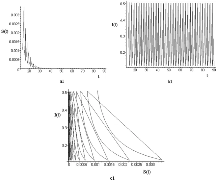
Figure 1 – Pest-eradication solution of system (1.2) which is globally asymptotically stable whenτ =1.5< τmax. (a1) Time series ofS(t)in (1.2) with initial value(0.1,0.1), (b1) Time series ofI(t)in (1.2) with initial value(0.1,0.1), (c1) Phase portraits in (1.2) with initial value(0.1,0.1).
Figure 2 – Dynamical behavior of system (1.2) withτ =3.5> τmax. (a2) Time series ofS(t)in (1.2) with initial value(0.1,0.1), (b2) Time series ofI(t)in (1.2) with initial value(0.1,0.1), (c2) Aτ-periodic solution.
It is observed that, theoretically speaking, the control strategy can be always made to succeed by the use of proper pesticides, while as far as the biological control is concerned, its sufficient effectiveness can also be reached provided that the numbers μi (i = 1,2,3) of infected pests released each time or the
periodτ is proper, that is, from Theorem 3.1 and Theorem 4.1, we know that the pest-eradication periodic (0,eI(t)) is globally asymptotically stable when τ < τmax (see Fig. 1). If τ > τmax, the system (1.2) is permanence (see Fig. 2). Any of these features alone can ensure the global success of our control strategy, although in concrete situations these may or may not be biologically feasible or may require a large amount of resources.
Figure 3 – Dynamical behavior of system (1.2) withτ =4.5>2τmax, (a3) Time series ofS(t)in (1.2) with initial value(0.1,0.1), (b3) Time series ofI(t)in (1.2) with initial value(0.1,0.1), (c3) Phase portraits in (1.2) with initial value(0.1,0.1).
θ =0.91, β =2, d =0.98, q =1.8, p =0.4, μ1=0.7, μ2=0.1, μ3 = 0.1, τmax=1.838045.
REFERENCES
[1] C.B. Huffaker,New technology of pest control.Wiley, New York (1980). [2] H.J. Barclay,Models for pest control using predator release, habitat management
and pesticide release in combination.J. Appl. Ecol.,19(1982), 337–348. [3] X. Wang and X.Y. Song,Analysis of an impulsive pest management SEI model
with nonlinear incidence rate.Computational & Applied Mathematics,29(2010), 1–17.
[4] S.Y. Tang, Y.N. Xiao, L.S. Chen and R.A. Cheke, Integrated pest management
[5] J.C. Van Lenteren,Integrated pest management in protected crops, in Integrated
Pest Management.D. Dent (Ed.), Chapman and Hall, London, (1995), 311–320.
[6] X. Wang and X.Y. Song,A predator-prey system with two impulses on the diseased
prey and a Beddington-DeAngelis response.Math. Meth. Appl. Sci.,33(2010),
303–312.
[7] X.A. Zhang and L.S. Chen,The periodic solution of a class of epidemic models.
Comput. Math. Appl.,38(1999), 61–71.
[8] X. Wang and X.Y. Song, Mathematical models for the control of a pest popu-lation by infected pest.Computers & Mathematics with Applications,56(2008), 266–278.
[9] Z. Agur, L. Cojocaru, R. Anderson and Y. Danon,Pulse mass measles
vaccina-tion across age cohorts.Proc. Natl Acad. Sci. USA,90(1993), 11698–11702.
[10] G. Ballinger and X.N. Liu, Permanence of population growth models with
impulsive effects.Math. Comput. Modelling,26(1997), 59–72.
[11] J.J. Jiao and L.S. Chen,A pest management SI model with periodic biological
and chemical control concern.Appl. Math. Comput.,183(2006), 1018–1026.
[12] H. Zhang and L.S. Chen, Pest management through continuous and impulsive
control strategies.BioSystems,90(2007), 350–361.
[13] X. Wang, Y.D. Tao and X.Y. Song,Mathematical model for the control of a pest
population with impulsive perturbations on diseased pest.Applied Mathematical
Modelling,33(2009), 3099–3106.
[14] Y.F. Li and X.Y. Song,Dynamic complexities of a Holling II two-prey one-predator system with impulsive effect.Chaos, solitons and Fractals,33(2007), 463–478. [15] R. Anderson and R. May,Infectious Diseases of Human: Dynamics and Control.
Oxford University Press (1991).
[16] M.C.M. De Jong, O. Diekmann and H. Heesterbeek,How does transmission
de-pend on population size? In: D. Mollison (Ed.), Human Infectious Diseases,
Epidemic Models, Cambridge University Press, Cambridge, UK (1995), pp. 84– 94.
[17] W.M. Liu, S.A. Levin and Y. Lwasa,Influence of nonlinear incidence rates upon
the behavior of SIRS Epidemiological models.J. Math. Biol.,25(1987), 359–380.