UNIVERSIDADE FEDERAL DO CEARÁ
CENTRO DE TECNOLOGIA
DEPARTAMENTO DE ENGENHARIA DE TRANSPORTES
PROGRAMA DE PÓS-GRADUAÇÃO EM ENGENHARIA DE TRANSPORTES
ANSELMO RAMALHO PITOMBEIRA NETO
DYNAMIC BAYESIAN STATISTICAL MODELS FOR THE ESTIMATION OF THE ORIGIN-DESTINATION MATRIX
FORTALEZA
ANSELMO RAMALHO PITOMBEIRA NETO
DYNAMIC BAYESIAN STATISTICAL MODELS FOR THE ESTIMATION OF THE ORIGIN-DESTINATION MATRIX
Tese de Doutorado apresentada ao Pro-grama de Pós-Graduação em Engenharia de Transportes do Departamento de Engen-haria de Transportes da Universidade Federal do Ceará como parte dos requisitos para a obtenção do título de Doutor em Engenharia de Transportes. Área de concentração: Plane-jamento e Operação de Sistemas de Trans-portes
Orientador: Prof. Dr. Carlos Felipe Grangeiro Loureiro
Dados Internacionais de Catalogação na Publicação Universidade Federal do Ceará
Biblioteca de Ciências e Tecnologia
P76d Pitombeira Neto, Anselmo Ramalho.
Dynamic bayesian statistical models for the estimation of the origin-destination matrix / Anselmo Ramalho Pitombeira Neto. – 2015.
102 f. : il.
Tese (doutorado) – Universidade Federal do Ceará, Centro de Tecnologia, Departamento de Engenharia de Transportes, Programa de Pós-Graduação em Engenharia de Transportes, Fortaleza, 2015.
Área de concentração: Planejamento e Operação de Sistemas de Transportes. Orientação: Prof. Ph.D. Carlos Felipe Grangeiro Loureiro.
1. Transportes - planejamento. 2. Teoria bayesiana de decisão estatística. I. Título.
Dedicado às mulheres da minha vida:
AGRADECIMENTOS
Ninguém faz nada sozinho. Embora este texto tenha sido redigido inteiramente por mim, este não deixa de ser um trabalho coletivo. Nessa caminhada de mais de quatro anos, contei com a ajuda e colaboração de muitas pessoas.
Primeiramente, gostaria de agradecer imensamente a Deus, pois Ele que nos dá força para seguir sempre em frente.
Ao meu orientador, Prof. Felipe Loureiro, por toda a dedicação e apoio.
À minha esposa Renata, por estar sempre ao meu lado e por me dar conforto nos momentos mais difíceis.
À minha mãe Rosa, minha irmã Camila, minha sobrinha Júlia e a todos os meus familiares, os quais sempre desejaram o melhor para mim.
Aos meus sogros, Crisóstomo e Neide, e a toda a família da minha esposa, a qual também se tornou a minha família.
“Whenever a theory appears to you as the only possible one, take this as a sign that you have neither understood the theory, nor the problem which it was intended to solve.”
ABSTRACT
In transportation planning, one of the first steps is to estimate the travel demand. A product of the estimation process is the so-called origin-destination matrix (OD matrix), whose
entries correspond to the number of trips between pairs of zones in a geographic region in a reference time period. Traditionally, the OD matrix has been estimated through direct methods, such as home-based surveys, road-side interviews and license plate automatic recognition. These direct methods require large samples to achieve a target statistical error, which may be technically or economically infeasible. Alternatively, one can use a statistical model to indirectly estimate the OD matrix from observed traffic volumes on links of the transportation network. The first estimation models proposed in the literature assume that traffic volumes in a sequence of days are independent and identically distributed samples of a static probability distribution. Moreover, static estimation models do not allow for variations in mean OD flows or non-constant variability over time. In contrast, day-to-day dynamic models are in theory more capable of capturing underlying changes of system parameters which are only indirectly observed through variations in traffic volumes. Even so, there is still a dearth of statistical models in the literature which account for the day-to-day dynamic evolution of transportation systems. In this thesis, our objective is to assess the potential gains and limitations of day-to-day dynamic models for the estimation of the OD matrix based on link volumes. First, we review the main static and dynamic models available in the literature. We then describe our proposed day-to-day dynamic Bayesian model based on the theory of linear dynamic models. The proposed model is tested by means of computational experiments and compared with a static estimation model and with the generalized least squares (GLS) model. The results show some advantage in favor of dynamic models in informative scenarios, while in non-informative scenarios the performance of the models were equivalent. The experiments also indicate a significant dependence of the estimation errors on the assignment matrices.
LIST OF FIGURES
Figure 1 – The traffic assignment problem . . . 28
Figure 2 – The OD matrix estimation problem . . . 28
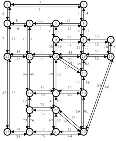
Figure 3 – Network used in the illustrative example . . . 54
Figure 4 – Simulation of OD flow in pair 1 . . . 56
Figure 5 – Simulation of OD flow in pair 2 . . . 56
Figure 6 – Simulation of OD flow in pair 3 . . . 57
Figure 7 – Simulation of volume on link 1 . . . 57
Figure 8 – Simulation of volume on link 2 . . . 58
Figure 9 – Simulation of volume on link 3 . . . 58
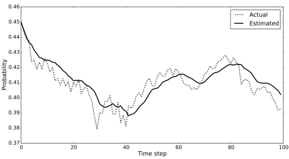
Figure 10 – Probability of choosing the route 1 in OD pair 2 . . . 59
Figure 11 – Schematic representation of Sioux Falls network . . . 61
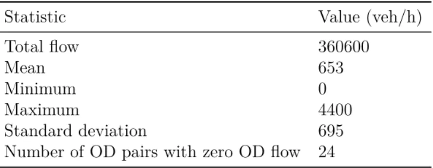
Figure 12 – Histogram of Sioux Falls OD flows . . . 62
Figure 13 – Congested links in Sioux Falls network (in black) . . . 63
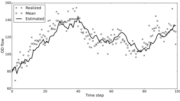
Figure 14 – Estimation of flows in OD pair 10-16 (high flow) by the dynamic estimation model . . . 69
Figure 15 – Estimation of flows in OD pair 10-16 (high flow) by the GLS model . . 70
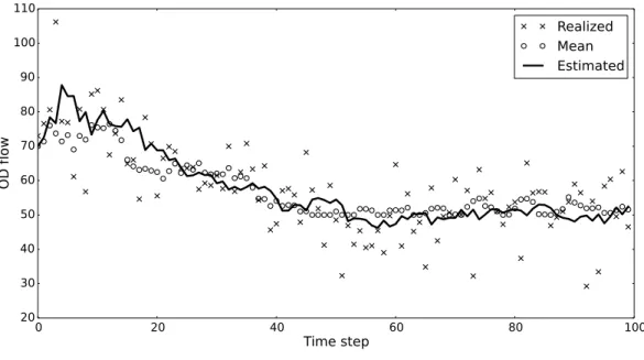
Figure 16 – Estimation of flows in OD pair 1-10 (medium flow) by the dynamic estimation model . . . 70
Figure 17 – Estimation of flows in OD pair 1-10 (medium flow) by the GLS model . 71 Figure 18 – Estimation of flows in OD pair 24-4 (low flow) by the dynamic estimation model . . . 71
Figure 19 – Estimation of flows in OD pair 24-4 (low flow) by the GLS model . . . 72
Figure 20 – Estimation of flows in OD pair 10-16 (high flow) by the dynamic model in the non-informative case . . . 72
Figure 21 – Estimation of flows in OD pair 10-16 (high flow) by the GLS model in the non-informative case . . . 73
Figure 22 – Estimation of link volumes in link 32 by the dynamic model . . . 73
LIST OF TABLES
Table 1 – Main characteristics of Sioux Falls network . . . 61
Table 2 – Statistics for the OD matrix of Sioux Falls . . . 62
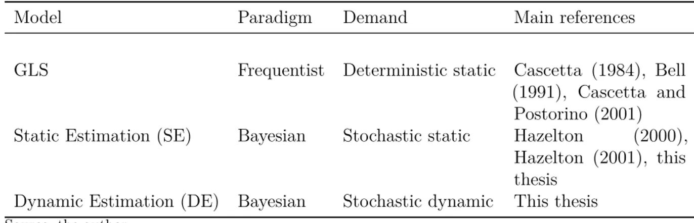
Table 3 – Main features of the tested models . . . 64
Table 4 – Parameters in the generation of simulated data . . . 66
Table 5 – Controlled parameters (kept constant) for the dynamic and GLS models in the test cases . . . 68
Table 6 – Cases studied in the computational experiment 1 . . . 68
Table 7 – Results for the application of the models to the Sioux Falls Network in the computational experiment 1 . . . 69
Table 8 – Controlled parameters (kept constant) for the models in the test cases in experiment 2 . . . 75
Table 9 – Cases studied in the computational experiment 2 . . . 75
Table 10 – Results for the application of the models to the Sioux Falls Network in the computational experiment 2 . . . 76
Table 11 – Effect of the assignment matrix on the estimation errors in experiment 3 76 Table 12 – OD matrix of the Sioux Falls network . . . 89
LIST OF ABBREVIATIONS AND ACRONYMS
OD Origin-destination
GLS Generalized least squares
ME Maximum entropy
DLM Dynamic linear model
MCMC Markov chain Monte Carlo
SE Static estimation
DE Dynamic estimation
MVN Multivariate normal distribution
MAP Maximum a posteriori
RMSE Root mean square error
RRMSE Relative root mean square error
MAE Mean absolute error
LIST OF SYMBOLS
x Vector of origin-destination (OD) flows.
y Vector of route flows.
z Vector of traffic volumes on links.
θ Vector of mean OD flows.
λ Vector of mean OD route flows.
p Vector of route choice probabilities.
c Vector of route costs.
¯
m Mean vector of the prior distribution in a DLM.
¯
C Covariance matrix of the posterior distribution in a DLM.
m Mean vector of the posterior distribution in a DLM.
C Covariance matrix of the posterior distribution in a DLM.
Ki Set of routes for OD pair i.
ξ Logit scale parameter.
π Probability of not using a route in the given route choice set.
κ Coefficient of variation.
τ Performance (cost) function of a link.
ν Vector of random errors in the measurement equation of a DLM.
ω Vector of random errors in the system equation of a DLM.
Σ A covariance matrix.
P Route choice matrix.
∆ Link-path incidence matrix.
A Adjustment matrix in the updating equations of a DLM.
F Assignment matrix/Regression matrix in DLM models.
W Covariance matrix of the mean OD flows (Evolution matrix).
I The identity matrix.
1 A vector full of scalars equal to one.
E[x] The expected value of the random variable x.
Var(x) The variance of the random variablex.
Cov(x, y) The covariance between random variables x and y.
diag(x) A matrix whose main diagonal is the vector xand entries off the main
diagonal are all zero.
blockdiag(Xi) A block-diagonal matrix composed of submatrices Xi
⌈x⌉ The smallest integer greater than x.
N(µ,Σ) Multivariate normal distribution with mean vector µ and covariance
matrix Σ.
CONTENTS
1 INTRODUCTION . . . 15
1.1 The problem . . . 15
1.2 Research gap . . . 16
1.3 General objective . . . 18
1.4 Specific objectives . . . 18
1.5 Structure of this doctoral thesis . . . 18
2 TRAFFIC ASSIGNMENT . . . 20
2.1 Modelling transportation flows on networks . . . 20
2.2 Route choice models . . . 21
2.3 Proportional assignment . . . 23
2.4 Equilibrium assignment . . . 24
3 ORIGIN-DESTINATION MATRIX ESTIMATION . . . 28
3.1 Problem description . . . 28
3.2 Models for the reconstruction of the OD matrix. . . 29
3.2.1 Maximum entropy . . . 30
3.2.2 Generalized least squares . . . 31
3.2.3 Maher’s Bayesian model . . . 32
3.2.4 Equilibrium-based models and the bilevel approach . . . 33
3.3 Models for the estimation of the mean static OD matrix . . . 36
3.3.1 Maximum likelihood . . . 36
3.3.2 Moment-based models . . . 38
3.3.3 Bayesian inference . . . 39
3.4 Models for the estimation of the dynamic OD matrix. . . 41
4 A BAYESIAN DYNAMIC LINEAR MODEL FOR THE DAY-TO-DAY ESTIMATION OF THE OD MATRIX . . . 44
4.1 Mathematical formulation of the model. . . 44
4.2 Updating equations for the formulated model . . . 48
4.3 Congestion and the estimation of route choice probabilities . . . 50
4.4 The static equilibrium-based case . . . 51
4.5 An illustrative example . . . 54
5 COMPUTATIONAL EXPERIMENTS . . . 60
5.1 Implementation details . . . 60
5.2 Characterizarization of the test network . . . 60
5.3 Tested models . . . 62
5.3.2 Static estimation model . . . 64
5.3.3 Dynamic estimation model . . . 64
5.4 Performance measures . . . 64
5.5 Generation of synthetic data . . . 65
5.6 Experiment 1 . . . 67
5.7 Experiment 2 . . . 70
5.8 Experiment 3 . . . 74
5.9 Comments on the main results . . . 77
6 CONCLUSION . . . 79
APPENDIX A – THE MULTIVARIATE NORMAL PROBABILITY DENSITY . . . 83
APPENDIX B – BAYESIAN INFERENCE . . . 84
APPENDIX C – DYNAMIC LINEAR MODELS . . . 85
ANNEX A – OD MATRIX OF SIOUX FALLS NETWORK . . . 89
ANNEX B – SIOUX FALLS NETWORK PARAMETERS . . . 94
15
1 INTRODUCTION
1.1 The problem
In transportation planning, one of the first steps is to estimate the travel demand. Generally, the demand is measured in terms of trip flows between zones in a geographic region. The final product of the estimation process is a so-called origin-destination matrix (OD matrix, for short), whose entries correspond to the number of trips between pairs of zones in a reference time period.
Traditionally, the OD matrix has been estimated through direct methods, such as home-based surveys, road-side interviews and license plate automatic recognition. These methods collect sample data on the number of trips performed daily, their origins and their destinations. Such data can be compiled and several statistics may be computed, such as the mean, standard deviation and confidence intervals. However, these direct methods require large samples to achieve a target statistical significance, which may be technically or economically infeasible (CASCETTA, 2009).
Another way of estimating the OD matrix is by using trip generation and dis-tribution models. In this approach, social and economic data are used to estimate the number of trips produced and attracted by each zone. In the next step, a gravity-type model is applied in order to distribute the generated trips between zones (ORTÚZAR; WILLUMSEN, 2011). Nevertheless, this approach also has its drawbacks. First, obtaining all the required data demands considerable amounts of resources, with high accompanying costs. Second, these models are in general aimed at long term planning horizons, which limit their use in short term applications, such as traffic management systems and public transit operation.
In the 1970s, researchers started developing alternative mathematical models whose objective was to obtain an OD matrix from indirect data on trip patterns. The main sources of indirect data were traffic volumes observed on links of the transportation network (also called traffic counts). The development of traffic monitoring systems opened up the possibility of acquiring data on traffic volumes in an automated way at low costs. In road networks this acquisition takes place by means of sensors installed on the roads, and in transit networks data on traffic of passengers can be acquired by means of electronic ticketing.
The rationale of these alternative models is to estimate OD flows through a mathematical model which relates traffic volumes on links of the transportation network to OD flows between zones. The models are in general of an optimization or statistical nature. The OD matrix so obtained is called a synthetic OD matrix, since it is not estimated by
Chapter 1. Introduction 16
evident: the transportation demand patterns in a part or in a whole region may be, in theory, traced to a finer time scale of days or hours, or even in real time. This is a great improvement over household surveys, which are typically carried out once in a decade, a time period during which the demand pattern may have changed considerably.
Since the pioneering work of Robillard (1975), many models have been proposed based on different approaches and assumptions. However, there are several issues related to the problem which have yet to be resolved satisfactorily, both from the theoretical and practical perspectives. Moreover, the literature lacks thorough comparisons and assessments of the performance and properties of the estimates produced by the alternative models. All this has led to a low adoption of the synthetic OD matrix based on link counts as an alternative to the more traditional and costly OD matrix obtained by means of direct estimation.
1.2 Research gap
The first attempts at estimating OD matrices from traffic counts relied on a single sample of volumes. The early data collection procedures involved the manual counting of vehicles in selected points in a transportation network. Due to technological or economical limitations, it was infeasible to take repeated samples of traffic volumes. Since there were no further data on traffic variability, a static and deterministic approach to the problem seemed plausible. The availability of a single sample of volumes provided only a snapshot of the transportation system in a point in time. The so-called reconstruction models sought to estimate mean OD matrices based on a sample of a single day. The validity of static reconstruction models critically hinged on the assumption that observed volumes were representative of a typical day.
More recently, many cities around the world have built traffic control systems, thereby massive data on urban traffic volumes have been collected daily. This opened up the possibility of applying statistical models based on large samples in order to estimate OD matrices and other relevant parameters more accurately. These first estimation models, initially proposed in the 1990’s, assume that traffic volumes in a sequence of days are independent and identically distributed samples of a static probability distribution. They use frequentist or Bayesian statistical techniques so as to estimate static quantities, such as mean OD matrices, variances of OD flows, or parameters of the route choice model.
A major weakness of static estimation models is that they do not allow for variations in mean OD flows or heteroscedasticity (i.e., non-constant variability) over time. In the relevant literature, two types of dynamics are often distinguished: within-day and day-to-day dynamics. Within-day dynamics refer to the temporal variation of the transportation
Chapter 1. Introduction 17
often of interest in short-term operational planning, since knowledge of the demand profile is valuable to effective intervention or to designing traffic management policies. In contrast, day-to-day dynamics is related to the variation of the demand for a repeated reference time period (typically the peak hour) over a sequence of days. It is more adequate for mid to long-term planning, when factors such as seasonality, changes in transportation supply and in economic activities are more pronounced. In this thesis, we focus on day-to-day dynamics.
In comparison with static models, day-to-day dynamic models are in theory more capable of capturing underlying changes of system parameters which are only indirectly observed through variations in traffic volumes. They may be more responsive to temporal changes and provide useful information on the dynamic behavior of the transportation system. Despite these promising features, there is still a dearth of statistical models in the literature which account for the day-to-day dynamic evolution of transportation systems.
Moreover, an important issue that we should be aware of when developing models for the estimation of the OD matrix is the occurrence of non-identifiability of the parameters, which refers to the existence of multiple parameter values which fit the data almost equally well. This issue has the implication that, except in very small transportation networks, it is often difficult to estimate OD matrices and other parameters based solely on traffic volume data. Some of the strategies to tackle this problem are: the development of parsimonious models, which are economic in the number of parameters; the use of a prior OD matrix, which can be, for example, an outdated matrix obtained by survey; or the adoption of simplifying and, in some cases, very restrictive assumptions.
In order to contribute to the development and analysis of day-to-day dynamic models for the OD matrix estimation problem, we propose a dynamic model and evaluate its potentials and limitations through computational experiments. Our main hypothesis is that day-to-day dynamic models can produce better estimates of mean OD matrices than static estimation models, since they should be able to account for the evolution of transportation systems over time and make use of the information provided by temporal changes. Our efforts are driven mainly towards attempting to answer the following specific questions:
• Are dynamic models capable of reducing the non-identifiability of mean OD matrices by incorporating the variation of the link volumes over time?
• Can dynamic estimation models produce better estimates of mean OD matrices than static estimation models?
• What is the impact of prior information on estimation errors?
Chapter 1. Introduction 18
According to the aforementioned research questions, the research objectives of this doctoral thesis are the following:
1.3 General objective
To assess the potential gains and limitations of day-to-day dynamic Bayesian statistical models for the estimation of the OD matrix based on link volumes.
1.4 Specific objectives
• To describe the main static and dynamic OD matrix estimation models currently
available in the literature;
• to propose a model for the estimation of the day-to-day dynamic OD matrix based on the theory of dynamic linear models;
• to perform computational experiments in order to evaluate the potential application of dynamic models relative to static models proposed in the literature;
• to assess how assignment matrices affect estimation errors, and
• to assess the impact of prior information on estimation errors.
1.5 Structure of this doctoral thesis
The literature review of our research is compiled in Chapters 2 and 3. We start by describing the traffic assignment models in Chapter 2. As we will see in Chapter 3, the OD matrix estimation problem is the inverse of the traffic assignment problem. Hence, many OD matrix estimation models embed traffic assignment models as part of their solution procedures. We describe the main variables and mathematical relationships involved in modeling transportation networks and the modeling of user behavior through route choice models. The traffic assignment models are presented according to the classification in proportional and equilibrium models, which correspond, in general, to assignment in uncongested and congested networks respectively.
Chapter 1. Introduction 19
20
2 TRAFFIC ASSIGNMENT
2.1 Modelling transportation flows on networks
Let (N,A) be a transportation network, in which N is a set of nodes and A is a set of directed links. Typically, for road networks, the links and nodes correspond to road segments and intersections between road segments, respectively. The transport network connects zones of a certain geographic region (e.g., a city), which “produce and attract”
trips, so that there is also a set of zones, denoted by I. A trip is a movement of a user
(person, freight, or vehicle) between an origin zone and a destination zone (referred to
simply as an OD pair). All trips enter and exit the network through centroid nodes, which
are terminal nodes located at zone centroids. Intrazonal trips are not taken into account, since their origin and destination centroid nodes coincide.
We denote by xi the total flow of trips in an OD pair i for a given time period.
In applications, a time period may be, e.g., the morning peak hour or a whole business day. What is traditionally meant as an OD matrix is a two-dimensional array whose row
indices identify origin zones, column indices identify destination zones, and the entries are the number of trips in an OD pair. As a matter of analytical convenience, in our notation the OD matrix is stretched out as a vector x∈Rn
+, for whichn = |I| is the number of
OD pairs. The total count of trips which flow through a link a for a given time period is denoted as the traffic volume za. The traffic volumes on all links are represented by a
vector z∈Rm+, and m=|A| is the number of links in the network.
For a given OD pair i, there is a set of routes connecting its origin and destination
zones. A route is a simple path between a pair of nodes. In general, we consider only a
reduced set of routes, since the total number of routes may be prohibitively large in real scale networks. (See Bekhor, Ben-Akiva and Ramming (2006) for an evaluation of route choice set generation algorithms). Let Ki be a set of routes associated with OD pair i. For
a route k ∈ Ki, we define yik as the flow of trips through route k in the reference time
period. Let also y∈Rr+ be the vector whose components are yik, and r=Pi∈I|Ki| is the
number of routes over all OD pairs.
Flows in OD pairs, route flows and traffic volumes are all related by flow conservation equations (2.1) and (2.2), given below:
X
k∈Ki
yik =xi ∀i∈ I (2.1)
za=
X
i∈I
X
k∈Ki
δakyik ∀a∈ A (2.2)
In equation (2.2), δak takes the value 1 if link a is part of route k, and 0 otherwise. It
Chapter 2. Traffic assignment 21
equation (2.2) in matrix notation, in which ∆= [δak]m×r is called thelink-path incidence
matrix:
z =∆y (2.3)
It is also worth defining the route choice fraction pik = yik/xi, which gives the
proportion of users in OD pair i that chooses to follow route k. Notice that it is possible
to establish a direct relationship between OD flows and traffic volumes through the route fractions. Let P= [pik]r×n be aroute choice matrix, then:
z =∆Px (2.4)
The route choice matrixPis commonly specified by means of a route choice model,
which estimates the probability that a user chooses a route as a function of the travel time (or generalized cost) associated with the route. Deterministic route choice models assume that the users have perfect knowledge of costs and always choose the route with minimum cost. In contrast, stochastic models assume that perceived costs of the users are
different from actual costs, so that they may choose routes which do not have minimum costs. The probabilities are estimated by means of discrete choice models, among which the multinomial logit and probit are the most used (CASCETTA, 2009).
The termF=∆Pis called theassignment matrix (CASCETTA; NGUYEN, 1988),
through which the relationship between xand z may be directly expressed by:
z =Fx (2.5)
As we will see in the forthcoming chapters, the assignment matrix plays a key role both in traffic assignment as in the OD matrix estimation problem.
2.2 Route choice models
Route choice models try to capture the choice behavior of users on which route to follow when going from an origin to a destination. Each route has a cost associated to it, and it is assumed that a user chooses the one route with minimum cost (rational behavior). Most of the occasions, costs will be measured in terms of travel time spent from origin to destination by following the chosen route. Other sources of costs may include, e.g., the gas consumption, toll fees or transit fares. In reality, all those may be aggregated in a
Chapter 2. Traffic assignment 22
It is assumed that the cost associated with a particular route depends linearly on the costs associated with the links that make up the route. Let ck be the cost associated
with a routek ∈ Ki for an OD pair i, and letτa be the cost associated with a linka. Then:
ck =
X
a∈A
δakτa+cN Ak k∈ Ki (2.6)
In equation 2.6, the term cN A
k corresponds to some fixed cost incurred when using the
route, e.g., a toll fee. Without loss of generalization, we assume it to be zero henceforth. Let pk = yk/xi be the fraction of trips in od pair i that flows through route k ∈ Ki,
withP
i∈Kipk = 1, andpk is a function of the route costs cj for all j ∈ Ki for OD pair i. There are two classes of models to determine the value of pk: Deterministic and stochastic
(CASCETTA, 2009).
In deterministic models, it is assumed that the user knows with certainty the costs associated to each route. Let c∗ = min
k∈Ki(ck) be the minimum cost among all routes in OD pair i. Thus:
pk =
1 ifck=c∗
0 ifck> c∗
∀k ∈ Ki (2.7)
In other words, the determination of pk by means of equation (2.7) implies that all trips in
OD pair iwill flow through the minimum cost route. In case there are multiple routes with
minimum cost, pk is undefined, since users will show no preference for a particular route.
A procedure to define a unique value for pk based on entropy maximization is presented in
(LARSSON et al., 2001).
On the other hand, in stochastic models, it is assumed that users do not have full knowledge of the actual costs associated with links and routes. In this way, the user chooses the route of minimum perceived cost, which is modelled as a random variable,
whose probability distribution captures the variability in perception among users. The route cost ck is then given by the following expression:
ck =
X
a
δakτa+cN Ak +ǫk (2.8)
The term P
aδkca+cN Ak is called systematic cost or actual cost associated with the route,
and the term ǫk corresponds to random error, which represents the variability in the
perceptions of users with respect to actual cost. The fraction pk in stochastic models
Chapter 2. Traffic assignment 23
probability of k being a route with minimum cost:
pk= Prob(ck≤cl, ∀l 6=k) (2.9)
The determination ofpkin stochastic models depends on the probability distribution
of the error ǫk. Some of the models widely applied in the literature are theprobit, which
assumes a normal distribution, and the logit, which assumes a Gumbel distribution
(BEN-AKIVA; LERMAN, 1985). In the case of the probit model, pk must be estimated through
Monte Carlo simulation, while for the logit model, there is an analytical solution given in equation (2.10):
pk =
exp(−ck/ξ)
P
l∈Kiexp(−cl/ξ)
(2.10)
In equation (2.10), ξ is a scaling factor proportional to the variance of the error term ǫk.
An important issue in route choice models is the generation of theroute choice set.
Ideally, the models should consider exhaustively all available routes, but the number of routes in real networks is prohibitively large, which poses computational challenges in the development of efficient algorithms. This difficulty has been addressed in two directions: one consider the generation of a reduced choice set, by means of some criterion or procedure which samples meaningful routes from the point of view of the user (BEKHOR; BEN-AKIVA; RAMMING, 2006); the other consider the development of algorithms which do not require the enumeration of routes, such as Dial’s Algorithm (DIAL, 1971) and the algorithms proposed by Akamatsu (1996) and Bell (1995).
2.3 Proportional assignment
The earlier approaches to traffic assignment considered that congestion effects on costs were negligible, so that costs could be treated as constants independent of traffic link flows. The methods based on this assumption were called proportional traffic assignment,
since scaling the OD matrix by a constant would result in link flows scaled by the same constant. Proportional assignment procedures are generally classified in deterministic and stochastic, according to the corresponding route choice model adopted (See section 2.2).
A simple deterministic assignment method is the all-or-nothing (SHEFFI, 1985).
Chapter 2. Traffic assignment 24
algorithm is very convenient, by virtue of its computational efficiency and the fact that it can generate multiple routes at a time (AHUJA; MAGNANTI; ORLIN, 1993). The main drawback of the all-or-nothing procedure is that it is not much realistic. In real situations, the trips are distributed among multiple routes between each OD pair, instead of only one. Notwithstanding this limitation, the all-or-nothing procedure is still useful in intermediate steps in more sophisticated assignment procedures, as in equilibrium assignment.
In contrast, stochastic assignment procedures assign flows to multiple routes for an OD pair. They are based on stochastic route choice models, as the multinomial logit or probit. In summary, the procedure consists in computing the probabilities of each route, and then applying flow conservation equations (2.1) and (2.2) in order to determine route and link flows. The main issue in applying stochastic assignment is the generation of the route choice set. For a given OD pair, the number of possible routes in a real scale network can be overwhelmingly large, so that the enumeration of all possible routes may be infeasible, as already pointed out in Section 2.2.
As stated in the beginning of this Section, proportional assignment is more suitable for networks where congestion effects are negligible. In the next section we present a class of non-proportional assignment procedures, equilibrium methods, which take congestion into account.
2.4 Equilibrium assignment
From a practical point of view, proportional assignment models are useful only for networks with low to moderate congestion levels. Nevertheless, as flows increase in the network, so does congestion, and costs are significantly affected by it. Users respond to changes in costs by changing their routes, trying to minimize their private costs. By its turn, the route choices made by users determine traffic flows on routes and links, affecting back the costs of routes. This feedback loop makes the whole transportation network behave as a dynamic system. Ceteris paribus, the transportation network may eventually reach an
equilibrium state in the long run, in which the flows remain constant over time. We refer to equilibrium traffic assignment as the determination of traffic flows for a network in an equilibrium state for a given OD matrix.
One of the first definitions of traffic equilibrium is known asWardrop first principle,
whose statement is: in Wardrop equilibrium, “The journey times on all the routes actually
used are equal, and less than those which would be experienced by a single vehicle on any unused route.” (WARDROP, 1952, p. 345).
In mathematical terms, in a Wardrop equilibrium, for any two routes k and l:
Chapter 2. Traffic assignment 25
When a transportation network is at Wardrop equilibrium, no user has incentive to unilaterally change route because all other routes have cost equal to or greater than the route currently used. Devarajan (1981) shows that this is equivalent to the definition of Nash equilibrium in non-cooperative games. Although a Wardrop equilibrium is reached as users try to optimize their particular costs, it is not necessarily optimal to the user, as there may be traffic distributions that produce lower costs for all users, as is demonstrated by the so-called Braess paradox (BRAESS; NAGURNEY; WAKOLBINGER, 2005). There may also be a traffic distribution which is socially optimal, in which the sum of costs of all users is minimum (this is known in the literature as Wardrop second principle).
Equilibrium assignment relies on linkperformance functionsin order to evaluate the
effect of congestion on links. In general, as traffic volumes increase, so do the time spent on links, the consumption of gas by vehicles, and other proxies of cost. The dependence of costs on link flows is modelled by the performance functions, among which the BPR function is very popular in the transportation theory and practice, given below (CASCETTA, 2009):
τa(za) =τa0
1 +α
za
zmax
a
!β
(2.12)
Where τa(za) is the cost in link a when there is a flow of za. The cost in “free flow” is
denoted as τa0, i.e., the cost the user incurs if no other user is using the link, andzamax is
the capacity of the link. α and β are parameters of the function (typical values adopted in
the literature are 0.15 and 4, respectively). Note that the capacity of the link is not treated as a hard constraint, i.e., actual volumes are allowed to be greater than the theoretical maximum. It is also worth noting that BPR function (equation (2.12)) has the following properties: it is continuous; it is strictly increasing, which means cost always increases with flow; and it is separable, which means the link costs depend solely on the flow on that link.
Smith (1979) has shown that a Wardropian equilibrium point satisfies the following variational inequalities with respect to link costs and flows:
τ(z∗)T(z−z∗)≥0 (2.13)
In equation 2.13, τ(z) is the vector of link costs, z is the vector of link flows, and z∗ is
the vector of equilibrium link flows. The satisfaction of inequalities (2.13) are also shown to be sufficient for the existence, uniqueness and stability of a Wardropian equilibrium point if the cost functions are continuous and strictly increasing. (BPR function, equation (2.12), satisfies both conditions).
Chapter 2. Traffic assignment 26
proposed by Beckmann, McGuire and Winsten (1956):
min X
a∈A
Z za
0 τa(v)dv (2.14)
s.t.
X
k∈Ki
yk =xi ∀i∈I (2.15)
za =
X
i∈I
X
k∈Ki
δakyk ∀a∈ A (2.16)
yk≥0 ∀k∈ Ki ∀i∈ I (2.17)
The objective function in (2.14) in known as Beckmann’s transformation, and has no
physical meaning. The constraints (2.15) and (2.16) are the flow conservation equations and (2.17) are non-negativity constraints on route flows. The mathematical program given by equations (2.14) to (2.17) is convex, and may be solved efficiently and without route enu-meration by means of the Frank-Wolfe algorithm (LEBLANC; MORLOK; PIERSKALLA, 1975).
The definition of Wardrop equilibrium is often referred to as deterministic user equilibrium, since a basic assumption is that the user knows with certainty the costs
associated to each route (See section 2.2). Daganzo and Sheffi (1977, p. 255) proposed the notion of stochastic user equilibrium as an extension of the Wardrop first principle to the case when users do not have full knowledge of the costs associated to routes, stated as: “In stochastic user equilibrium, no user believes he can improve his travel time by unilaterally
changing routes.”
Chapter 2. Traffic assignment 27
min X
a∈A
Z za
0 τa(v)dv+ξ
X
i∈I
X
k∈Ki
yklnyk (2.18)
s.t.
X
k∈Ki
yk=xi ∀i∈I (2.19)
za =
X
i∈I
X
k∈Ki
δakyk ∀a∈ A (2.20)
yk ≥0 ∀k ∈ Ki ∀i∈ I (2.21)
The solution of the model (2.18)-(2.21) may be obtained by the iterated application of Dial’s Algorithm and use of the method of successive averages (MSA) (CHEN; ALFA,
1991; POWELL; SHEFFI, 1982). It should be pointed out that, whenξ= 0 the model for
stochastic user equilibrium reduces to the model for deterministic user equilibrium given by (2.14)-(2.17).
More recently, Watling (2002a), Watling (2002b) has proposed a new formulation for the stochastic user equilibrium, which he called a general stochastic user equilibrium
with stochastic flows. According to the author, the definition of stochastic user equilibrium proposed by Daganzo and Sheffi (1977) assumes that OD flows are deterministic, and there is randomness only in users perception of route costs. Then, he proposes a more general definition of stochastic user equilibrium which account for stochastic OD flows. Let
pi be a vector of route choice probabilities for an OD pair i, whose OD flow is a random
variable with a specified probability distribution (e.g., binomial, Poisson, beta-binomial). Given a realized OD flow xi andpi, the route flows are random variables with multinomial
probability distribution, i.e., yi ∼MN(xi,pi). The random route flows will induce random
route costs, with a corresponding probability distribution. If we define ck(pi) as the
expected cost of route k given route choice probabilities pi, then the probability of route k
being chosen is φk(pi) = Prob{ck(pi) +ǫk < cl(pi) +ǫl} ∀l 6=k. If we denoteφ(p) as the
vector of output route choice probabilities for the vector of input route choice probabilities
p, then the network is in general stochastic user equilibrium when the following fixed point
condition is verified (NAKAYAMA; WATLING, 2014):
p=φ(p) (2.22)
Watling (2002a) has also shown that his proposed notion of general stochastic equilibrium reduces to the traditional notion proposed by Daganzo and Sheffi (1977) if the performance functions on links are linear.
28
3 ORIGIN-DESTINATION MATRIX ESTIMATION
3.1 Problem description
The OD matrix estimation problem may be defined as the inverse of the traffic assignment problem: given a set of observed link volumes observed in a reference time period, to determine the corresponding OD matrix which generated those volumes. Figures 1 and 2 show schematic representations of the traffic assignment problem (described in Chapter 2) and of the OD matrix estimation problem, respectively, where we can see the close relationship between the two problems.
Figure 1 – The traffic assignment problem
Traffic assignment
Route choice model Network model
Link volumes OD matrix
Source: Cascetta (2009)
Figure 2 – The OD matrix estimation problem
OD matrix estimation
Route choice model Network model
Observed link volumes OD matrix
Source: Cascetta (2009)
The idea of estimating the OD matrix from observed link volumes came out from the observation that, as link volumes are functions of the OD matrix through flow conservation equations (2.1) and (2.2), observed link volumes could be in theory used to estimate the corresponding OD matrix. One straight approach would be to try to directly invert the mapping given by equation (2.5), if we knew the assignment matrix. The main hurdle is that this mapping is generally non-invertible, since there may be many OD matrices corresponding to the same observed link volumes. This is known in the literature as the underspecification problem (WILLUMSEN, 1981) (also known as non-identifiability
Chapter 3. Origin-Destination Matrix Estimation 29
equation (2.5) results in a linear system. In most practical settings, the number of OD pairs is much greater than the number of observed links, so that a solution of the linear system will not be unique. This problem is even more severe in practice as the number of independent observed links is commonly only a fraction of all links.
In order to overcome the underspecification problem, most models use a prior OD
matrix, which could be an outdated matrix obtained by past household surveys, a recent sample matrix, or a modelled matrix produced by a trip generation and distribution model. Such a prior matrix provides additional information on the OD flows, thus mitigating the underspecification. They are in general used as a target or seed matrix. When it is used as a target matrix, the model outputs as estimate an OD matrix consistent with observed link volumes and least distant from the target matrix. In contrast, a seed OD matrix is intended to be a starting solution, so that the estimated OD matrix may not bear any resemblance to the seed matrix.
A natural concern when dealing with transportation networks is the level of congestion. In uncongested networks, the route choice matrix P may be determined
exogenously, since it is assumed that the level of congestion does not influence the choices of the users. On the other hand, in congested networks the choices of the users are significantly influenced by the level of congestion, so that the route choice matrix is a function of the OD matrix. OD matrix estimation models for congested networks generally take a bilevel form, in which an embedded equilibrium traffic assignment model iteratively
estimates the route choice matrix.
Currently in the literature, a distinction betweenreconstruction and estimation is
made, as pointed out by Spiess (1987), Lo, Zhang and Lam (1996), Hazelton (2000), Timms (2001) and Carvalho (2014). We define as reconstruction of the OD matrix the attempt to recover the “exact” OD matrix which produced an observed vector of link volumes in a given time period. Reconstruction models do not take into account the variability of OD flows and link volumes. On the other hand, we refer to estimation of the OD matrix when we intend to estimate the mean OD flows or other parameters of a “population” of OD matrices. Thus, estimation models assume that OD flows and link volumes are stochastic and try to statistically estimate their mean values.
In Sections 3.2 and 3.3 we review reconstruction and estimation models, respectively.
3.2 Models for the reconstruction of the OD matrix
Chapter 3. Origin-Destination Matrix Estimation 30
time, is optimal according to some objetive-function. The main models in this category are the maximum entropy model (ME) and the generalized least squares model (GLS), which we review in Sections 3.2.1 and 3.2.2, respectively. Another noteworthy one is the Bayesian model of Maher (1983) (Section 3.2.3). These models are based on the assumption that the network is uncongested and that the assignment matrix is known. In Section 3.2.4 we describe the bilevel approch, which allows these models to be applied to congested networks.
3.2.1 Maximum entropy
Van Zuylen and Willumsen (1980) proposed the use of the principle of entropy maximization, from Statistical Mechanics, so as to uniquely determine an OD matrix. This principle had already been applied in Transportation Planning by Wilson (1967). The idea is to make an analogy between trips in the network and particles in a gas. For a given trip pattern, it is possible to identify macro,mesoandmicrostatesof the network. For example,
a macrostate is identified with the total number of trips in the network. For a given macrostate, there are many mesostates, which are identified with each different OD matrix. And for a given mesostate, there are many microstates, each identified with a particular labeling of individual trips. Assuming that all microstates are equally likely, the more microstates are associated with an OD matrix x, the more likely it is. The objective of
the ME model is then to obtain the most likely OD matrix subject to the constraint that observed volumes are reproduced exactly, as given below (WILLUMSEN, 1981):
max −X
i∈I
(xilnxi−xi) (3.1)
s.t.
Fx=zˆ (3.2)
x≥0 (3.3)
In whichzˆis the vector of observed link volumes. In the ME model, it is assumed that the
route choice matrix Pis exogenously determined, so that the assignment matrix F= ∆P
is constant (and ∆ includes only rows corresponding to observed links). As the objective
function (3.1) is strictly concave, and constraints (3.2) and (3.3) are convex, the optimal solution is unique. By forming the Lagrangian function and applying first order conditions for a maximum, we obtain the following set of nonlinear equations:
xMEi = Y
a∈A′
bfai
a ∀i∈ I (3.4)
In which ba are balancing factors, fai are the corresponding elements from the assignment
Chapter 3. Origin-Destination Matrix Estimation 31
iterative algorithm described by Van Zuylen and Willumsen (1980), though it has no convergence guarantees. Alternatively, an ME model may be directly solved by using one of the standard nonlinear programming methods (See Nocedal and Wright (2006), Boyd and Vandenberghe (2004)). The model also accommodates the possibility of using a prior OD matrix xˆ. In this case, it can be shown that the solution to the ME model is:
xMEi = ˆxi
Y
a∈A′
bfai
a ∀i∈ I (3.5)
In equation (3.5), it can be seen that the reconstructed OD matrix will be an expansion of the prior OD matrix. In particular, xME
i = 0 if the corresponding prior OD flow ˆxi = 0.
In case the prior OD matrix is a sample matrix obtained by means of a household survey, many prior OD flows will be zero due the relative small size of the sample, so that equation (3.5) cannot provide a better estimate of the OD flows. A further difficulty which may arise when applying an ME model is the presence of inconsistencies in the linear constraints given by equation (3.2). Due to observation errors, the observed link volumes may not satisfy all equations, and some correction procedure may have to be applied (VAN ZUYLEN; BRANSTON, 1982).
3.2.2 Generalized least squares
Cascetta (1984) proposed a model based on the generalized least squares (GLS) method. The GLS extends the simple least squares method used in linear regression, and allows for observations with heteroscedasticity and correlation. The GLS model is more general than the ME model, in the sense that it takes into account the presence of errors in both a prior OD matrix obtained by survey and the observed link volumes.
Let vectorxˆ be a prior estimate of the OD matrix, obtained by direct sampling
such as household surveys or obtained by a trip generation and distribution model. Bear in mind that we are trying to reconstruct the OD matrix x, which we regard as an unknown
constant. In the process of trying to estimate x, there will be errors from sampling or
from the inadequacy of the model. Thus, the prior estimate xˆ may be expressed as:
ˆ
x=x+ǫ (3.6)
In equation (3.6),ǫis a random error vector with zero mean and covariance matrixΣǫ. The
GLS model also considers the fact that observed link volumes may not comply with flow conservation in nodes due to observation errors. Let z=Fxbe the actual link volumes,
in which F=∆P is assumed known. The vectorzˆof observed volumes is then given by:
ˆ
Chapter 3. Origin-Destination Matrix Estimation 32
Whereζ is a random error term with zero mean and covariance matrix Σζ. If we assume
that the prior matrix xˆ and the observed link volumes zˆare independent, then the GLS
estimator xGLS is the solution of the following quadratic program:
xGLS= argmin x≥0
n
(x−xˆ)TΣǫ−1(x−xˆ) + (Fx−zˆ)TΣζ−1(Fx−zˆ)o (3.8)
If we assume that xi >0 ∀i∈ I, a unique solution may be obtained explicitly by
applying first orders conditions for an optimum, since the objective-function is strictly convex, resulting in the following expression:
xGLS = (Σ−ǫ1+FTΣ−ζ1F)−1(Σ−ǫ1xˆ+FTΣ−ζ1zˆ) (3.9)
In case any of the non-negativity constraints is active, the solution may be obtained by gradient methods as the one proposed by Bell (1991). In equation (3.8), it can be seen that GLS is a kind of weighted least squares, in which the weights are given by the inverse of the covariance matrices of the errors. This is, the less the covariance of a term is, the more weight is put on it. Another interpretation is that the GLS model tries to find an OD matrix which is consistent with observed link volumes and the least distant from the target prior OD matrix xˆ. The covariance matrices Σǫ and Σζ are obtained according to
the properties of xˆ and zˆ, respectively. If we do not have data to estimate them, we must
use identity matrices and the GLS model becomes a simple least squares model.
An advantage of the GLS model when a prior OD matrix is available is that, unlike the ME model, it can produce estimated OD flows greater than zero even if the corresponding prior OD flows are zero in the prior OD matrix (see equation (3.5)). On the other hand, the GLS model cannot be applied without a prior OD matrix. In case such a prior OD matrix is not available, the term related to xˆ in equation (3.8) is dropped,
and only the term related to zˆremains. However, the solution to the resulting model is
not unique, due to the underspecification problem. If we want a unique solution, we must
regularize the problem in some way. This is precisely what the term related to the prior
OD matrix xˆ does. Spiess (1990), Doblas and Benitez (2005) also develop GLS models
which circumvent the underspecification problem by not allowing the estimated matrix to be much different from a prior matrix.
3.2.3 Maher’s Bayesian model
In a Bayesian model for the reconstruction of the OD matrix x, we must specify the prior
Chapter 3. Origin-Destination Matrix Estimation 33
the field of transportation systems. If a prior OD matrix is available, it may be included in the model as mean values of the prior distribution, for example.
Maher (1983) proposed one of the first Bayesian models to reconstruct the OD matrix. The author assumes a multivariate normal distribution as prior (See A), with
hyperparameters mean µ0 and covariance matrix Σ0, and as likelihood also a MVN
distribution with mean µz = Fx and covariance matrixΣz. The author also assumes that
the network is uncongested and that the assignment matrix is known. It can be shown that the posterior is also MVN, i.e., p(x|zˆ) = N(µ1,Σ1), where the posterior parameters
mean µ1 and covariance matrix Σ1 are given by the following expressions:
µ1 =µ0+Σ0FT(Σz +FΣ0FT)−1( ˆz−Fµ0) (3.10)
Σ1 =Σ0−Σ0FT(Σz+FΣ0FT)−1FΣ0 (3.11)
Then, we can take the posterior mean µ1 as an estimator for the OD matrix. It
should be emphasized that equations (3.10) and (3.11) do not assure non-negativity, which may be a problem in OD pairs with low OD flows. Alternatively one may obtain the posterior maximum by maximizing the posterior density p(x|zˆ) subject to non-negativity constraints.
3.2.4 Equilibrium-based models and the bilevel approach
Both ME and GLS models assume that the assignment matrix F was determined
ex-ogenously. This is suitable for uncongested networks, in which the assignment matrix is independent of the OD matrix. Nonetheless, in congested networks we cannot isolate the estimation of the OD matrix from the estimation of the assignment matrix, since the level of congestion influences the choices of the users.
One of the first models for the estimation of OD matrices in congested networks was proposed by Nguyen (1977), from an adaptation of Beckmann’s model for deterministic equilibrium assignment (Section 2.4), given below (YANG et al., 1992):
min X
a
Z za
0 τa(v)dv−
X
i∈I
c∗ixi (3.12)
s.t.
X
k∈Ki
yk=xi ∀i∈ I (3.13)
za =
X
i∈I
X
k∈Ki
δakyk (3.14)
Chapter 3. Origin-Destination Matrix Estimation 34
In which the term c∗
i corresponds to the minimum route cost in OD pair i. Nguyen’s
model assumes that the network is in deterministic user equilibrium and that all links are observed. In practice, one does not know the minimum route cost for an OD pair, so that Nguyen’s model is has not been considered in practice. Another limitation of Nguyen’s model is that the objective function (3.12) is not strictly convex in the OD flows vector x,
so that it suffers from the underspecification problem. In order to ensure a unique solution, LeBlanc and Farhangian (1982) proposed an extension to Nguyen’s model which produces an OD matrix of minimum Euclidian distance to a target prior OD matrix, while Turnquist and Gur (1979) proposed the use of a target prior OD matrix as an initial solution in the algorithm. This strategy is similar to the one adopted in the GLS model.
An alternative to Nguyen’s model are the bilevel models, which bear their origins in the Stackelberg game framework from Game Theory (FISK, 1984; FISK, 1988; FISK, 1989). In bilevel models, there is an upper level, in which the OD matrix is estimated
using a route choice matrix estimated by an equilibrium traffic assignment in the lower level (SHEFFI, 1985; BELL; IIDA, 1997). A general bilevel model, proposed by Yang et
al. (1992), is given below:
min ρg1(x,xˆ) +g2(z,zˆ) (upper level) (3.16)
s.t.
z=zeq(x) (lower level) (3.17)
x≥0 (3.18)
At the upper level, one must obtain an OD matrixxwhich minimizes the objective function
(3.16). The model is multiobjective, since the objective-function is a linear combination of two functions, g1 and g2 (BRENNINGER-GÖTHE; JÖRNSTEN, 1989).g1 is a function
of the OD matrix xand a prior OD matrix xˆ, whileg2 is a function of the link volumes z
resulting from the traffic assignment of the OD matrix x and observed link volumes zˆ.
ρ >0 is a weighting factor which balances the importance of functions g1 and g2. Notice
that the ME and GLS models are special cases of the general bilevel model (CASCETTA; NGUYEN, 1988).
At the lower level, constraint (3.17) means that the vector of link volumesz =zeq(x)
corresponds to a network in equilibrium for a given OD matrixx. The equilibrium volumes
are obtained by assigning the OD matrix reconstructed at the upper level by means of a deterministic or stochastic user equilibrium assignment (MAHER; ZHANG; VAN VLIET, 2001). The whole procedure is iterative, since the process of reconstructing the OD matrix and assigning it to the network must be repeated until convergence.
Chapter 3. Origin-Destination Matrix Estimation 35
level is a computationally intensive task, since traffic assignment is in general obtained by the solution of an optimization model. Yang (1995) proposed the following heuristic algorithm to solve the general bilevel model:
Initial Step: Make t:= 0 and get an initial assignment matrix F(t) =∆P(t).
Step 1 (upper level): Get x(t+1) by solving the upper level using a linear approximation z(x) =F(t)x in the objective-function;
Step 2 (lower level): Determine a new assignment matrix F(t+1) =∆P(x(t+1)) by means
of an equilibrium assignment of x(t+1);
Step 3: If a stopping criterion is met, stop. Otherwise, make t := t+ 1 and return to
step 1.
If convergence is reached, the estimated OD matrix, the link volumes and the assignment matrix should all correspond to an equilibrium state of the network. Other algorithms proposed in the literature include the ones by Codina and Barceló (2004) and Codina, García and Marín (2006), which are based on conjugate directions; and the one proposed by Lundgren and Peterson (2008), which is based on the projected gradient. They may be computationally more efficient than Yang’s heuristics since they use gradient information.
A different direction is taken by Cascetta and Postorino (2001), who proposed a formulation of the bilevel model as a compound fixed point problem. That is, as in the case of bilevel programming models, where there is an optimization problem within another optimization problem, in the compound fixed point problem there is a fixed point problem within another fixed point problem. The upper level is given by the following equation:
x∗ = argmin
x≥0 ρg1(x,xˆ) +g2(F(z∗(x∗))x,zˆ) (3.19)
Where the vector of modeled link flowsz∗(x) is the result of a stochastic traffic assignment
of OD matrix x formulated as a fixed point problem in the lower level:
z∗(x) =F(z∗(x))x (3.20)
Finally, the iterative algorithm to solve the compound fixed point problem given by equations (3.19) and (3.20) is similar to Yang’s heuristic to solve the general bilevel model:
Chapter 3. Origin-Destination Matrix Estimation 36
Step 1: Obtain the assignment matrixF(x(t)) by means of a stochastic equilibrium
assignment (solution of the fixed point problem at the lower level).
Step 2: Get a linear approximation of the assignment map by doing:
z(x) = F(x(t))x (3.21)
Step 3: Getx(t+1) by means of the solution of the optimization model below:
min ρg1(x,xˆ) +g2(x,zˆ) (3.22)
s.t.
z =F(x(t))x (3.23)
x≥0 (3.24)
Step 4: If the convergence criterion is met, stop. Otherwise, maket :=t+ 1 and return to step 1.
In the next Section 3.3 we review the main models for the estimation of the mean OD matrix.
3.3 Models for the estimation of the mean static OD matrix
Unlike reconstruction models, reviewed in Section 3.2, estimation models assume that OD flows are stochastic and follow some specified probability distribution. The aim of these models is to estimate parameters of “population” of OD matrices, such as mean OD matrices, variances and covariances and other quantities of interest.
In the following sections, we classify the models according to the estimation method: maximum likelihood, moment-based or Bayesian.
3.3.1 Maximum likelihood
Let the OD flow xi in OD pair i∈ I be a random variable. Many authors (SPIESS, 1987;
VARDI, 1996; TEBALDI; WEST, 1998; HAZELTON, 2000) assume that OD flows follow a Poisson distribution with parameter θi = E[xi] . We denote by θ ∈ Rn the vector of
mean OD flows for all OD pairs. If we assume that the OD flows are independent, it can be shown (HAZELTON, 2000) that route flows yik, ∀k ∈ Ki, i∈ I are also independent
random variables which follow Poisson distributions with expected value E[yik] = pikθi,
in which pik is the probability that a trip occurs in route k ∈ Ki. Moreover, as traffic
Chapter 3. Origin-Destination Matrix Estimation 37
the same route flows, link volumes are not independent random variables, so that their covariances will be different from zero. Their joint distribution should be some complicated form of multivariate Poisson, which may be well approximated by a multivariate normal distribution if link volumes are far from zero (HAZELTON, 2000; VARDI, 1996). From equation (2.4), we see that the mean vector and covariance matrix of the link volumes vector
z ∈Rm are given respectively by µ= ∆Pθ and Σ= ∆Θ∆T, in which Θ = diag(Pθ).
Making F=∆P, the joint probability density function of the link volumes is given by:
f(z|θ) = (2π)−m/2|Σ|−1/2exp−1
2(z−Fθ)TΣ
−1(z−Fθ) (3.25)
Where|.| denotes the determinant of a matrix. It should be noted in the density function defined by (3.25) that the matrix∆should be formed only by independent rows, otherwise
the covariance matrix Σwill be singular. This means that only the rows corresponding to
non-redundant observed links should be included in ∆. Another important issue related
to (3.25) is how to treat the route choice matrix P. If the network is uncongested, Pcan
be estimated independently from the estimation of the mean OD matrix, by means of a route choice model. Another approach would be to treat the route choice matrix as a parameter of the model, so that in theory it could be jointly estimated with the mean OD matrix, irrespective of the network being congested or not.
Given a sample of sizeN of traffic volumes vectorsz(1),z(2), . . . ,z(N), each observed
in different days during the same reference time period and assumed independent, we define the likelihood function as the following:
L(θ) = N
Y
j=1
f(z(j)|θ) (3.26)
We can define as a maximum likelihood estimate of the mean OD matrix the maximizer of equation (3.26). It is though computationally more convenient to maximize the log-likelihood function, given by ℓ(θ) = logL(θ), which in our present case takes the following
form:
ℓ(θ) =−N
2 log|Σ| − 1 2
N
X
j=1
(z(j)−Fθ)TΣ−1(z(j)−Fθ) +c (3.27)
In whichc=−(N m/2) log(2π) is constant with respect toθ. Letθ∗ = argmax
θ≥0ℓ(θ) be a
maximizer of the log-likelihood function. As the log-likelihood may not be strictly concave, due to the existence of multiple θ with the same likelihood value (the underspecification