CFD Modeling and Simulation of Phase-Changing
Multiphase Flows
Master Thesis
of
Gonçalo Vidal Ferreira Froufe dos Santos
Developed for the course of Dissertation
in
IFP Energies nouvelles
Supervisor in FEUP: Ricardo Santos Ph.D. Supervisors in IFPEN: Cláudio Fonte Ph.D.
Vânia Santos-Moreau Ph.D.
Department of Chemical Engineering
Acknowledgements 3
This space, reserved to extend my gratitute towards everyone involved in this work directly or otherwise is sadly much too short to name everyone and every reason behind said gratitude, so I apologize for all omissions.
First and foremost, I am deeply thankful to M. Dominique Humeau, director of the Process and Experimentation Division as well as M. Herve Cauffriez, department head of the Experiment Intensification Department for it was their will that allowed for the internship that culminated in this work.
To Cláudio Fonte Ph.D., his immense dedication and availability allowed for the smoothest transition into a new work environment I could have ever hoped for. For that I am immensely thankful.
To Vânia Santos-Moreau Ph.D., for an inspiring will to persevere and unflinching optimism I can never be thankful enough.
To Ricardo Santos Ph.D., for the time and insight provided despite the barriers brought about by geography I owe a sincere thank you.
To the friends who accompanied me through trials and tribulations in Lyon, of whom I insist in naming David Pinto, Bárbara Guerreiro, Ana Teresa, Paulo Carmo, Tifany Zadick and Marine Zagdoun, thank you for making the difference between a “group of friends” and a “home away from home”.
To my parents, friends and family back in Portugal, I will forever be grateful beyond words for being the home I invariably want to return to despite my “wanderings”. Thank you for putting up with me.
Resumo 4
De modo a desenvolver um modelo numérico capaz de simular escoamentos com mudança de fase gás-líquido, foi realizado um estudo comparativo de três modelos de mudança de fase distintos. Os modelos testados foram o modelo paramétrico de Lee e os modelos não paramétricos de Nichita e Sun, enquanto que o “benchmark” utilizado para o teste foi o Problema de Stefan unidimensional por este possuir solução analítica. O caso de estudo testou ainda a influência de elementos como a inclusão de simulação de tensão superficial, densidade da malha e diferente .
Os testes realizados ao Modelo de Lee confirmaram a dependência de um parâmetro de ajuste .
Os testes realizados ao Modelo de Nichita mostraram que refinar o domínio da simulação produz resultados mais próximos da solução analítica, no entanto aumenta o tempo de cálculo. Pelos perfis de fração volúmica, indícios de artefactos compostos por uma mistura de gás e líquido foram detetados. Simular tensão superficial ajuda a manter a integridade da interface e simultaneamente produz resultados mais aproximados à solução analítica.
Os perfis de temperatura e fração volúmica para o Modelo de Sun mostram uma interface melhor conservada comparativamente aos restantes modelos. Para o tempo considerado, este modelo produz resultados coincidentes com a solução analítica para e inferior. Todavia, a tendência para os resultados quando levam a considerar a possibilidade do Modelo de Sun não produzir resultados concordantes com a solução analítica quando se consideram intervalos de tempo mais significativos.
Palavras-Chave: Dinâmica dos Fluidos Computacional; Mudança de Fase; Termos Fonte; Modelo de Lee; Modelo de Nichita; Modelo de Sun.
Abstract 5
In order to develop a reliable numerical model for simulating gas-liquid phase changing flows, a comparative study of three different phase-changing models was performed. The models tested were the parametric Lee Model and the non-parametric Nichita and Sun models, while the benchmark utilised was the one-dimensional Stefan Problem since it has an analytic solution. The case study also tested the influence of elements such as surface tension modeling, mesh density and different .
The tests done on the Lee Model have confirmed a dependence on an adjustable parameter . The tests on the Nichita Model have shown refining the domain produces simulations closer to the analytic solution, at the cost of increased computational times. From the volume fraction profiles, evidence of gas-liquid mixture artifacts can be found. Modeling surface tension helps maintaining the integrity of the interface and provides a better fit to the analytic solution, at the cost of increased computational time.
The temperature and volume fraction profiles for the Sun Model show a significantly better preserved interface compared to the previous two models. For the time domain considered, the model shows a good fit between simulation and analytic results for and lower. However, the trend of the results for lead to the belief that the Sun model will not accuse a good fit if higher timeframes are taken into consideration.
Keywords: Computational Fluid Dynamics; Phase Change; Source Terms; Lee Model; Nichita Model; Sun Model.
Honor Declaration 6
The author hereby certifies and declares on his honor that the present work is his own and everything coming from external sources has been properly referenced.
Summary 7
Summary
1 Introduction ... 10
1.1 Background and Project Motivation ... 10
1.2 IFP Energies nouvelles ... 10
1.3 Thesis Layout ... 11
2 State of the Art ... 12
2.1 Multiphase Methods ... 12
2.2 Front-capturing methods ... 12
2.3 Phase Change Models ... 13
2.3.1 Lee Model... 13
2.3.2 Nichita Model ... 13
2.3.3 Sun Model ... 14
2.4 Surface Tension Modeling ... 14
3 Technical Description ... 15
3.1 Strategy ... 15
3.2 Case Study ... 15
3.3 CFD Modeling ... 17
4 Results and Discussion ... 18
4.1 Evaluation Criteria ... 18
4.2 Parametric Model: Lee Model ... 18
4.2.1 Lee Parameter Sensitivity Analysis... 18
4.2.2 Surface Tension Modeling ... 19
4.2.3 Conclusions ... 21
4.3 Non Parametric Model: Nichita Equation ... 21
4.3.1 Mesh Sensibility Test ... 22
4.3.2 Surface Tension Modeling ... 22
Summary 8
4.4 Non Parametric Model: Sun Equation ... 25
4.4.1 Behaviour for different ... 25
4.4.2 Conclusions ... 27
5 Conclusion ... 28
5.1 Accomplishments ... 28
5.2 Limitations of this work ... 28
5.3 Future Work ... 29
5.4 Final Thoughts ... 29
6 References ... 30
7 Appendixes ... 31
7.1 User Defined Functions ... 31
7.1.1 Nichita Model ... 31 7.1.2 Sun Model ... 35 7.2 Mesh Illustrations ... 39 7.2.1 1000 Cells ... 39 7.2.2 4000 Cells ... 40 7.2.3 16000 Cells ... 41
Nomenclature 9
Nomenclature
Lee coefficient
Time
Specific Heat
Mass Flow Rate (between phases)
Source Term Phase Velocity Temperature Thermal Conductivity Volume Force Molar Mass
Latent Heat of Vaporisation
Greek letters
Density
Surface tension coefficient
Volume fraction Curvature Length Subscripts Liquid Phase Vapor Phase Interface Saturation Wall Heat Acronym List
CFD Computational Fluid Dynamics STM Surface Tension Modeling VOF Volume of Fluid
CSF Continuum Surface Force UDF User-Defined Function
Introduction 10
1 Introduction
1.1 Background and Project Motivation
Heat exchange phenomena are ubiquitous in chemical engineering practice. Among the numerous industrial processes which involve heating close to the saturation temperature some are bound to provoke a change of phase. The large volume change and high temperatures involved with a boiling fluid can cause catastrophic consequences from seemingly small design or operational faults. As such, accurate predictions are highly desirable (Tryggvason et al, 2011).
At IFPEN, several reactor designs have underperformed after being scaled-up from laboratorial to pilot dimensions. The reason behind the lack of performance was often identified as an inaccurate estimation of the feed stream properties due to unexpected boiling in the reactor pre-heating process.
In order to refine reactor design and scale up, the objective of this work is to develop a reliable numerical model for simulating gas-liquid phase change flows, using tools available in IFPEN and independent of parametric coefficients.
1.2 IFP Energies nouvelles
IFP Energies nouvelles (IFPEN) is a major public research and training institution in the fields of energy, transport and the environment. From research to industry, technological innovation is central to all its activities.
As part of the public-interest mission with which it has been tasked by the public authorities, IFPEN focuses on:
Providing solutions to take up the challenges facing society in terms of energy and the climate, promoting the transition towards sustainable mobility and the emergence of a more diversified energy mix;
Creating wealth and jobs by supporting French and European economic activity, and the competitiveness of related industrial sectors.
Introduction 11
Its programs are structured around 3 strategic priorities:
Sustainable mobility: developing effective, environmentally-friendly solutions for the transport sector;
New energies: producing fuels, chemical intermediates and energy from renewable sources;
Responsible oil and gas: proposing technologies that meet the demand for energy and chemical products while improving energy efficiency and reducing the environmental impact.
An integral part of IFPEN, its graduate engineering school – IFP School – prepares future generations to take up these challenges.
1.3 Thesis Layout
This work is divided into 7 main chapters:
Chapter 1: Introductory chapter, covering the background and motivation for this work as well as presenting the institution where it was carried out.
Chapter 2: Short review of developments and methods relevant to the present work.
Chapter 3: Discusses the strategy for acquiring results and details the case study setup.
Chapter 4: Contains and discusses the results.
Chapter 5: Concludes the work, pointing towards the shortcomings of the work as well as providing insights into possible future projects on the subject.
Chapter 6: Contains the list of references pertinent to the work.
Chapter 7: Contains additional items that, while not fitting in the main body of work, are relevant to the project.
State of the Art 12
2 State of the Art
2.1 Multiphase Methods
In direct multiphase numerical methods, the interface that serves as a boundary between two different fluids or phases should be free to deform, break, coalesce or move while preserving its sharpness. These methods can be divided into two main classes: Lagrangian type methods, which involve a moving grid that accompanies fluid and interface movement and Eulerian or front-capturing methods which occur on a fixed grid and rely on a numerical representation of the interface.
2.2 Front-capturing methods
In phase change simulations, the most popular versions of front-capturing methods are the level-set scheme, where the distance of each control volume to the interface is taken into account, and the volume-of-fluid (VOF) method, where the volume fraction of each phase in a certain computational cell is taken into account. In the VOF method, a cell contains an interface when the volume fraction of a generic fluid is over 0 (absence of fluid ) and below 1 (cell filled with fluid). The tracking of the interface is accomplished solving
(2.1)
where refers to mass transfer from phase to , refers to mass transfer from phase to , is the source term for the phase. In the absence of phase change or other models, the source term is invariably .
State of the Art 13
2.3 Phase Change Models
When applied to the VOF method, phase change models allow the source term to represent the mass transfer between phases. In the case of a pure fluid phase change, the energy transfer between the liquid-vapour interface is given by an energy source term which is determined by
(2.2)
where is the latent heat of vaporisation and the mass source time pertaining the liquid phase.
2.3.1 Lee Model
The Lee model is one of the interphase mass transfer models available in ANSYS Fluent.The mass transfer between liquid and vapour phases is governed by the vapour transport equation
(2.3)
where and are the rates of mass transfer due to evaporation and condensation
respectively, using units of .
For the case of evaporation ( ), the rate of mass transfer is defined as
(2.4)
where is a tuning parameter (Lee coefficient) that, requires some adjustment to match experimental data. It is known that the Lee coefficient can be from as low as up to . (ANSYS Inc., 2015)
2.3.2 Nichita Model
When considering a problem involving heat transfer with phase change (specifically boiling), Nichita and Thome (2010) have assumed the temperature of the vapour-liquid interface is maintained at saturation and that the mass source of the vapour phase ( ) is
(2.5)
where refers to the thermal conductivity of the fluids, refers to the volume fraction of the fluids and is the latent heat.
State of the Art 14
The liquid mass source is defined as
(2.6)
and the energy equation is defined as equation (2.2).
2.3.3 Sun Model
Sun et al (2012) considers certain assumptions made in the process of derivating the Nichita Model and propose the alternative mass source:
(2.7)
The liquid phase mass and energy sources are defined by equations 2.6 and 2.2 respectively. According to its proponents this model is suitable for situations where the vapour is considered not saturated (overheated in a boiling process) while the liquid phase is saturated and assumes to ensure .
2.4 Surface Tension Modeling
Surface tension is an effect that appears on material interfaces that can affect the behaviour and movement of fluids. Brackbill et al. (1991) proposed the continuum surface force model (CSF model) to allow the force exerted by this interfacial phenomenon to be translated into a volume force , which for a 2-phase system could be written as
(2.8)
Where is a surface tension coefficient (constant for each pair of phases contributing to an interphase) and
(2.9)
Technical Description 15
3 Technical Description
3.1 Strategy
Since this work is a first attempt at developing an evaporation model at IFPEN, priority was given to models which would be easy to implement on existing assets. As such, testing the Lee model, already built-in in recent versions of ANSYS Fluent, is the obvious first step. The dependence on the adjustable parameter is expected to render this method sub-optimal a
priori; however observing and quantifying the effect of is necessary to confirm such
hypothesis (See 2.3.1). The effect of surface tension modeling (STM) is to be tested against different Lee coefficients to check whether the results are affected by the inclusion of such effect.
After gauging the limitations of the Lee model, the work will focus on testing non-parametric alternatives: namely the Nichita and Sun models. Simulations will test for mesh sensibility, effects of surface tension modeling and behaviour for different (See Sections 2.3.2 and 2.3.3). For comparison purposes all simulations in this case study will be performed on an established benchmark detailed in Sections 3.2 and 3.3.
3.2 Case Study
In order to effectively compare the models considered in this work, a benchmark case is necessary. To that effect, the one-dimensional Stefan Problem is considered adequate since it has served as a verification model in the past (Son and Dhir, 1998; Welch and Wilson; 2000, Sun et al, 2012).
In this configurantion of the Stefan Problem, as illustrated in Figure 1, there is a saturated fluid in contact with a heated wall. Since this wall has a higher temperature than the fluid, a vapour layer forms at the wall and expands as mass transfer occurs at the vapour-liquid interface. The position of the interface for a given time can be determined analytically when considering the Stefan Problem in 1-D, as is the case. The exact interface position is then given by the expression
(3.1)
where stands for thermal conductivity of the vapour phase, is density, is specific heat of the fluid and is a solution to the equation
Technical Description 16
(3.2)
where and refer to wall and saturation temperatures respectively and the latent
heat of vaporisation.
Figure 1. Diagram for the Stefan Problem in one dimension ( marks the direction perpendicular to the heated wall). Obtained from Sun (2012).
For all simulations in the case study the same pure fluid is considered. Its properties are based on the work of Sun et al (2012) and are found on Table 1.
Table 1. Fluid properties.
Gas Phase Liquid Phase
Technical Description 17
3.3 CFD Modeling
The simulations were performed on rectangular grids with a length of , a height of and varying amount of square cell densities, as described in Table 2. A detail of the grids can be visualized in Figure 2. The uncropped mesh grids can be consulted in Section 7.2.
Table 2. Mesh dimensions.
Length ( ) Cell Count
Figure 2. Detail of the simulation grids utilized in the case study.The grid on top represents the mesh with 1000 cells and the one on the bottom the grid with 4000 cells.
Tracking the position of the interface was accomplished by measuring the distance to the heated wall of the iso-surface that followed 2 criteria simultaneously: and . Given the nature of the Stefan Problem, it is expected such surface to contain a single point. Since the models tested are unable to model the emergence of a new phase, the simulations are started at and with a pure vapour phase ( ) patched on the
Results and Discussion 18
4 Results and Discussion
4.1 Evaluation Criteria
The interface should obey the following criteria: 1. Uniformity in the axis;
2. High sharpness and integrity : for all , and for , . Additionally the interval in for which is true should be ideally shorter than
;
3. The simulated position of the interface should coincide with the one calculated by Equation 3.1.
4.2 Parametric Model: Lee Model
The simulations testing the Lee model implemented in Ansys Fluent were performed using the mesh with 4000 cells.
4.2.1 Lee Parameter Sensitivity Analysis
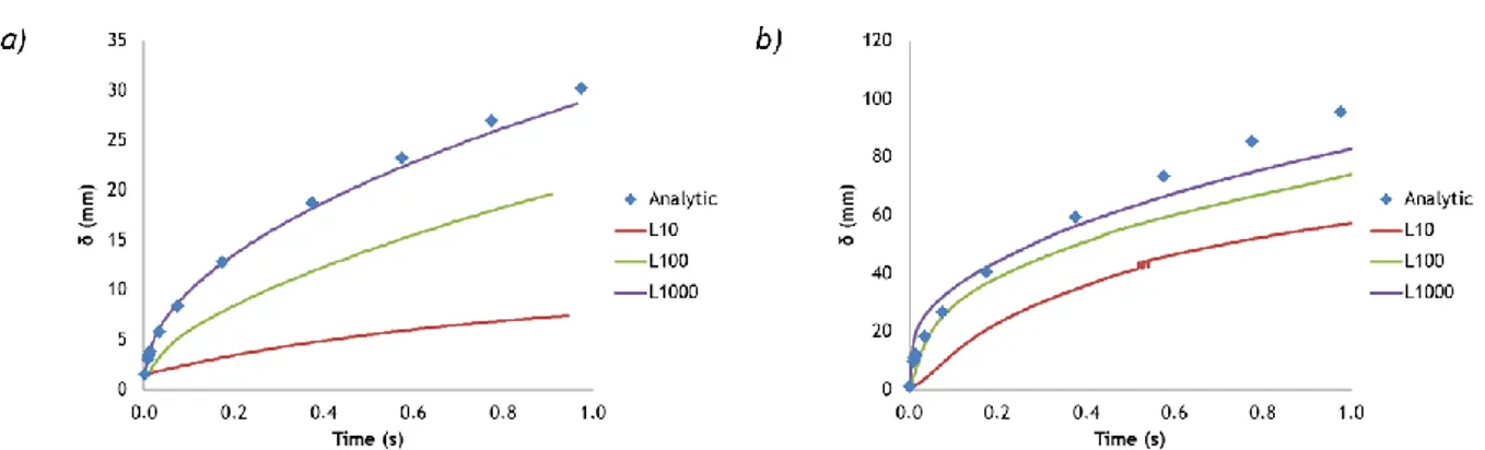
Following the position of the interface using an iso-surface (see Section 3.3.2) it is possible to obtain the distance to the heated wall and subsequently compare it to the analytic solution. The results of simulations for different Lee coefficients and and are illustrated in Figure 3. Note that the simulation runs in this sub-section do not include surface tension modeling.
Figure 3. Stefan Problem: Comparison between the analytic solution and CFD modeling (Lee Model) of the distance of the interface to the heated wall for different Lee coefficients and
Results and Discussion 19
From the above graphs, the effect of the Lee parameter clearly influences the movement of the interface displacement.
For and the simulation results can be considered an adequate fit to the analytical solution inside the timeframe considered of 1 second. A slight downward trend leads to the expectation of a deviation from the proper fit depicted in larger timeframes. For , the difference is more pronounced, failing to produce an accurate fit even for . From the lack of agreement between simulation and analytical solution for the Lee Coefficient in the interval considered it is possible to infer that the simulations making use of the Lee Model, as it is implemented, will not be able to produce accurate results. For higher Lee coefficients an approximation to the analytic solution is apparent for early time-steps; however a pervasive trend throughout the test is a relative slowing of the interface.
4.2.2 Surface Tension Modeling
The simulations previously considered did not model surface tension effects. Since it is reasonable to consider these effects could affect a gas-liquid interface, the test for
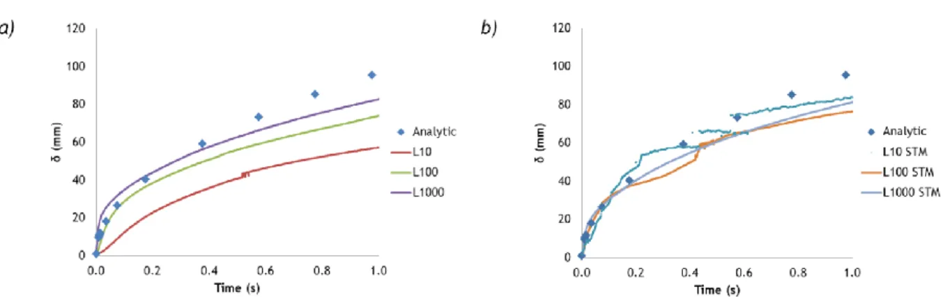
was repeated including surface tension modeling using the Continuum Surface Force model proposed by Brackbill and already implemented in ANSYS Fluent 16.0 (see Section 2.4). The result of this new simulation is illustrated in Figure 4 alongside the test for presented in Section 4.1.1.
Figure 4. Stefan Problem: Comparison between the analytic solution and CFD modeling (Lee Model) of the distance of the interface to the heated wall for different Lee coefficients and
a) no surface tension modeling and b) surface tension modeling and and
Results and Discussion 20
The inclusion of surface tension modeling significantly increases convergence issues, requiring manual adjustment of the time-step, and from Figure 4 it is evident an increase in noise effects, possibly numerical in origin, in the interface position measurement. Despite that, the new simulations produce results which are seemingly more accurante and precise, pointing to a dampening of the influence of the Lee coefficient.
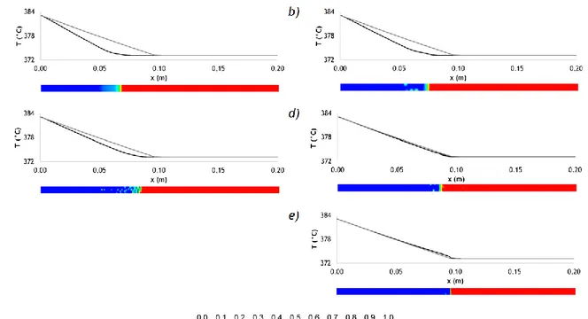
To better understand the behaviour of the interface it is helpful to look at the temperature profiles and volume fraction distribution across the domain at the end of the simulation ( ), pictured in Figure 5. Akin to Figure 4, the left column includes the simulations without surface tension modeling while the right column consists of the simulations with surface tension modeling.
Figure 5.Temperature profiles and volume fraction distribution at for a) and no STM; b) and STM; c) and no STM; d) and STM; e) and no
Results and Discussion 21
From Figure 5, it is possible to observe that the sharpness of the interface is kept for (Figure 5a and b); however uniformity in the direction parallel to the heated wall while maintaining said sharpness is observed only for and surface tension modeling (Figure 5b). The disparity between the expected temperature profile (analytic solution) and the one observed is in agreement with the difference in position observed between expected and observed (Figure 3 and Figure 4). A non-sharp interface, fractured like the ones evidenced in Figure 5c and Figure 5e or expanded like Figure 5d and Figure 5f, might interfere with the method used to measure (See Section 3.3). It is therefore necessary to evaluate the integrity of the interface through the temperature profiles and distribution of volume fractions in adition to the history of measurements to ascertain the quality of the adopted methods.
4.2.3 Conclusions
From the simulations using the Lee model it is possible to conclude that:
The adjustment parameter that characterizes this model (Lee coefficient) is shown to have an influence in the behaviour of the simulation;
Higher values of and lower values of produce the best fit to the analytic solution for the timeframe and conditions considered, while still evidencing some divergence to the analytic solution;
The inclusion of surface tension modeling results in increased convergence issues and computational time, although it helps reducing the influence of on the position of the interface;
Since the influence of the Lee coefficient was verified, finding an alternative model is preferred.
4.3 Non Parametric Model: Nichita Equation
The Nichita model was implemented in ANSYS Fluent using user-defined functions (UDF) since this model does not come already implemented in the commercial product’s source code. The addition of this model to ANSYS Fluent consists in four UDFs: one to define the temperature and volume fraction gradients and three to determine the mass and energy source terms (See Section 2.2). The code, written in C language, can be consulted in Appendix 1.
Results and Discussion 22 4.3.1 Mesh Sensibility Test
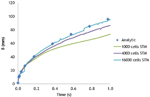
The first step in assessing the validity of the non-parametric model is to conduct a mesh sensibility test. Surface tension modeling, shown in Section 4.1 to produce slightly closer fits to the analytic solution, was included in the simulations. The test, as evidenced in Figure 6, produces a closer fit to the analytic solution. An unexpected result is the emergence of an effect analog to numerical noise for more refined meshes.
Figure 6. Comparison between the analytic solution and CFD modeling (Nichita Model) of the distance of the interface to the heated wall for different mesh refinements. For all runs
and .
The increasingly better fit for more refined meshes points towards using highly refined meshes as a solution to the deviations in observed; however along with the improved results so did the calculation time increase considerably, even when running in a dedicated cluster computer: quadrupling the cell count results in a considerable increase in computation time (from 37 for up to 55 h for ).
4.3.2 Surface Tension Modeling
Given the increased computation time when modeling the surface tension, it is worth reconsidering its inclusion in the test for this new model. Comparative tests for different mesh densities (1000 and 4000 cells) were run to reassess the effect of STM. The measured distance to the heated wall ( ) for the different cases is compared to the analytic solution to the Stefan Problem in Figure 7 .
Results and Discussion 23
Figure 7. Comparison between the analytic solution and CFD modeling (Nichita Model) of the distance of the interface to the heated wall with and without STM for a) and b)
.
From the results it is possible to infer the positive influence of modeling surface tension forces in both noise cancelling and closeness to the analytic solution. The increased computational time and number of convergence issues when including STM observed for the Lee model are also verified for the Nichita model. The temperature profiles and volume fraction distribution for different degrees of mesh refinement and inclusion/exclusion of surface tension modeling are represented in Figure 8.
Figure 8. Temperature profiles and volume fraction distribution at for a)
and no STM; b) and STM; c) and no STM; d) and
Results and Discussion 24
Analyzing the volume fraction distribution at , evidence of artifacts in the form of pockets of G/L mixture in the vapour phase are present in simulations 6b to e. Looking at the simulations without STM, the one where has expanded while the one where has fragmented into several pockets of mixture. The simulations with surface
tension modeling seem to remain intact to some extent, with the thickness of the interface being inversely proportional to the mesh refinement. The proximity of the simulated and teoric temperature profiles coincide with the accuracy of the measurement in Figure 6; however the sharpness of the interface is unexpected giving the pronounced numerical noise-like effect found for Looking at the volume fraction distribution for time-steps just before and after it becomes evident that the behaviour of the interface is much more irregular than suggested in Figure 8. Details of the interface for time-steps just before and after are depicted in Figure 9.
Figure 9. Detail of the volume fraction distribution for the test with and STM
at a) , b) , c) .
4.3.3 Conclusions
Using the Nichita model model:
Refining the simulation domain produces closer fits to the analytic solution at the cost increased computational times and irregularities in the interface;
Modeling surface tension helps maintaining the integrity of the interface and provides a better fit to the analytic solution, however increases computational time significantly;
From the volume fraction profiles, evidence of G/L mixture artifacts can be found away from the interface, which is possibly related to the numerical noise effect perceived while measuring
Results and Discussion 25
4.4 Non Parametric Model: Sun Equation
The Sun model is also absent from the ANSYS Fluent library. Due to its similarity to the Nichita model, its implementation is similar to the one described in Section 4.3, only differing in the equations that characterize the source terms. The code for the Sun model can also be found in Appendix 1.
The simulations in this section, taking into account the conclusions from the Nichita model simulations, have been performed for the mesh with and include surface tension modeling with .
4.4.1
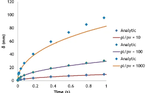
Behaviour for differentThe distance to the heated wall for different using the Sun Model and its comparison to the analytic solution to the Stefan Problem is illustrated in Figure 10.
Figure 10. Comparison between the analytic solution and CFD modeling (Sun Model) of the distance of the interface to the heated wall for different . and
.
From the results it is possible to recognize a good agreement between simulations and analytic solution for lower however the current model does not describe the analytic results for the full range of in study. The discrepancy between measured and the analytic solution for is a trend that is expected to occur for lower provided a larger timeframe is considered.
Results and Discussion 26
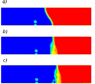
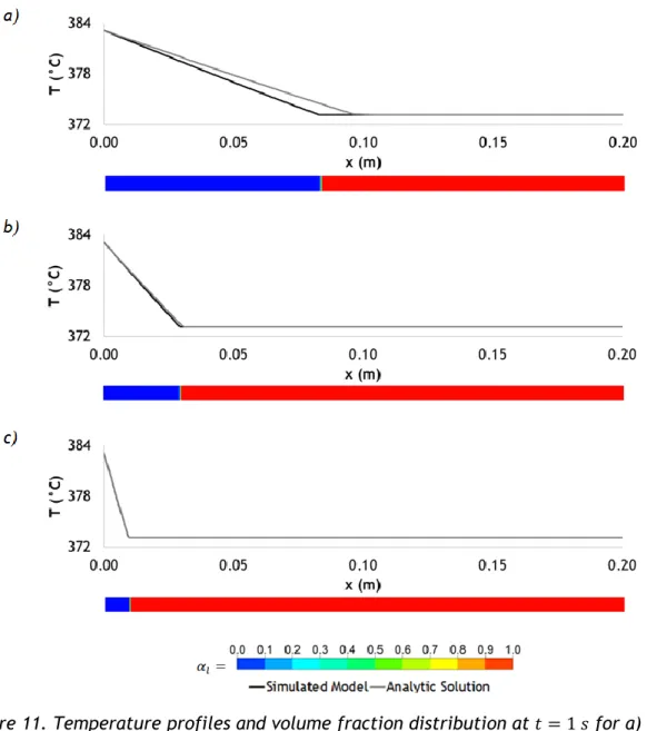
Analyzing the volume fraction distribution at , depicted in Figure 11, it is noticeable that there is no interface expansion or deformation, no artifacts are produced and the temperature profile displays a sharp behaviour. For higher however, the interface does not move in tandem with the analytical solution.
Figure 11. Temperature profiles and volume fraction distribution at for a)
Results and Discussion 27 4.4.2 Conclusions
Regarding the Sun Model:
For the time domain considered, this model shows a good fit between simulation and analytic results for and lower;
The trend observed for the simulation results lead to the belief that the Sun model will not accuse a good fit if higher timeframes are taken into consideration;
The temperature and volume fraction profiles show a significantly sharper and intact interface compared to the previous two models;
For the abovementioned reasons, regarding the fluids and timeframes considered the Sun model outperforms both the Lee and Nichita models for boiling flows.
References 28
5 Conclusion
5.1 Accomplishments
This work has consisted in a comparative test between three different phase change models using the Stefan Problem as a benchmark: the Lee model, the Nichita model and the Sun model. The case study also tested the influence of elements such as surface tension modeling (through the Continuum Surface Force model), mesh density and different .
The tests done on the Lee Model have confirmed a dependence on an adjustable parameter . Inclusion of surface tension modeling resulted in increased convergence issues, however reducing the influence of the Lee coefficient in terms of position of the interface. This dependence is undesireable, therefore alternative models are preferred.
The tests on the Nichita Model have shown refining the domain produces simulations closer to the analytic solution, at the cost of increased computational times. From the volume fraction profiles, evidence of G/L mixture artifacts can be found away from the interface. Modeling surface tension helps maintaining the integrity of the interface and provides a better fit to the analytic solution, at the cost of increased computational time.
The temperature and volume fraction profiles for the Sun Model show a significantly better preserved interface compared to the previous two models. For the time domain considered, the model shows a good fit between simulation and analytic results for and lower. However, the trend of the results for lead to the belief that the Sun model will not accuse a good fit if higher timeframes are taken into consideration.
This case study, while not resulting in a reliable model for phase-changing flows in industrial settings, provides valuable information on the reliability of existing methods using source terms. This information is expected to be useful for future assessments and influence future work for the development of such a tool.
5.2 Limitations of this work
Higher cell densities become particularly hard to solve in acceptable timeframes;
The non parametric methods, as currently implemented, do not take into account the fluid’s saturation temperature;
The chosen fluid has no direct functional analog in the real world;
References 29
5.3 Future Work
There are several aspects to consider for future work that can be divided in two categories: improvement of current models and additional testing steps.
As a way of possibly improving the current models, include in the UDF code accounting for the boiling point of the fluid being tested, testing the models with a different front-capturing method such as the Level-Set Method and study the possibility of applying Dynamic Meshing as a way of reducing the computational burden of the simulations.
Additional testing steps include substituting the fluid used in this work for ones with industrial significance (such as water and heptanes) as well as identify and implement benchmarks in two and three dimensions (bubble growth and departure on a heated plate, experiments on pilot plant tubing).
5.4 Final Thoughts
The work has proven to be interesting, challenging and very open-ended. As such, the possibility for continuation is immense, where the author encourages both refining the existing results and pursuing alternative routes in the hopes of reaching the ultimate goal put forth by IFPEN.
References 30
6 References
ANSYS Inc, 2015. ANSYS Fluent Theory Guide.
Brackbill, J., Kothe, D., Zemach, C., 1991. A Continuum Method for Modeling Surface Tension. Journal of Computational Physics 100, 335-354.
Dhir, V., Son, G., 1998. Numerical simulation of film boiling near critical pressures with a level set method.Journal of Heat Transfer 120, 183-192.
Nichita, B., Thome, J., 2010. A level set method and a heat transfer model implemented into FLUENT for modeling of microscale two phase flows. Journal of Fluids Engineering 132 (8).
Sun, D., Xu, J., Wang, L., 2012. Development of a vapor-liquid phase change model for volume-of-fluid method in FLUENT. International Communications in Heat and Mass Transfer 39, 1101-1106.
Tryggvason, G., Scardovelli, R., Zaleski,S., 2011. Direct Numerical Simulations of Gas-Liquid Multiphase Flows. Cambridge University Press.
Welch, S., Wilson, J., 2000. A volume of fluid based method for fluid flows with phase change. Journal of Computational Physics 160, 662-682.
Appendixes 31
7 Appendixes
7.1 User Defined Functions
7.1.1 Nichita Model #include "udf.h" #include "sg_mphase.h" #include "mem.h" #include "sg_mem.h" #include "sg_vof.h" #include "flow.h" #define latheat 10000 DEFINE_ADJUST(allocate_vof,domain) { Thread *thread; Thread **phase_th; cell_t cell;
Domain *pDomain = DOMAIN_SUB_DOMAIN(domain,P_PHASE); #if !RP_HOST Alloc_Storage_Vars(pDomain,SV_VOF_RG,SV_VOF_G,SV_NULL); Scalar_Reconstruction(pDomain, SV_VOF,-1,SV_VOF_RG,NULL); Scalar_Derivatives(pDomain,SV_VOF,-1,SV_VOF_G,SV_VOF_RG,Vof_Deriv_Accumulate); Alloc_Storage_Vars(domain, SV_T_RG, SV_T_G, SV_NULL); T_derivatives(domain); #endif mp_thread_loop_c(thread,domain,phase_th) { if (FLUID_THREAD_P(thread))
Appendixes 32
{
Thread *pri_th = phase_th[P_PHASE]; begin_c_loop (cell,thread) { #if RP_3D C_UDMI(cell,thread,0) = -(C_VOF_G(cell,pri_th)[0]*C_T_G(cell,thread)[0]+C_VOF_G(cell,pri_th)[1]*C_T_G(cell,thread)[ 1]+C_VOF_G(cell,pri_th)[2]*C_T_G(cell,thread)[2]); C_UDMI(cell,thread,4) = -C_VOF_G(cell,pri_th)[0]; C_UDMI(cell,thread,5) = -C_T_G(cell,thread)[0]; #endif #if RP_2D C_UDMI(cell,thread,0) = -(C_VOF_G(cell,pri_th)[0]*C_T_G(cell,thread)[0]+C_VOF_G(cell,pri_th)[1]*C_T_G(cell,thread)[ 1]); C_UDMI(cell,thread,4) = -C_VOF_G(cell,pri_th)[0]; C_UDMI(cell,thread,5) = -C_T_G(cell,thread)[0]; #endif } end_c_loop(cell,thread) } } }
/* Hooked as a mass source in liquid domain */ DEFINE_SOURCE(liq_src, cell, pri_th, dS, eqn) {
Thread *mix_th, *sec_th; real source_l;
/* SI Units */
real lat_heat = latheat;
mix_th = THREAD_SUPER_THREAD(pri_th); sec_th = THREAD_SUB_THREAD(mix_th,1);
Appendixes 33 source_l = -(C_VOF(cell,pri_th)*C_K_L(cell,pri_th)+C_VOF(cell,sec_th)*C_K_L(cell,sec_th))*C_UDMI(cell,m ix_th,0)/lat_heat; dS[eqn] = 0.0; C_UDMI(cell,mix_th,2)= source_l; return source_l; }
/* Hooked as a mass source in gas domain */ DEFINE_SOURCE(vap_src, cell, sec_th, dS, eqn) {
Thread *mix_th, *pri_th; real source_v;
/* SI Units */
real lat_heat = latheat;
mix_th = THREAD_SUPER_THREAD(sec_th); pri_th = THREAD_SUB_THREAD(mix_th,0); source_v = (C_VOF(cell,pri_th)*C_K_L(cell,pri_th)+C_VOF(cell,sec_th)*C_K_L(cell,sec_th))*C_UDMI(cell,m ix_th,0)/lat_heat; dS[eqn] = 0.0; C_UDMI(cell,mix_th,1)= source_v; return source_v; }
/* Hooked as an energy source in mixture domain */ DEFINE_SOURCE(enrg_src, cell, mix_th, dS, eqn) {
Thread *pri_th, *sec_th; real source_e;
Appendixes 34 pri_th = THREAD_SUB_THREAD(mix_th,0); sec_th = THREAD_SUB_THREAD(mix_th,1); source_e = (C_VOF(cell,pri_th)*C_K_L(cell,pri_th)+C_VOF(cell,sec_th)*C_K_L(cell,sec_th))*C_UDMI(cell,m ix_th,0); dS[eqn] = 0.0; C_UDMI(cell,mix_th,3)= source_e; return source_e; }
Appendixes 35 7.1.2 Sun Model #include "udf.h" #include "sg_mphase.h" #include "mem.h" #include "sg_mem.h" #include "sg_vof.h" #include "flow.h" #define latheat 10000 DEFINE_ADJUST(allocate_vof,domain) { Thread *thread; Thread **phase_th; cell_t cell;
Domain *pDomain = DOMAIN_SUB_DOMAIN(domain,P_PHASE); #if !RP_HOST Alloc_Storage_Vars(pDomain,SV_VOF_RG,SV_VOF_G,SV_NULL); Scalar_Reconstruction(pDomain, SV_VOF,-1,SV_VOF_RG,NULL); Scalar_Derivatives(pDomain,SV_VOF,-1,SV_VOF_G,SV_VOF_RG,Vof_Deriv_Accumulate); Alloc_Storage_Vars(domain, SV_T_RG, SV_T_G, SV_NULL); T_derivatives(domain); #endif mp_thread_loop_c(thread,domain,phase_th) { if (FLUID_THREAD_P(thread)) {
Thread *pri_th = phase_th[P_PHASE]; begin_c_loop (cell,thread)
Appendixes 36 { #if RP_3D C_UDMI(cell,thread,0) = -(C_VOF_G(cell,pri_th)[0]*C_T_G(cell,thread)[0]+C_VOF_G(cell,pri_th)[1]*C_T_G(cell,thread)[ 1]+C_VOF_G(cell,pri_th)[2]*C_T_G(cell,thread)[2]); #endif #if RP_2D C_UDMI(cell,thread,0) = -(C_VOF_G(cell,pri_th)[0]*C_T_G(cell,thread)[0]+C_VOF_G(cell,pri_th)[1]*C_T_G(cell,thread)[ 1]); #endif } end_c_loop(cell,thread) } } }
/* Hooked as a mass source in liquid domain */ DEFINE_SOURCE(liq_src, cell, pri_th, dS, eqn) {
Thread *mix_th, *sec_th; real source_l;
/* SI Units */
real lat_heat = latheat;
mix_th = THREAD_SUPER_THREAD(pri_th); sec_th = THREAD_SUB_THREAD(mix_th,1); if (C_T(cell,sec_th)>373.15) source_l = -(2*C_K_L(cell,sec_th)*C_UDMI(cell,mix_th,0))/lat_heat; else source_l = 0.; dS[eqn] = 0.0; C_UDMI(cell,mix_th,2)= source_l;
Appendixes 37
return source_l; }
/* Hooked as a mass source in gas domain */ DEFINE_SOURCE(vap_src, cell, sec_th, dS, eqn) {
Thread *mix_th, *pri_th; real source_v;
/* SI Units */
real lat_heat = latheat;
mix_th = THREAD_SUPER_THREAD(sec_th); pri_th = THREAD_SUB_THREAD(mix_th,0); if (C_T(cell,sec_th)>373.15) source_v = (2*C_K_L(cell,sec_th)*C_UDMI(cell,mix_th,0))/lat_heat; else source_v = 0; dS[eqn] = 0.0; C_UDMI(cell,mix_th,1)=source_v; return source_v; }
/* Hooked as an energy source in mixture domain */ DEFINE_SOURCE(enrg_src, cell, mix_th, dS, eqn) {
Thread *pri_th, *sec_th; real source_e;
pri_th = THREAD_SUB_THREAD(mix_th,0); sec_th = THREAD_SUB_THREAD(mix_th,1); if (C_T(cell,sec_th)>373.15)
Appendixes 38 source_e = -2*C_K_L(cell,sec_th)*C_UDMI(cell,mix_th,0); else source_e = 0; dS[eqn] = 0.0; C_UDMI(cell,mix_th,3)= source_e; return source_e; }
Appendixes 39
7.2 Mesh Illustrations
Appendixes 40 7.2.2 4000 Cells
Appendixes 41 7.2.3 16000 Cells