EFFICIENT SCREENING OF VARIABLE SUBSETS IN MULTIVARIATE STATISTICAL MODELS
A. Pedro Duarte Silva
Faculdade de Ciências Económicas e Empresariais,
Universidade Católica Portuguesa - Centro Regional do Porto Rua Diogo Botelho, 1327
4150 PORTO PORTUGAL Email: [email protected]
In applied statistical studies, it is common to collect data on a large pool of candidate variables from which a small subset will be selected for further analysis. The practice of variable selection often combines the use of substantive knowledge with subjective judgment and data-based selection procedures. The most popular of such procedures are stepwise methods. However, stepwise selection methods have two fundamental shortcomings:
a) Most theoretical results from classical statistics require the assumption that the set of variables to be analyzed was chosen independently of the data. Therefore, when the variables are selected based on the data, the results from classical distribution theory almost never hold.
b) Stepwise selection methods look at one variable at a time and tend to ignore the impact of combining particular sets of variables together. Thus, as each variable “importance” is often influenced by the set variables currently under analysis, stepwise methods may fail to identify the most adequate variable subsets.
The problems created by a) and b) are now widely recognized and have been discussed by several authors. Miller (1984, 1990) and Derksen and Keselman (1992) give good reviews of the relevant literature in the context of Regression Analysis. In the context of Discriminant Analysis the problems created by a) are discussed, among others, by Murray (1977), McKay and Campbel (1982a), Snapinn and Knoke (1989) and Turlot (1990), and the problems created by b) are discussed by Hand (1981), McKay and Campbel (1982a, 1982b) and Huberty and Wisenbaker (1992).
The problem referred in b) can be overcome by procedures that compare all possible variable subsets according to appropriate criteria. However, this approach usually requires the evaluation of a large number of alternative subsets, and may not be feasible. For regression models, several efficient algorithms were developed in order to surpass this problem. For instance, for the linear regression model with p candidate variables, Beale, Kendall and Mann (1967) and Hocking and Leslie (1967) proposed branch and bound algorithms that identify “the best” (in the sense of R2) variable subsets, evaluating only a small fraction of the 2p-1 different subsets. Furnival (1971) has shown how the residual sum of squares for all possible regressions can be computed with an effort of about six floating point operations per regression. Furnival and Wilson (1974) combined Furnival algorithm with a branch and bound procedure, leading to the widely used “leaps and bounds” algorithm for variable
selection. Lawless and Singhal (1978) adapted Furnival and Wilson algorithm to non-linear regression and Kuk (1984) applied the former adaptation to proportional hazard models in survival analysis.
This article will focus on efficient algorithms for all-subsets comparisons in multivariate analysis. In particular, it will be shown how Furnival and Wilson “leaps and bounds” can be adapted to compare, according to appropriate criteria, variable subsets in Discriminant Analysis, MANOVA, MANCOVA, and Canonical Correlation Analysis. To the best of our knowledge, algorithms to surpass the difficulties created by b) have not received the same amount of attention in multivariate models as in regression. Some exceptions include the following research. McCabe (1975) adapted Furnival’s algorithm to the comparison (accord-ing to Wilk’s Λ) of variable subsets in Discriminant Analysis. McHenry (1978) proposed a compromise between stepwise and all-subsets procedures in multivariate linear models. Seber (1984, pp 507-510) discusses extensions of McCabe approach to variable comparisons concerning linear hypothesis in multivariate models, and briefly mentions that branch and bound algorithms can also be employed. Duarte Silva (forthcoming) adapted Furnival and Wilson “leaps and bounds” to the minimization of parametric estimates of the error rate in two-group Discriminant Analysis.
No attempt will be made here to deal with the difficulties referred in a). Although any data-based variable selection procedure usually leads to violations of the assumptions underlying classical inference methods, that should be no reason for ignoring the data in the variable selection process. Anyway, for the purpose of statistical inference it is not recommended that the effects of variable selection should be ignored. When inference is required and the variables are not chosen a-priori, specialized procedures should be employed. Some possibilities in that regard, include the use of cross-validation techniques, like bootstrap methodologies that explicitly take into account the selection process (ex: Snapinn and Knoke 1989).
All the procedures discussed in this article are being programmed in the C++ language. A public-domain software implementation for Personal Computers can be ordered directly from the author and will soon be available on the internet at the address http://www.porto.ucp.pt/~psilva.
OUTLINE OF “LEAPS AND BOUNDS” ALGORITHMS
Most modern algorithms for all-subsets comparisons in statistical models are based on adaptations of Furnival (1971) and Furnival and Wilson (1974) algorithms for variable selection in linear regression. Within a general framework, these algorithms may be outlined as follows. Assume that there are p candidate variables, X1, X2, ..., Xp to enter a given
statistical model. Denote the different subsets of {X1, X2, ..., Xp} by S1, S2, ..., S2P-1, where
S1 = X represents the full set comprising all p candidates. We are interested in the
compari-son of S1, S2, ..., S2P-1, according to appropriate criteria of “model quality”. Suppose that it
is possible to define one such criterion, C(Sa), that can be expressed as a function of a
quadratic form, Q(Sa), with general expression Q(Sa) = vSa’ MS S . -1
a a vSa
The following notation is adopted through this text. Matrices are denoted by bold upper case and vectors by bold lower case. Individual elements of vectors and matrices are denoted by lower case subscripts. The portions of vectors and matrices associated with the variables included in a given subset, Sa, are denoted by the subscripts Sa (vectors) and SaSa (matrices).
The complement of Sa is denoted by Sa and the matrices comprised by the rows (columns)
associate with variables included in Sa and columns (rows) associated with variables
excluded from Sa are denoted by the subscripts SaSa ( SaSa). The i-th row (j-th column) of a
matrix associated with the variables included in Sa is denoted by the subscripts i,Sa (Sa,j).
Assume that there are a column vector and a symmetric matrix M satisfying the following conditions:
vS1 S S1 1
(A) The (i,j) element of MS S , M
1 1 ij, is a function of the values of Xi and Xj. Mij is not
influenced by any variable other than Xi and Xj.
(B) The i-th element of vS , v
1 i, is a function of the values of Xi. vi is not influenced
by any variable other than Xi.
Then, Furnival algorithm is essentially a method for evaluating all forms Q(Sa) with minimal
computational effort. In the linear regression model y = Xβ + u,
a natural comparison criterion is the Residual Sum of Squares, = y’ y which can be evaluated by choosing M and respectively as the matrix of Sums of Squares and Cross Products (SSCP) among the regressors and vector of sums of crossproducts between the regressors and the dependent variable, i.e., = X’X and = X’ y. In that case C
RSSSa y ' X ) X ' (X X y' a a a a S 1 S S S − S S1 1 vS1 MS S(1) 1 1 vS(1) 1 (1)
(Sa) = RSSSa = y’ y - Q(1)(Sa). However, in most
implementations of the algorithm, for reasons of numerical stability, these sums are replaced by correlations, defining MS S and instead as = R
1 1 vS1 MS S
(2)
1 1 XX , vS = r
(2)
1 Xy. This choice leads
to the equivalent criterion C(2)(Sa) = RS2a = rX y RX X r = Q 1
X y
Sa ' Sa Sa Sa
− (2)
(Sa).
The fundamental mechanics of the algorithm are as follows. Initially, create the source matrix MV(Ø), associated with the empty subset, whereMS S and should satisfy (A) and (B).
1 1 vS1 MV(Ø) = M v (1) v S S S S ' 1 1 1 1 0 ⎡ ⎣ ⎢ ⎤ ⎦ ⎥
Next, start “bringing variables into the model” by performing specialized Gauss-Jordan elimination operations known as “symmetric sweeps” (Beale, Kendall and Mann 1967). After “sweeping” all the elements of Sa, MV(Ø) is converted into matrix MV(Sa), where,
without lack of generality, it is assumed that the rows and columns associated with Sa are
placed before those associated with Sa.
MV(Sa) = − − − − − − − − − ⎡ ⎣ ⎢ ⎢ ⎢ ⎤ ⎦ ⎥ ⎥ ⎥ − − − − − − − − M M M M v M M M M M M v M M v v ' M v v ' M M v ' M v S S 1 S S 1 S S S S 1 S S S S S 1 S S S S S S 1 S S S S S S S 1 S S S S 1 S S S S 1 S S S S S 1 S a a a a a a a a a a a a a a a a a a a a a a a a a a a a a a a' a a a a a a a a a − (2)
As Q(Sa) = -1*MV(Sa)p+1,p+1 the comparison criterion C(Sa) can be updated after each sweep.
A symmetric sweep on variable Xk ∈ Sa, uses equations (3) through (5) to convert MV(Sa)
into MV(Sb) with Sb = Sa ∪ {Xk}.
MV(Sb)kk = -1 / MV(Sa)kk (3)
MV(Sb)kj = MV(Sb)jk = MV(Sb)kk * MV(Sa)kj (j ≠ k) (4)
MV(Sb)ij = MV(Sb)ji = MV(Sa)ij + MV(Sb)kj * MV(Sa)ik (i ≠ k, j ≠ k) (5)
Furnival minimizes computational effort by taking advantage of the following facts. As the symmetry of the matrices MV(.) is always preserved, only elements on or above their diagonals need to be stored and updated. Furthermore, MV(Sb)p+1,p+1 = MV(Sa)p+1,p+1 -
and each update of Q(S
MV(S )a 2k,p+1/MV(S ) a kk a) requires only two floating point
opera-tions (multiplicaopera-tions and divisions). When MV(Sb) is not used to evaluate other subsets, all
its remaining elements can be ignored. When MV(Sb) is used to evaluate other subsets
involving at most t additional variables, then the elements associated with these variables also need to be updated. In that case, a sweep requires (t+1)*(t+4)/2 floating point operations. By ordering the evaluation of subsets in a appropriate manner it is possible to evaluate all forms
Q(Sa) is such a way that: (i) The value of each Q(Sb), can be derived from a sub-matrix of
MV(Sa), where Sa has exactly one less variable than Sb. (ii) Only p (portions of) matrices
MV(.) need to be kept simultaneously in memory. (iii) The number of different sub-matrices that are used in the evaluation of subsets with (at most) t additional variables (t=0,1,...,p-1) equals 2p-t-1.
A remarkable consequence of (iii), is that a full (p+1)*(p+1) matrix sweep never needs to be performed, a p*p sweep needs to be performed only once, a (p-1)*(p-1) sweep twice, and (following the same pattern) approximately half (more precisely 2p-1) of the MV(.) matrices are not used in the evaluation of additional subsets. Furnival and Wilson (1974) show that the total number of floating point operations used in Furnival algorithm equals 6(2p) - p(p+7)/2 - 6, and that it is not possible to compute all Q(Sa) with fewer operations.
McCabe (1975) has shown that Furnival algorithm can be adapted to evaluate criteria based on determinants. In particular, if M is a matrix satisfying condition (A), then all determi-nants | | can be computed using the following algorithm. Create the initial matrix MD(Ø) = . Initialize the auxiliary variable D(Ø) = 1. Proceed as in the original algorithm, and each time MD(S
S S1 1
MS S
a a
MS S
1 1
a) is updated to MD(Sb) by sweeping on Xk , also compute D(Sb) = D (Sa) * MD(Sa)kk.
As |MS S | = | M | * (M
b b S Sa a kk - M ) it follows that this procedure will ensure
that D (S k,Sa MS S 1 a a − MS ,k a
a) = |MS Sa a| for all non-empty subsets Sa. The adaptation described above was used
by McCabe to compare variable subsets in Discriminant Analysis and, as it will be discussed in the following sections, has wide applicability in several multivariate models.
Although when it is desired to evaluate all alternative subsets, it is not possible to improve upon the efficiency of Furnival’s algorithm, in practice often it is only required the identifica-tion of “good” subsets for further inspecidentifica-tion. In order to select the best variable subsets according to a given criterion, it is possible to employ search procedures that are able to recognize that many subsets will never be selected before evaluating them. That is the philosophy behind “branch and bound” algorithms for variable selection. Maybe the best known of these algorithms is the “leaps and bounds” algorithm of Furnival and Wilson for
linear regression. Furnival and Wilson algorithm is based on the following properties: (i) The Residual Sum of Squares of a given model can never decrease with the removal of variables, i.e., Sa ⊂ Sb ⇒
RSSS
a ≤ . ii) Symmetric sweeping is reversible. In effect, if the elements of MV(.) are multiplied by minus one, then the symmetric sweep operator updates the resulting matrices when variables are removed. Creating initially the matrices MV(Ø) and MV(S
RSSS
b
1)
associated respectively with the empty and full subsets, Furnival and Wilson build a search tree that on the left side moves from MV(Ø) adding variables to previous subsets and on the right side moves from MV(S1) removing variables. Finding on the left side of the search tree
“good” subsets early on, it is often possible to prune large branches of the search tree that given (i) can never include subsets “deserving” to be selected. In their original article, Furnival and Wilson describe some “smart” strategies to conduct the search, that attempt to maximize pruning, while ensuring that in the worst case (no pruning) the number of floating point operations approaches six per subset.
The basic ideas behind Furnival and Wilson algorithm are not restricted to linear regression models. In fact, they can be applied in any model where it is possible to define criteria that never improve with the removal of variables and operators to reevaluate these criteria upon the addition or removal of single variables. The computational efficiency of such procedures is bound to be dependent on the effort required by these operators. For criteria derived from quadratic forms based on matrices and vectors satisfying (A) and (B), Furnival strategy can be used and the reevaluation of the appropriate criteria is computationally “cheap”. The same applies to criteria derived from determinants based on matrices satisfying (A), because the operator used in McCabe’s adaptation of Furnival algorithm is also reversible, i.e., if
D (Sb) = |MS Sb b|, then D (Sa) = D (Sb) * MD(Sb)kk = | MS Sa a | (with Sb = Sa ∪ {Xk}). This
property can be easily derived from standard results on the determinants and inverses of partitioned matrices. Criteria not based on quadratic forms or determinants usually lead to computational difficulties that rend all-subset comparison procedures unfeasible for a moderate number of candidate variables.
VARIABLE SCREENING IN TWO-GROUP DISCRIMINANT ANALYSIS
Discriminant Analysis (DA) studies can have two major objectives: (i) Interpreting and describing group differences. (ii) Allocating entities to well-defined groups, based on a relevant set of entity attributes.
Techniques dealing with problems of the first type of are usually headed under the designa-tion of descriptive DA, and methods dealing with problems of the second type have been called predictive DA, allocation or classification methods. However, the word classification is also used to designate Cluster Analysis methodologies and the expression predictive DA, may refer to Bayesian approaches to allocation problems (McLachlan 1992, pp 67-74). Therefore, in order to avoid unnecessary confusions, the term allocation will be adopted in this article. Descriptive DA techniques can also be used to interpret significant effects found by a multi-factor MANOVA or MANCOVA (Kobilinsky 1990, Masson 1990, Huberty 1994 pp 206). In this and the following sections, a more traditional view will be adopted, assum-ing that every group can be defined by the level of a sassum-ingle factor in a MANOVA model. The choice of criteria to compare variable subsets in DA should pay particular attention to the objectives of the analysis. In particular, several methodologists (McKay and Campbel
]
1982a, 1982b, Huberty 1994) recommend that in descriptive studies, variables should be compared based on measures of group separation, while in allocation studies it is more appropriate to use estimates of prediction power. However, in two-group problems both approaches can lead to similar procedures. Consider the traditional approach to two-group allocation, based on the assumptions of multivariate normality and common within-groups variance-covariance matrix ∑. In that case, it is well known the optimal hit rate is a decreas-ing function of the Mahalanobis distance between group means, ∆ =
[
(µ1−µ2) 'Σ−1(µ1−µ2) 1 2/ (where µ1 and µ2 denote the means of groups 1 and 2). In adescriptive context, the most usual index of group separation is the sample analogue of ∆,
[
]
D= (x1−x2)'S−1(x −x ) /
1 2
1 2
(where x1,x2 and S are the sample mean vectors and sample pooled variance-covariance matrix). In allocation problems, D is also a reasonable criterion for subset comparisons, as several estimators of hit rates are based on it. For instance, assuming equal prior probabilities of group membership, Fisher proposed Φ(D/2) (Φ(.) being the cumulative probability of a standard normal variate) as an estimator for the actual hit rate of the classical allocation scheme, based on the Linear Discriminant Function (Fisher 1936). Although Φ(D/2) is optimistically biased, several authors (Lachenbruch 1968, Lachenbruch and Mickey 1968, McLachlan 1974) derived bias-correction factors, leading to parametric estimators that, once the sample dimension and number of variables are fixed, are simple functions of D.
The adaptation of Furnival algorithm to the comparisons of variable subsets based on D is straightforward. Following the notation of previous section, ifvS and are chosen as
1 MS S1 1
x1−x2 and S, then the conditions (A)-(B) are satisfied and Q(Sa) = DS2a. Furthermore, D
2
never increases with the removal of variables, and the “leaps and bounds” approach of Furnival and Wilson can also be employed. Duarte Silva (forthcom-ing) has implemented this approach, using McLachlan’s estimate of the hit rate (McLachlan 1974) as comparison criterion, C(Sa). With the help of a personal computer, for several
problems with 30 candidate variables, Duarte Silva was always able to identify to 20 best subsets according to C(Sa) in less than 20 minutes of CPU time.
A potential drawback of the approach described above, is the fact that this approach is based on parametric estimators of hit rates, which relay on fairly strong assumptions and are not particularly robust (McLachlan 1986). Furthermore, there are many non-parametric estima-tors of hit rates that have good properties under a wide range of data conditions (McLachlan 1992, pp 337-366). These estimators typically require some “counting scheme” associated with a cross-validation strategy (ex: jackknife, leave-one-out or bootstrap) to avoid optimistic bias. As non-parametric estimates of hit rates are not based on quadratic forms or determi-nants, Furnival algorithm can not be easily adapted to their repeated computation.
Thus, the choice of criteria for subsets comparisons in allocation problems, may require evaluating a trade-off between stepwise procedures based on criteria (non-parametric estimates) with good properties for a wide range of data conditions, and all-subsets proce-dures based on criteria (parametric estimates) whose quality can only be guaranteed for specific conditions. A rigorous and complete analysis of this trade-off is beyond the scope of this article. However, given the article emphasis on all-subset comparisons as an alternative to stepwise procedures, an effort will be made in order to identify and characterize data conditions where the problems of stepwise methods are more pronounced.
Consider a two-group discriminant problem where the traditional assumptions of multivariate normality and equality of variance-covariances hold. Then, as discussed above, the popula-tion Mahalanobis distance associate with a subset Sa ( ) is an appropriate measure of the
S
a
S
∆
a “quality” both for descriptive and allocation purposes. Thus, when an additional variable,
Xk (Xk ∈ Sa) , is added to Sa leading to subset Sb, the contribution of Xk can be interpreted
in terms of the increase in squared Mahalanobis distance, - . Using expressions (2)-(5). it follows that the increase in a quadratic form Q(S
∆S b
2 ∆
Sa
2
a) upon the addition of Xk is given by:
Q(Sb) - Q(Sa) = (v M M v ) M M M M k k,S S S 1 S 2 kk k,S S S 1 S ,k a a a a a a a a − − − − (6)
In particular, makingvS1 = (µ1 - µ2) and MS S1 1 = ∑, the increase in ∆
2 is given by: ∆S b 2 -∆S = a 2
[
]
k S S S S k kk S S S S S k k k a a a a a a a a a , 1 , 2 2 1 1 , 2 1 ) ( ) ( Σ Σ Σ Σ µ µ Σ Σ µ µ − − − − − − (7)Formula (7) deserves close attention. It is known, from the properties of the multivariate normal distribution, that E(Xk|Sa) = α + βXSawith β = . Thus, the numerator of (7) can be expressed as . Therefore, the contribution of X
1 , − a a a SS S k Σ Σ
[
2 2 1 2 1 ) ( ) ( a a S S k k µ β µ µ µ − − −]
k to thegroup separation (as measured by ∆2
) is not directly related to its average difference across groups, µ −1k µ2k, but to the difference between µ −1k µ2k and β(µ1Sa −µ2Sa). This latter
value can be interpreted as the across-group mean difference of Xk, explained by the relation
between Xk and the elements of Sa. The denominator of (7) can be expressed alternatively as
, where denotes the variance of X σXk ρXk S
2 2
1
( − . a ) σXk
2
k and the squared correlation
between X
ρXk.Sa
2
k and Sa. Thus, the denominator of (7) equals the conditional variance of Xk given
Sa, and the contribution of Xk to ∆2, is simply the ratio between the “non-explained” squared
group-difference on Xk’s average and Xk’s conditional variance.
The result discussed above has important implications concerning the performance of stepwise procedures, as these procedures ignore the correlations between concurrent candidates to enter a model at a given step. Consider that in a forward stepwise procedure, two correlated variables, Xi and Xj, are currently kept out of the analysis. Assume, for the
simplicity of the argument but without lack of generality, that Xi and Xj, are uncorrelated
with the set of variables, Sa, already “in”. In that case, the potential contribution of Xi and Xj,
would be individually assessed by the ratios between their (sample) squared mean differences to their unconditional variances. If these ratios are small, Xi and Xj may never be included in
the final analysis. However, when the (within-groups) correlation between Xi and Xj is
strong, the conditional variance of Xj given Xi (or Xi given Xj) may be substantially
overes-timated by its unconditional counterpart, and any small unexpected difference of group means may have an important contribution to ∆2
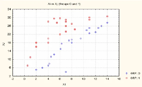
. Figure 1 illustrates a typical situation where this phenomenon occurs.
Fig 1 - Illustration of data conditions unfavorable for forward stepwise selection methods (two-group DA)
It may be noticed that in this case the contribution of Xi and Xj to group separation, is mostly
due to their different within-groups and across-groups correlation patterns, i.e., the fact thatµ −1i µ2i and µ −1j µ2j have opposite signs, although within-groups Xi and Xj are
positively correlated. Data conditions where these patterns differ are particularly unfavor-able for forward stepwise procedures. However, backward stepwise procedures are not so strongly affected by this problem, because these procedures typically start the analysis by a model that includes all candidate variables. In the example described above, from any model including both Xi and Xj, the decrease in group separation due to the removal of one of these
variables would be correctly assessed, and Xi or Xj would not be “good candidates” to leave
the model.
There is however, another problem with stepwise procedures that may affect the performance of procedures based either on forward or backward strategies. This problem concerns the choice of the dimension of the subset(s) to be used in the final analysis. When the contribu-tions to group separation are about evenly distributed among all variables, then any stepwise procedure, may fail to recognize when to stop (since all single variable increments or reductions in group separation will be similar) and suggest variable subsets that are either very small or very large.
It should be remarked that although through the discussion presented above, multivariate normality and equality of variance-covariances were assumed, the fundamental arguments presented should remain valid (although in some different form) in more general problems. In particular, differences in the within-groups and between-groups structure of variable dependence create serious problems for forward stepwise procedures, and individually small contributions to group differences by a large number of variables create difficulties for any stepwise (forward or backward) selection strategy.
VARIABLE SCREENING IN K-GROUP DISCRIMINANT ANALYSIS
Let’s now turn our attention to variable screening for DA problems with more than two groups. In this case there is no single index of group separation with general applicability. Among the several indices proposed for descriptive purposes, one the most widely used is η2
, which may be defined as one minus the proportion of the sample generalized variance(1) that can not be explained by the group differences. Let k denote the number of groups, ng the
number of observations in group g, N =
∑
the total number of observations,= k g g n 1 g x and x the
group g, and overall sample centroids, and W = (N-k)S, B = ( )( )'
1 x x x xg− g−
∑
= k g g n , T = W+Bthe within-groups, between-groups and total SSCP matrices of deviations from xg (W) and x (B and T). Then, η2 = 1 - |W| / |T| = 1 - Λ, where Λ is the well known Wilk’s statistic,
concerning the null hypothesis of equal group means. McCabe (1975) has adapted Furnival algorithm to the comparison of variable subsets in DA, according to η2 (2)
. For that purpose the basic algorithm needs to be applied simultaneously to matrices W and T. After each symmetric sweep, the value of can be computed based on the updated determinants
and . As η ηS a 2 | W | S a |T |Sa 2
never increases with the removal of variables, the more efficient “leaps and bounds” approach of Furnival and Wilson can also be employed. Computer experiments show that replacing Furnival algorithm by Furnival and Wilson’s can lead to impressive reductions in computational effort.
Another common index of group separation is the index W proposed by Rao (1952, pp 257),
W = ng g k (Xg X) 'S (X X 1 g − − =
∑
1 )− , which is an weighted sum of sample Mahalanobis distances between each group centroid and the overall centroid across all groups. The adaptation of Furnival and Wilson algorithm to subset comparisons based on this index offers no difficulties. We notice that W always increases with the addition of new variables and may be expressed as a sum of k quadratic forms Q(g)(.) based on the vectors vS(g) =
1 Xg− X
and common symmetric matrix M = S, satisfying conditions (A) and (B). In this case, the
k quadratic forms can be evaluated simultaneously if the usual MV(.) matrices are augmented
with one raw and column for each (3)
S S1 1
vS(g)
a .
Geisser (1977) and McCulloch (1986) studied the problem of measuring group separation, when the original data is projected into a space of dimension q (q ≤ r = min(p,k-1)). These authors proposed a class of separatory measures consisting on all increasing functions of the
q first eigenvalues of (Γ-∑)) ∑-1 (Γ being the total variance-covariance of X). Replacing Γ
and ∑ by their sample estimates these measures lead to indices of separation based on the first q eigenvalues of BW-1,
λ1, λ2, ..., λq. It can be shown that η2 and W are two particular cases of such indices, as η2
=1 - 1 1 1 + =
∏
λ j i r , W = (N-k) λi, and η i r =∑
1 2, W are indices that consider all possible dimensions
of group separation. When all important group differences can be described by the first q linear discriminant functions, indices of group separation in the space generated by these functions, can be defined using versions of the usual indices, that ignore the last r - q
eigenvalues of BW-1. Alternatively, when it is particularly important to ensure that all dimensions of group-separation are correctly represented, a reasonable comparison criterion is λq, an index of the separation associated with the least dimension with importance.
Unfortunately, Furnival algorithm can not be easily adapted to the repeated evaluation of λi
(i=1,2,...,q). However, if r ≤ 3 (typically problems with four or less groups) there is a way of computing the eigenvalues λi, from determinants and quadratic forms satisfying conditions
(A)- (B), and all indices based on Geisser and McCulloch measures can be used as criteria in efficient all-subsets comparison procedures. Considering known relations between DA and Canonical Correlation Analysis (CCA), the λi can be presented as particular functions of
canonical correlations. The adaptation of Furnival and Furnival and Wilson algorithms to the evaluation of λi, will be discussed latter, under the more general context of subset
compari-sons in CCA.
For DA problems involving more than two groups there is no simple relation between descriptive measures of group separation and estimates of prediction power. Schervish (1981) has proposed parametric estimators of hit rates, valid for the general k-group DA problem as long as the traditional assumptions hold. However, the computation of the resulting estimates requires the evaluation of k-1 dimensional integrals and Schervish estimators are not commonly used in practice. The estimation of prediction power in a k-group setting (k > 2) is usually based on non-parametric estimators that use some combina-tion of “counting” and cross-validacombina-tion strategies. As the computacombina-tional burden required by both parametric and non-parametric estimators of hit rates is important, often it is not feasible to make all-subsets comparisons based on direct measures of prediction ability. Thus, in order to avoid the dangers of stepwise procedures one possibility is to use some index of group separation as a proxy for prediction ability. However, global indices of separation like η2
or W are usually strongly influenced by the groups that are further apart, while prediction ability is mostly dependent on the separation between the groups that are closer together (McLachlan 1992, pp 93). An index that does not suffer from this problem is the smallest sample Mahalanobis distance between all pairs of groups. This index is used as a comparison criterion by one of the stepwise selection routines of SPSS. Furnival and Wilson algorithm can be easily adapted for subsets comparisons based on this criterion, by defining as S and creating different vectors, one for each pair of differences in sample group centroids.
MS S1 1
C2k vS1
The characterization of the problems of stepwise procedures, presented previously in the context of two-group DA, generalizes naturally to k-group problems. In particular, the discussion presented applies directly to any measure based on Mahalanobis distances, like the population analogue of W or the distance between the two closest groups. If group separa-tion is understood as a funcsepara-tion of unexplained variance, measured by a populasepara-tion analogue of η2
, then some insight can be gained from following argument. Suppose that Xk is added
to an analysis based on a subset Sa. Then the population counterpart of 1- η2 is multiplied by
a factor c (8) which is simply the ratio between the within-groups and total conditional variances of Xk (given Sa). c = k S S S S k kk k S S S S k kk a a a a a a a a , 1 , , 1 , Γ Γ Γ Γ Σ Σ Σ Σ − − − − (8)
One of the principal problems of forward stepwise selection methods, is the fact that they ignore the correlations between variables currently out of the analysis. The consequences of this problem are bound to be more serious when these correlations have different impacts in the total and within-groups conditional variances. The occurrence of such different impacts is usually a consequence of differences in the within-groups and across-groups correlation structures. Finally, the problems of stepwise methods in finding an appropriate subset dimension, affect two-group and k-group DA problems in the same manner.
VARIABLE SCREENING IN MANOVA AND MANCOVA Consider the general MANOVA (9) and MANCOVA (10) models:
Y = X Π + U (9)
Y = X Π + Z Ψ + U (10)
where Y is a (n*p) matrix of responses, X is a (n*q) design matrix, Z is a (n*t) matrix of covariates, U is a (n*p) matrix of error terms and Π, Ψ are (q*p) and (t*p) matrices of unknown parameters. In this section, the problem of comparing the subsets, Sa, of Y
according to their contribution to an “effect” characterized by the violation of a linear hypothesis H0: A Π = 0, will be discussed.
General linear hypothesis A Π C = 0, with C different of the (p*p) identity (I) will not be considered because of the following two reasons: (i) Usually, it only makes sense to select variable subsets concerning hypothesis that do not involve linear combinations of parameters associated with different variables. When such hypothesis are present (for instance, in the MANOVA approach to the analysis of repeated measurements) often all the response variables have substantive importance and none should be removed. (ii) Even when it makes sense to select subsets of Y concerning an hypothesis A Π C = 0 (C ≠ I) , usually it is not possible to find an appropriate criterion based on a matrix, M, satisfying condition (A) . The usual test statistics concerning the hypothesis H0 include Wilk’s lambda
(Λ = |E| / |T|), Bartlett-Pillai trace (U = tr H T-1
) and Hotelling-Lawley trace (V =
tr H E-1), where H, E and T = H + E are Hypothesis, Error and Total SSCP matrices (see e.g., Seber 1984, Ch. 9) concerning H0. For the purpose of subset comparisons it is
conven-ient to measure the extent of H0 violations by an appropriate index of the magnitude of the
associated effect. Several such indices may be defined, often as a function of the rank of the matrix H (r), and the value of some test statistic. For instance, three usual indices of effect magnitude are τ2 = 1 - Λ1/r, ξ2
= U/r and ς2
= V / (V+r).
It may be noticed that Descriptive DA can be presented within this framework. For instance, the problems covered in the previous sections are related to a MANOVA model (9) where the design matrix X implies a one-way layout. In that case the hypothesis H0 concerns the
equality of group means and the associated effect may be described as “group separation”. The corresponding SSCP matrices are respectively
E = W and H = B and the rank of H equals the minimum between the number of responses and number of groups minus one (r = min(p,k-1)). However, the discussion to be presented in this section is more general, because on the one hand it allows for the presence of
covari-ates, and on the other hand it admits subset comparisons according to their contribution to other effects, like specific contrasts or factor interactions in a multi-way layout.
Furnival and Wilson algorithm can be adapted to subset comparisons based on any criterion that can be expressed as a function of the value of the statistics, Λ, U or V. First, notice that for an hypothesis A Π = 0, all three matrices H, E and T satisfy condition (A). Furthermore, when a variable Yk is removed from a subset Sb, the value of Λ always increases and the
values of U and V always decrease. Subset comparisons based on Λ (or more appropriately on τ2
) follow from a direct application of McCabe (1975) strategy to the matrices E and T, replacing Furnival algorithm by Furnival and Wilson’s. To show that this algorithm can also be applied to subset comparisons based on criteria derived from U or V, it suffices to show that these statistics can be expressed as sums of quadratic forms Q(i)(.). Let be the spectral decomposition of H. Then, U can be expressed alternatively as U =
θi i r h hi i' =
∑
1 tr H T-1 = tr i = i r θ h hi i' T = −∑
⎛ ⎝ ⎜ ⎞⎠⎟ ⎡ ⎣ ⎢ ⎤ ⎦ ⎥ 1 1(
θ) (
θ i i r i hi T h 1 i ' − =∑
1)
where θi is the i-th eigenvalue
of H and hi the corresponding normalized eigenvector. Thus, the adaptation of Furnival and
Wilson algorithm simply requires an evaluation of the sums based on the matrix = T, and vectors = Q i r (i) (.) =
∑
1 MS S1 1 vS (i)1 θi hi,. Using a similar argument, subset comparisons based
on criteria derived from V = tr H E-1 can be easily made if and are defined as E and MS S 1 1 vS (i) 1 θi hi.
Stepwise selection methods in MANOVA and MANCOVA are usually based on Roy’s additional information criterion, (11), (Rao 1973) which measures the contribution of Y
a
S k|
Λ
k to the effect under study, when the influence of the variables included in Sa is factored
out. k , S 1 S S S k, kk k , S 1 S S S k, kk a a a a a a a a T T T T E E E E − − − − = Λ a S k . (11)
The denominator of (11) is proportional to the sample conditional variance of Yk, and the
numerator can be interpreted as the portion of Yk ‘s sample conditional inertia that is not
related to the effect. Considering the population equivalents to E and T, it can be argued that forward stepwise methods are more prune to miss good subsets when there are important differences between the correlation structures related and unrelated to the effect under study. On the other hand, both forward and backward stepwise procedures may have problems identifying appropriate subset dimensions, particularly when the effect contributions are about evenly distributed by a large number of different variables.
VARIABLE SCREENING IN CANONICAL CORRELATION ANALYSIS
Canonical Correlation Analysis (CCA) is traditionally described as a technique to study the relations between two sets of variables. This view of CCA has interest in applications where two different concepts are measured by several variables, for example, a medical researcher
$
ρ
studying the relation between sets of variables describing eating habits and heart conditions or a financial analyst trying to relate ratios of capital structure to measures of profitability. However, the role of CCA in multivariate statistics is not restricted to its use as a multivariate technique on its own. The theory of CCA is particularly important because it provides a unifying framework for several multivariate methodologies. If effect, Discriminant Analysis, Multivariate Regression Analysis, MANOVA and MANCOVA can all be presented as particular cases of CCA.
In the first part of this section, variable screening will be discussed within the context of CCA as a technique on its own. In the second part, the relations between CCA and other methodologies will be explored, showing how the results presented in the first part relate to and sometimes extend, the methods of variable screening discussed in the previous sections. Let X = {X1,X2,...,Xq} and Y= {Y1,Y2,...,Yp} be two sets of variables and denote the
dimension of the smaller set by r = min(q, p). Suppose that one of these sets, say X, is fixed and it is desired to compare the subsets, Sa, of the other set, Y, according to some measure of
association between Sa and X. Several measures of multivariate association have been
proposed in the literature. Cramer and Nicewander (1979) argue that good measures of association should be invariant to linear transformations, and symmetric, i.e., should not be affected by a reversal in the roles played by the X and Y sets. These authors discuss seven alternative measures with those properties, all of which are functions of sample squared canonical correlations (ρ$i2 ) between X and Y.
The measures considered by Cramer and Nicewander are the following: $ ρ1 2 , γ$1 2 , ; 1 = =
∏
i i r $ ( $ ) γ2 ρ 2 1 1 1 = − − =∏
i i r $ ( $ ) γ ρ 3 2 1 1 1 1 = − − =∑
r i i r ; ; ; $ $ / γ 4 ρ 2 1 1 =⎡ ⎣ ⎢ ⎤ ⎦ ⎥ =∏
i i r r $ ( $ ) / γ5 ρ2 1 1 1 1 = −⎡ − ⎣ ⎢ ⎤ ⎦ ⎥ =∏
i i r r $ $ γ ρ 6 2 1 =∑
i= i r rFor the purpose of subset comparisons these measures result in five alternative criteria asγ$1 , $
γ4 and γ$2 , γ$5 are monotically related (γ$4 =$ ; ). / γ11 r $ ( $ ) / γ5 γ2 1 1 1 = − − r
The first squared canonical correlation, , measures the linear association between the maximally correlated linear combinations of X and Y. Therefore, is an appropriate measure of multivariate association, when it reasonable to assume that each set of variables can be summarized along one single dimension. All the other measures consider the r possible dimensions along which X and Y may be associated. The measure
$ ρ12 $ ρ12 $ γ1 was initially
proposed (in slightly different contexts) by Hotelling (1936) and Cramer (1974). Its use can be justified by the following argument. Suppose that the values of the r variables belonging to the smaller set, are predicted by linear regressions on the variables belonging to the larger set. Then, it can be shown that the ratio between the generalized variances of the predicted and observed values equals γ$1 . In that sense, γ$1 can be interpreted as a multivariate generalization of the coefficient of determination, R2. The use of γ$4 is justified by noting that while a (univariate) variance can be described in terms of a vector’s squared-length, a generalized variance has an equivalent interpretation in terms of the squared-volume of a parallelotope (Anderson 1958). Thus, replacing γ$1 by γ$4 is equivalent to replacing the ratio
between two squared-volumes by the ratio between the side squared-lengths of the hyper-cubes with the same volume as the original parallelotopes (Cramer and Nicewander 1979, pp 49). The measureγ$2 was proposed by Hotelling (1936) and Rozebom (1965), and can be justified along similar lines to γ$1 . In effect, γ$2 is also a natural generalization of R2 for the regressions of the variables in the smaller set on the variables of the larger set. It may be shown that in this case,γ$2 equals one minus the ratio between the generalized variances of the residuals and the observed values. However, γ$2 is not equal toγ$1 because in multivari-ate regression the generalized variances of the residuals and predicted values do not add up to the generalized variance of the observed values. The use of γ$5 instead of γ$2 follows from the same argument that justifies replacing γ$1 by γ$4 . The measure γˆ3 was proposed independently by Coxhead (1974) and Shaffer and Gillo (1974). Assuming the same set of linear regressions as previously, it can be shown that the ratio between the sums of the predicted and observed squared-distances (according to a Mahalanobis metric) between all pairs of observations, equals γˆ3 . The measure γˆ6 is the average of the squared canonical correlations and is the measure preferred by Crammer and Nicewander because, among other reasons, of its simplicity. Additional desirable properties of γ$6 are discussed in Crammer and Nicewander (1979) article.
In order to adapt Furnival and Wilson algorithm to subset comparisons based on the measures described above, we first note that none of these measures can increase when variables are removed. Furthermore, it can be shown that if the Y variables are regressed on the X variables, then ρ$i2 equals the i-th principal eigenvalue of 1
YY Y Y S
S ˆ ˆ − where SYY$ $ and SYY are the sample variance-covariance matrices of the predicted and observed Y values (conversely, when the X’s are regressed on the Y’s, equals the i-th eigenvalue of ). There-fore, noting that the i-th eigenvalues of
$ ρi2 1 XX X X S S − ˆ ˆ 1 YY S See − and 1 YY Y Y S
S ˆˆ − (where See denotes the
variance-covariance matrix of the residuals for the regressions of Y on X) add up to one, $
γ2 may be expressed asγ$2 = 1 - |See| / |Syy|. Thus, efficient subset comparisons based on
$
γ2 (or γ$5 ) only require applying McCabe strategy simultaneously to the matrices See and
Syy. Comparisons based on γ$3 , follow from γ$3 = tr ( 1
Y Y See
S ˆˆ − ) / tr ( 1 YYSee S − ) = tr( 1) / [r + tr ( ) ]. Using the spectral decomposition of , tr(
Y Y See S ˆ ˆ − 1 Y Y See S ˆˆ − SYˆYˆ 1 Y Y See S ˆ ˆ − ) can be expressed as a sum of r quadratic forms v ' MS(i) S S1 vS(i), where equals S
1 1 1
−
1 MS S1 1 ee and
is an eigenvector of S . Then, the adaptation of Furnival and Wilson algorithm is straightforward. Efficient subset comparisons based on
vS(i)
1 YY$ $
$
γ6 can also be made without any major difficulty. Noting that γ$6 = tr ( 1
YY Y Y S
S ˆˆ − ) / r, and using the spectral decomposition of , can also be expressed as a sum of quadratic forms, Q
SYY$ $ rγˆ6 (i)(.), and the usual procedure
follows.
Efficient subset comparisons based on γ$1 (γ$4 ) or are not as straightforward, as those based on the other measures. If p = min(p,q) = r, i.e., if the number of variables under comparison (Y) does not exceed the dimension of the fixed set (X), then
$
ρ12
$
γ1 = | SYY$ $ | / |SYY| and subset comparisons based on γ$1 (orγ$4 ) can be made by a simple adaptation of McCabe (1975) algorithm. However, in most applications p is larger than q, which implies that |SYY$ $|
= 0, and γ$1 can not be easily expressed as a ratio of determinants. As far as we can tell, there is no general way of adapting Furnival and Furnival and Wilson algorithms to subset comparisons based on γ$1 ,γ$4 or . However, in some special cases it is possible to take advantage of known relations between traces and determinants, in order to compute all (or some) canonical correlations for the subsets under comparison. For instance, if r ≤ 3 the known relations Λ = = |S $ ρ12 − =
∏
(1 $ )2 1 ρi i r ee| / |Syy|, U = ρ$i = tr( ), V = 2 i r =∑
1 1 YY Y Y S S ˆˆ −(
)
∑
= ρ − ρ r i 2 i 2 i (1 ) 1 ˆˆ = tr( ), (where Λ, U and V denote the values of Wilk’s, Bartlett-Pillai and Hotelling-Lawley statistics concerning the null hypothesis of no association between the X and Y sets), can be used to compute all . After some tedious algebra it follows that for r = 2, the values of and are given by equation (12) and for r = 3,
, and are the three solutions of equation (13). 1 Y Y See S ˆ ˆ − $ ρi 2 $ ρ1 2 ρ$ 2 2 $ ρ1 2 ρ$ 2 2 ρ$ 3 2 r = 2 ⇒ ρ$i2 1
(
U U2 (U ))
2 4 1 = ± − + −Λ (12) r = 3 ⇒ (ρ$1) 2 3 - U (ρ$1) 2 2 + [2U-3 + Λ(V+3)] ( ) + 2-U-Λ(V+2) = 0 (13) $ ρ1 2The results presented above, have important implications in other multivariate techniques rather than CCA on its own. For instance, it is well known that k-group descriptive DA can be presented has the CCA between p variables describing entity attributes, and k-1 indicator variables describing group membership (McLachlan 1992, pp 185-187). In that case,
and BW 1
Y Y See
S ˆˆ − -1 have the same positive eigenvalues (λi) and the measure γ$2 is the usual
η2
index. Furthermore the squared canonical correlations are related to the eigenvalues of BW-1 by the equation λi = ρ$i
(
ρ$i)
2 2
1− .
Consider now the MANOVA (9) and MANCOVA (10) models. Denote the space spanned by the columns of X (MANOVA) or X and Z (MANCOVA) by Ω, the subspace of Ω defined by the hypothesis H0:A Π = 0 by ω, the orthogonal complement of ω by ω⊥ and the space
spanned by the projection of Y on ω⊥ by γ. Then, the analysis of H
0 can be presented in
terms of a CCA between two sets of vectors spanning γ and Ω (Masson 1990). In this case, and HE
1 Y Y See
S ˆˆ − -1 have the same positive eigenvalues, the γ$3 ,γ$5 , γ$6 measures are the usual ς2, τ2 and ξ2 indices, and the rank of H, r, equals the minimum between p and the dimension of
ωp = ω⊥ ∩ Ω. When r ≤ 3, Furnival algorithm can be adapted for subset comparisons based
on any function of the r non-zero eigenvalues of HE-1 (λi), or HT-1 ( ), since if r=1, =
U = tr HT $ ρi2 $ ρ12 -1
, λ1 = V = tr HE-1, and if 1 < r ≤ 3 equations (12) or (13) hold.
COMPUTATIONAL EFFORT
The evaluation of the computational effort required by all-subsets comparison algorithms is usually based on the number floating point operations performed. In the case of the algo-rithms discussed in this article the following three questions are particularly relevant: (i) What is the effort required by algorithms based on Furnival’s (or McCabe’s) exhaustive evaluation of all quadratic forms Q(.) and/or determinants D(.) ? (ii) What are the
computa-tional savings when an exhaustive search is replaced by Furnival and Wilson implicit enumeration algorithm ? (iii) What is the effort required to convert quadratic forms and determinants to appropriate comparison criteria ?
For question (i) exact answers can be found. In effect, as discussed in section 2, Furnival algorithm consists essentially on a succession of symmetric sweeps on portions of
(p+1)*(p+1) matrices, MV(.), or p*p matrices MD(.) with 2p-t-1 different sweeps involving t additional variables (t = 0,...,p-1). As the number of floating point operations required by each sweep is a quadratic function on t, the evaluation of the computational effort for the different versions of Furnivals’s algorithm can be made with the help of the known results on the summations 2 , , presented in equations (14)-(16).
0 1 − = −
∑
t t p t t t p 2 0 1 − = −∑
t t t p 2 0 1 2− = −∑
( )
2 2 1 2 1 0 1 − − = − = −∑
t p t p (14)( )
t t p t p 2 2 1 2 1 0 1 − − = − = − +∑
( p 1) (15)( )
( )
( )
t t p p p p t p 2 1 2 2 0 1 2− 6 1 2 − 1 2 − 3 1 2 = − = − − −∑
p−1 (16)In particular, for the evaluation of quadratic forms, each sweep requires (t+1)(t+4)/2 = 1/2 (t2
+ 5t + 4) operations, and after some trivial computations, it follows that the total number of
floating point operations required is of the order 6(2p). This result is relevant for subset comparisons in linear regression, and two-group DA comparisons based on D2 or on parametric hit rate estimates. Subset comparisons in k-group DA, MANOVA, MANCOVA or CCA based on any function of Bartlett-Pillai U or Hotelling-Lawley V require the evaluation of r quadratic forms with the same symmetric matrix. In that case each sweep requires t (t+3)/2+ (t+2) r = 1/2 [t2 + (3 + 2r) t + 4r] operations, and the total number of
operations is of the order (3+3r)(2p). Subset comparisons based on the smallest Mahalanobis distance in k-group DA, require the evaluation of C quadratic forms. In this case each sweep requires t(t+3)/2 + (t+2) = k 2 Ck 2 1 2
[
(
3 2)
4]
2 2 / t + + Ck t+ 2 Ckoperations, and the total number of operations is of the order
(
3 3+ C2)( )
k
2p . Subset comparisons based on functions of Wilk’s Λ (like the η2
, τ2 indices in k-group DA, MANOVA or MANCOVA, or equivalently the $
γ2 or γ$5 measures in CCA) require the evaluation of all determinants D(.), for two different sets of matrices MD(.). Each sweep in MacCabe’s adaptation of Furnival’s algorithm requires t(t+3)/2 + 1 = 1/2 (t2+3t+2) operations, and the total number of operations for each
set of matrices is of the order 4(2p). Thus, the effort required for the evaluation of Λ for all variable subsets is of the order 8(2p). In three-group DA, MANOVA, MANCOVA or CCA with r=2, subset comparisons based on ρ$12 or ρ$ (λ
2 2
1 or λ2), can be made using equation (12),
which requires finding the values of Λ and U. Noticing that the repeated evaluation of these two statistics require sweeps on the same matrix (T or SYY) some computation savings can be
achieved. In effect, after sweeping the MD(.) matrices used in the evaluation of , only the
r last rows of the MV(.) matrix associated with U need to be updated. Therefore, each
sweep in the simultaneous evaluation of Λ and U requires t (t+3+r) + 2 (1 + r) = t ΛSa Sa
2
+ 5 t + 6 operations and the total number of operations is of the order 14(2p). Finally, subset
compari-sons based on any function of ρ$12 , ρ$22 , ρ$32 (λ1, λ2 , λ3) in four-group DA, MANOVA,
MANCOVA or CCA with r = 3, can be made after solving equation (13), which requires the simultaneous evaluation of Λ, U and V. Noting that the two matrices required for computing all , are exactly the same matrices used in the evaluation of U and V , it follows that in this case each sweep requires t (t+3+2r) + 2(1+2r) = t
ΛSa Sa Sa
2
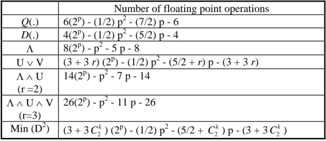
+ 9 t + 14 operations and the total number of operations is of the order 26(2p). Table 1 presents the exact number of floating operations required by all the versions of Furnival algorithm discussed in this article.
TABLE 1: Computational effort required by exhaustive comparison procedures based on Furnival algorithm
Number of floating point operations
Q(.) 6(2p) - (1/2) p2 - (7/2) p - 6 D(.) 4(2p) - (1/2) p2 - (5/2) p - 4 Λ 8(2p) - p2 - 5 p - 8 U ∨ V (3 + 3 r) (2p) - (1/2) p2 - (5/2 + r) p - (3 + 3 r) Λ ∧ U (r =2) 14(2p) - p2 - 7 p - 14 Λ ∧ U ∧ V (r=3) 26(2p) - p2 - 11 p - 26 Min (D2) (3 + 3Ck) (2 2 p ) - (1/2) p2 - (5/2 + C2k) p - (3 + 3C ) k 2
Question (ii) can not be answered exactly because the portion of Furnival and Wilson’s search tree that can be pruned is dependent on the configuration of the sample data. In particular, when different sets of variables have highly different impacts over the comparison criterion, C(.), it is relatively easy to identify “the best” subsets early on, and large parcels of the search tree can be pruned. On the other hand, when all the variables have similar contributions to C(.), it is more difficult to eliminate subsets and the computational savings tend to be smaller. In spite of this difficulty, a rough idea of the computational burden for some typical and worst case scenarios can be given based on simulation experiments. For instance, Furnival and Wilson (1974) report that in a series of trials to find the 10 best subsets of each dimension, in regression models, the number of operations performed was equal to 3,764 (p=10), 123,412 (p=20), 3,934,714 (p=30) and 11,614,024 (p=35). These figures correspond to 62.18%, 1.19%, 0.06% and 0.005% of the number of operations that would be required to compare all subsets using Furnival algorithm. Duarte Silva (forthcoming) in a series of trials to identify the 20 best subsets according to McLachlan (1974) hit rate estimate in two-group DA, reports a number of operations in the range 3,619 - 4,494 (p=10), 117,143 - 557,660 (p=20) and 7,462,258 - 57,380,009 (p=30) which correspond respectively to 61% - 74% (p=10), 1.86% - 8.86% (p=20), and 0.15% - 0.89% (p=30) of the effort that would be required by Furnival algorithm. Duarte Silva experiments refer to worst case scenarios where all variables were generated from populations where these variables had equal discriminatory power. A few trials with other procedures revealed efforts of similar orders of magnitude. In particular, for p ≥ 30, comparison procedures based on Furnival and Wilson algorithm are
typically faster than procedures based on Furnival algorithm, at least by a factor of 100, and as p grows this factor quickly becomes larger than 1000.
All the analysis presented in the previous paragraphs considered the number of operations involved in the computation of quadratic forms, Q(.), and/or determinants, D(.), and ignored the effort required to convert Q(.) and D(.) into appropriate comparison criteria, C(.). However, using efficient implementations, it is usually possible to minimize the number of conversions, ensuring that they require a small fraction of the total computational effort. For instance, when C(.) is equal to Q(.) (like the squared Mahalanobis distance in two-group DA, or the smallest squared Mahalanobis distance in k-group DA) or is a monotic function of
Q(.) summations (like Roy’s W index in k-group DA, the ξ2 , ς2 indices in
MANOVA/MANCOVA or theγ$3 ,γ$6 measures in CCA), subset comparisons can be made directly on Q(.), and no conversion is required for that purpose. Even if the final results are presented in terms of C(.), conversions are required only for the pool of subsets selected for further analysis, which for pratical reasons should never include more than a few hundred subsets.
In two-group DA problems, for subsets of equal dimensions, comparisons based on paramet-ric estimates of the hit rate are equivalent to comparisons based on the sample Mahalanobis distance and do not require any conversion from Q(.) to C(.). However, that is no longer the case for comparisons across subsets of different dimensions. In that case, the number of conversions can be minimized if for each subset, Sa, Q(Sa) = is compared against the
largest squared Mahalanobis distance for the subsets of the same dimension, already excluded from the list of candidates for further analysis. Only when Q(S
DS
a
2
a) exceeds this value, a
conversion from Q(Sa) to C(Sa) is required. Some computational experiments show that for
values of p around 30, while the evaluation of the Q(.) typically require a few million operations, the number of conversions usually does not exceed a few hundred. Thus, even when relatively expensive estimates are chosen for C(.), these conversions still remain a small fraction of the total effort.
Subset comparisons based on monotic functions of Wilk’s Λ statistic can be made using the same the number of operations as those required to compute the determinants and | |. In effect, if MD
|ES |
a TSa
(1)
(.) and MD(2)(.) are the matrices derived respectively from E and T, in McCabe’s adaptation of Furnival’s algorithm, at each sweep the value of Λ can be updated directly using the relation = * (MD
b
S
Λ ΛSa
(1)
(Sa)kk / MD(2)/ (Sa)kk) which only requires two
operations.
In DA, MANOVA/MANCOVA and CCA problems with r = 2, subset comparisons based on a arbitrary function of and require solving equation (12) which involves three operations and the extraction of a square root. However, for many special cases this effort can be reduced. For instance, if C(.) is a monotic function of , then the computation of
can be skipped which saves one floating point operation. Furthermore, the relation $ ρ12 $ ρ22 $ ρ12 $ ρ22
(
USi>USj) (
∧
Λ <Si ΛSj)
⇒ρ$1 >ρ$ 2 1 2Si Sj can be used in order to minimize the number of conver-sions. Conversely, if C(.) is a monotic function of , the number of conversions can be reduced noting that
$ ρ2 2
(
USi>USj) (
∧
1/4(USi −USj)+( Sj− Si)<USi−USj)
2 2 Λ Λ ⇒ . $ $ ρ2 ρ 2 2 2 Si > SjThe evaluation of , and in DA, MANOVA/MANCOVA and CCA problems with r = 3, involves solving the third-degree equation (13). In our current implementation, equation (13) is solved by the Newton-Raphson method. However, for common C(.), based on the
$ ρ12 $ ρ22 $ρ3 2
behavior of the function defined by the left hand side of (13), and noting that 0 ≤ ≤ ≤ ≤ 1, it is often possible to avoid unnecessary conversions.
$ρ3 2 $ ρ2 2 $ ρ1 2
The principal justification for the analysis of computational effort presented in this section, is to have an idea the number of candidate variables, p for which the procedures presented in this article, are feasible within a “reasonable” time. Two different views of “reasonable” will be adopted. In the first view, directed to on-line analysis, the computational time will be considered as “reasonable” if it does not exceed three minutes. In the second view, directed to batch analysis, the computational time will be considered as “reasonable” if it does not exceed 48 hours (what might be called a “week-end analysis”). In modern personal com-puters, the number of floating point operation performed per second typically varies between one hundred thousand and one million. Thus, the limit on the number of operations for on-line all subset comparisons should lie somewhere in the range 18 - 180 millions. Assuming that for the largest on-line analysis, Furnival and Wilson algorithm is about 1000 times faster than Furnival’s, and ignoring the overhead and conversion effort (which for problems of this size is reasonable), the maximum number of candidate variables that can be analyzed on-line, should be in the range 30-35. “Week-end” batch analysis can be performed as long as the number of operations required is not above 17-170 billions. Assuming that for the largest problems, Furnival and Wilson algorithm is about 100,000 times faster than Furnival’s, the maximum allowable value for p should be around 45-50. Obviously, these figures should be interpreted only as rough estimates, since the true limit on p depends on many factors, such as the type of computer used, analysis performed, criteria chosen and data configuration. When this limit is exceeded, a viable alternative, is to use either judgment, substantive knowledge, or stepwise selection methods (if the data conditions are not particularly unfavorable) in order to reduce the number of candidate variables to a manageable size, and then employ an all-subsets comparison procedure.