Equity valuation of Hugo Boss AG

(1)

Equity Valuation of Hugo

Boss AG

Denis Zimmerer

Dissertation written under the supervision of José Carlos Tudela

Martins

Dissertation submitted in partial fulfilment of requirements for the MSc in

Finance, at the Universidade Católica Portuguesa, 07 June 2019.

(2)

i

HUGO BOSS AG Recommendation Buy

Deutsche Börse AG Current Share Price € 62.50 (07.03.2019)

Premium Apparel Target Share Price € 87.86 (31.12.2018)

Valuation Metrics INVESTMENT SUMMARY

2019E EV/EBITDA 82.96 WACC 6.09% Cost of Equity 6.34% Cost of Debt 0.62% Tax Rate 29.55%

Perpetuity Growth Rate 2.16% 5-Year EBIT Margin (avg.) 12.66%

Capital Market Data

as of 07/03/2019

Share Price (€) 62.5

52 Weeks High (€) 81.4 52 Weeks Low (€) 52.54 Annualized Volatility 27.44% Shares Issued (mil.) 69.02 Free Float (mil.) 61.89 Market Cap (€, bil.) 3.66

Indexed Weekly Performance

-5Y Stock Performance

Close Pr. BOSSn.DE MDAX 1 Week -7.50% -1.52% 1 Months -16.18% -4.87% 1 Year -32.23% -5.89% 5 Years -34.71% 46.16%

Key Financials

€, million 2016 2017 2018 2019E 2020E 2021E 2022E 2023E

Revenue 2,693 2,733 2,796 2,872 2,960 3,058 3,166 3,278 EBIT 263 341 347 364 375 387 401 415 as % of sales 9.77% 12.48% 12.41% 12.66% 12.66% 12.66% 12.66% 12.66% EBITDA 402 474 470 504 519 535 553 571 FCFF 120 325 160 184 210 207 212 247 EPS (€) 2.80 3.35 3.42 3.57 3.69 3.81 3.94 4.07 ROA 17.63% 13.40% 12.61% 12.55% 12.52% 12.46% 12.37% 12.31% ROE 35.74% 25.18% 23.90% 23.93% 23.54% 23.21% 22.87% 22.58% 0,30 0,80 1,30 20 14 20 15 20 16 20 17 20 18 BOSS MDAX Buy

A buy recommendation is issued to Hugo Boss AG due to a target price between €81.15/share to €87.86/share which reflects an upside of 29.84% to 40.57% to the current market price of €62.50/share.

Market

The luxury and premium apparel market is expected to grow especially due to higher demand in Asia. Hugo Boss benefits from this particular development and a 5year CAGR of 2.82% is expected. This development is underpinned by Hugo Boss achievment of reaching its targets in 2018 besides the difficult market situation for european retailers.

Distribution_Channel

Hugo Boss will keep on improving their own retail sales by opening new retail stores and restructuring old ones. Furthermore, they will keep on investing into their online-channel, which should be rewarded with higher sales. However, decreasing wholesales are likely to offset the positive effects of its new ditribution strategy. Therefore, the managements forecast of a 15% EBIT-margin until 2022 seems too ambitious.

(3)

ii

Abstract

The purpose of this dissertation is to evaluate the fair price per share of the German premium apparel manufacturer Hugo Boss AG and issue a buy, hold or sell recommendation. The valuation will take into account the current macroeconomic environment, several industry outlooks and trends, the company’s historical financial performance and its future strategy. Hugo Boss is evaluated by the intrinsic Discounted Cash Flow method, and complemented by the relative method of Multiples. Thus, a fair value between €81.15/share to €87.86/share is issued. This reflects an upside of 29.84% to 40.57% compared to the traded price of €62.50/share and concludes a buy recommendation.

Title: Equity Valuation of Hugo Boss AG

Author: Denis Zimmerer

Keywords: Corporate Finance, Equity Valuation, Hugo Boss, Premium Apparel Industry

Resumo

O objetivo desta dissertação é avaliar o “fair value” por ação do produtor Alemão de roupas premium Hugo Boss AG e emitir uma recomendação para “comprar, manter ou vender”. A avaliação da empresa terá em conta o ambiente macroeconómico atual, várias perspetivas e tendências do setor, o desempenho financeiro histórico da empresa e a sua futura estratégia. Hugo Boss é avaliada pelo método de Fluxo de Caixa Descontado intrínseco e complementado pelo método de Múltiplos relativo. Assim, um justo valor entre €81.15/ação e €87.86/ação é emitido. Isto reflete um aumento de 29.84% para 40.57% em relação ao preço negociado de €62.50/ação e conclui uma recomendação de “compra”.

Título: Equity Valuation of Hugo Boss AG

Autor: Denis Zimmerer

(4)

iii

Acknowledgment

This dissertation marks the final steps in completing my academic education. First and foremost, I would like to thank my family for their unconditional support, love and encouragement, without whom I would not have been able to overcome difficult hurdles. Moreover I would like to say a big “thank you” to my girlfriend Franziska Welp, who always supported me and enlightend the times I had to spend away from home, no matter which distance seperated us.

Furthermore, many thanks to all my dear friends at university, who always offered their help and made this whole experience so enjoyable. Therefore, I would like to especially highlight Martin Kreuzer, Marcin Rękawiczny, Lorenzo Candotto, Felix Cord and Simone Pesce. Last but not least, a great thank you to my supervisor José Carlos Tudela Martins, who always gave me critical feedback, and supported me in writing this thesis.

(5)

iv

Table of Formulas

Formula 1: Net Present Value ... 2

Formula 2: Free Cash Flow to the Firm ... 3

Formula 3: Free Cash Flow to the Equity, starting at FCFF ... 4

Formula 4:Free Cashflow to the Equity, starting with Net Income ... 5

Formula 5: Unlevered Cost of Equity ... 6

Formula 6: Present Value of Interest Tax Sield ... 6

Formula 7: PV Expected Bankruptcy Cost ... 6

Formula 8: Present Value of Terminal Value ... 7

Formula 9: Weighted Average Cost of Capital ... 9

Formula 10: Capital Asset Pricing Model ... 10

Formula 11: Fama French Three Factor Model ... 10

Formula 12: Regression for Beta ... 11

Formula 13: Unlevered Beta ... 11

Formula 14: Blume Beta Adjustment ... 11

Formula 15: Price-Earnings-Ratio ... 13

(9)

viii

Table of Figures

Figure 1: IMF GDP growth rates... 16

Figure 2: Current Yield Curves ... 16

Figure 3: Inflation Rates ... 17

Figure 4: Fashion Industry Sales Growth (McKinsey & BoF, 2018) ... 18

Figure 5: Personal luxury goods industry (Bain & Company, 2019) ... 19

Figure 6: Luxury personal goods segments (Statista 2019) ... 19

Figure 7: Forecasted Growth of HNWI (Statista 2019) ... 21

Figure 8: Forecast tourist arrivals (Statista, 2019) ... 22

Figure 9: Global apparel and footwear sales forecast (McKinsey and BoF 2018) ... 22

Figure 10: Real GDP CAGR forecast (McKinsey and BoF 2019) ... 24

Figure 11: Online sales (Bain & Company 2019) ... 25

Figure 12: Average time to shelf (McKinsey and BoF 2018) ... 27

Figure 13: Share price development Hugo Boss and MDAX (Reuters) ... 29

Figure 14: Comparison Hugo Boss and MDAX ... 30

Figure 15: Sales Distribution Hugo Boss (Hugo Boss, 2019a) ... 31

Figure 16: Operating Results (Hugo Boss, 2019a) ... 34

Figure 17: SWOT Analysis ... 35

Figure 18: Sales Hugo Boss ... 40

Figure 19: Projections of COGS and SGA ... 42

Figure 20: Capex and Depreciation Amortisation ... 44

Figure 21: D&A and PPE plan ... 44

Figure 22: Cost of Equity Inputs ... 47

Figure 23: Inputs Cost of Debt ... 48

Figure 24: Terminal Value Calculation ... 49

Figure 25: Terminal Growth Rate Computation... 49

Figure 26: Long List Peer Companies Selection ... 54

Figure 27: Peer Evaluation ... 55

(10)

ix

Table of Tables

Table 1: Sales by segment and Distribution Channels Hugo Boss ... 32

Table 2: Costs (Hugo Boss 2019a) ... 33

Table 3: DCF Valuation Hugo Boss ... 38

Table 5: Net Working Capital: ... 46

Table 6: WACC Inputs ... 47

Table 7: Equity Value and share price ... 51

Table 8: Sensitivity Analysis ... 52

(11)

x

Table of Abbrevations

APV Adjusted Present Value

CAPM Capital Asset Pricing Model

CAPEX Capital Expenditures

COGS Cost of Goods Sold

CRP Country Risk Premium

D&A Depreciation and Amortisation

DAX30 Deutscher Aktienindex

DCF Discounted Cash Flow

DSO Days Sales Outstanding

DPO Days Payables Outstanding

DPS Dividend per Share

EBIT Earnings Before Interest and Taxes

EBITDA Earnings Before Interest, Taxes, Depreciation and Amortisation

EPS Earnings per Share

ERP Equity Risk Premium

EV Enterprise Value

FCF Free Cash Flow

FCFE Free Cash Flow to the Equity

FCFF Free Cash Flow to the Firm

g Growth Rate

GDP Gross Domestic Product

HNWI High Net Worth Individual

IMF International Monetary Fund

Kd Cost of Debt

Ke Cost of Equity

LTM Last Twelve Month

MDAX Mid-Cap DAX

MRP Market Risk Premium

MVD Market Value of Debt

MVE Market Value of Equity

NOPLAT Net Operating Profit Less Adjusted Taxes

NPV Net Present Value

NWC Net Working Capital

OECD Organisation for Economic Co-operation and Development

PPE Property Plant & Equipment

PVTS Present Value of Tax Shield

r Discount Rate

ROA Return on Assets

ROE Return on Equity

ROIC Return on Invested Capital

Rf Risk Free Rate

SGA Selling General and Administrative Expenses

SWOT Strenght, Weaknesses, Opportunities, Threats

TS Tax Shield

TV Terminal Value

(12)

1

1. Introduction

The main purpose of this dissertation is to estimate the fair value per share of the German based premium apparel manufacturer Hugo Boss AG.

1.1. Motivation

My motivation for this thesis originates from the rapid changes observable in the textile industry. New players like H&M, Zara or Amazon are changing the way clothes are produced, distributed, and even perceived by the customers. In addition, newly rising trends from increased ESG awareness or digitalization are highly impacting the fashion industry, especially in the upper premium segment Hugo Boss is operating in. For that reason, I am curious how these new trends are affecting a well established company like Hugo Boss.

1.2. Methodology

First this dissertation will give an overview of up-to-date valuation techniques in the literature review and discuss their up- and downsides.

Secondly, I will present the current macroeconomic environment as well as giving a detailed overview of the industry, including an outlook for upcoming trends, chances and threats. In addition, Hugo Boss will be presented with regards to their business model, strategy and financial situation, which will be concluded with a a SWOT-Analysis.

Subsequently I will determine the fair value of Hugo Boss by adopting different valuation techniques, which will be concluded by a comparison to an equity report from Pareto Securities.

(13)

2

2. Literature Review

This section will give an overview of the state-of-the-art valuation methods. A more detailed analysis is granted to those methods best suited to derive the value of Hugo Boss.

2.1. Valuation Methodologies

In order to evaluate a company, it is necessary to understand the economic environment in which a company operates as well as its financial situation. Hence, a proper valuation needs to analyze broader fields like the macro economy, or a company’s industry, but also company specific details, like the business model(s) or management strategies (Pinto, 2015). Good valuation models are supposed to take all of the above mentioned into account, which can be achieved by a vast variety of methodologies. However, it is possible to cluster three main approaches: Discounted Cash Flow valuation, Relative valuation and Option valuation (Damodaran, 2011).

2.2. Discounted Cashflow Valuation Methodologies

Discounted Cash Flow valuation methodologies (DCF) state, that all future cash flows generated are included in the present value of an asset. Therefore, intrinsic, or DCF valuation methods evaluate an asset by all its expected future free cash flows (FCF) and their certainty throughout the life-span of the asset (Damodaran, 2011). The asset’s todays value can be derived by discounting the forecasted cash flows at a discount rate. The present value of an asset is displayed in Formula 1 (Fernández, 2007a):

Formula 1: Net Present Value

𝑉𝑎𝑙𝑢𝑒 = ∑ 𝐶𝐹𝑡 (1 + 𝑟)𝑡 𝑡=𝑛 𝑡=1 𝑛 = 𝑁𝑢𝑚𝑏𝑒𝑟 𝑜𝑓 𝑐𝑎𝑠ℎ 𝑓𝑙𝑜𝑤𝑠 𝑖𝑛 𝑎𝑛 𝑎𝑠𝑠𝑒𝑡′𝑠 𝑙𝑖𝑓𝑒 𝐶𝐹𝑡= 𝐶𝑎𝑠ℎ 𝑓𝑙𝑜𝑤 𝑓𝑜𝑟𝑒𝑐𝑎𝑠𝑡 𝑎𝑡 𝑡𝑖𝑚𝑒 𝑡 𝑟 = 𝑑𝑖𝑠𝑐𝑜𝑢𝑛𝑡 𝑟𝑎𝑡𝑒 𝑖𝑛𝑐𝑙𝑢𝑑𝑖𝑛𝑔 𝑡ℎ𝑒 𝑟𝑖𝑠𝑘𝑖𝑛𝑒𝑠𝑠 𝑜𝑓 𝑡ℎ𝑒 𝑐𝑎𝑠ℎ 𝑓𝑙𝑜𝑤𝑠

(14)

3

The valuation of Hugo Boss will be based on the DCF method, since the company’s capital structure is already at its target level. Therefore, using any other method would add more noise than accuracy to the valuation.

2.2.1. Free Cash Flow Methods

Even though plenty of different DCF methods exist, it is possible to differentiate three main approaches to derive the free cash flow used in formula 1 in order to calculate the net present value (NPV). The methods are: Free Cash Flow to the Firm (FCFF), Free Cash Flow to the Equity (FCFE) and Adjusted Present Value (APV) (Rosenbaum & Pearl, 2013).

2.2.1.1. Free Cashflow to the Firm

The Free Cash Flow to the Firm is the amount of cash flow that is available to all its stakeholders, after operating expenses and investment expenses have been completely deducted (Pinto, 2015). FCFF takes into account the equity stakeholders and other non-equity stakeholders as for instance preferred stockholders or bondholders (Damodaran, 2011). Various paths of deriving the FCFF exist. However, typically one starts with the sales projections. The calculation starting with sales is presented in formula 2 (Rosenbaum & Pearl, 2013):

Formula 2: Free Cash Flow to the Firm

Sales

- Costs of Goods Sold (COGS)

- Selling, General and Administrative Expenses (SGA) = Earnings Before Interest and Taxes (EBIT) - Tax

= Net Operating Profits After Taxes (NOPAT) + Depreciation & Amortisation

- Capital Expenditures (CAPEX)

-/+ Increase/Decrease in Net Working Capital (Change NWC) = Free Cash Flow to the Firm (FCFF)

(15)

4

In order to compute the Firm Value, the FCFF needs to be discounted as already presented in formula 1. In case of the FCFF, the proper discount rate is the Weighted Average Cost of Capital (WACC), which will be discussed in section 2.2.5.2. Furthermore, we have to add and discount the Terminal Value (TV), which will be highlighted in section 2.2.3. (Luehrman, 1997). I will use the FCFF method to forecast the FCF’s of Hugo Boss.

2.2.1.2. Free Cashflow to the Equity

Contrary to FCFF, Free Cash Flow to the Equity evaluates solely the free cash flow that is determined for the equity stake of a company (Koller, Goedhart, & Wessels, 2015). However, it is possible to derive the FCFE, once the FCFF is known by formula 3 :

Formula 3: Free Cash Flow to the Equity, starting at FCFF

Free Cash Flow to the Firm (FCFF)

- Interest * (1-Tax) + Net Borrowings

(16)

5

Formula 4 displays how to compute FCFE starting with Net Income as the first variable : Formula 4:Free Cashflow to the Equity, starting with Net Income

Sales

- Costs of Goods Sold (COGS)

- Selling, General and Administrative Expenses (SGA) = Earnings Before Interest and Taxes (EBIT) - Interest

- Tax

= Net Operating Profits Less Adjusted Taxes (NOPLAT) + Depreciation & Amortisation

- Capital Expenditures (CAPEX)

-/+ Increase/Decrease in Net Working Capital (Change NWC) + Net Borrowings

= Free Cash Flow to the Firm (FCFE)

To preserve the Equity Value of a firm, the FCFE has to be discounted to receive the Net Present Value (Formular 1). Contrary to the process of computing the Firm Value, the discount rate for FCFE is the Cost of Equity, which will be presented in Section 2.2.5.2.1. Furthermore, we need to add and discount a Terminal Value (Damodaran, 2001).

Due to a very low level of debt, I will not use the FCFE method.

2.2.1.3. Adjusted Present Value

Adjusted Present Value (APV) first evaluates a firm as if it has no debt. Afterwards the benefits, drawbacks and the value of debt, as well as other non-equity influences are added (Damodaran, 2011).

The starting point of APV is the FCFF, which needs to be discounted at the unlevered Cost of Equity (Ke) to get the value of the unlevered firm (Fernández, 2007b). Thus, the company is treated as if it was 100% equity financed (Koller et al., 2015). Formula 5 displays how to get the unlevered Cost of Equity.

(17)

6 Formula 5: Unlevered Cost of Equity

𝐾𝑒 = 𝐾𝑢+

𝐷 − 𝑇𝑆

𝐸 ∗ (𝐾𝑢− 𝐾𝑑) 𝐾𝑒 = Unlevered cost of equity

D = Debt level E = Equity level TS = Tax Shield

𝐾𝑢 = Unlevered cost of assets

𝐾𝑑 = Cost of debt

By discounting the FCFF with the Cost of Equity, one can obtain the unlevered firm value. In a next step, the benefits of debt, namely, the present value of the interest tax shield (PVTS) needs to be added. The formula for the TS is (Fieten et al., 2005):

Formula 6: Present Value of Interest Tax Sield

𝑃𝑉𝑇𝑆 =𝐷 ∗ 𝐾𝑑∗ 𝑇 (1 + 𝐾_𝑑)𝑡 𝑃𝑉𝑇𝑆 = 𝑃𝑟𝑒𝑠𝑒𝑛𝑡 𝑉𝑎𝑙𝑢𝑒 𝑜𝑓 𝑡ℎ𝑒 𝐼𝑛𝑡𝑒𝑟𝑒𝑠𝑡 𝑇𝑎𝑥 𝑆ℎ𝑖𝑒𝑙𝑑 D = Debt level 𝐾𝑑= 𝐶𝑜𝑠𝑡 𝑜𝑓 𝐷𝑒𝑏𝑡 T = Tax Rate

After adding the benefits of the tax shield, the drawbacks need to be subtracted from the unlevered firm value. The biggest drawback is the cost of bankruptcy, which increases with a higher debt-ratio. It can be computed as presented in formula 7 (Damodaran, 2012):

Formula 7: PV Expected Bankruptcy Cost

(18)

7

The evaluation in Formula 7 is a major shortcoming of the APV, since it is hard to estimate the correct direct and indirect bankruptcy cost and probability of default (Altman & Kishore, 1998). Finally, the Adjusted Present Value of a company is the sum of the PV of the unlevered firm value, the PV of the tax shield, and the PV of Expected Bankruptcy Cost (Koller et al., 2015).

2.2.2. Perpetuitiy Terminal Value

If a company is not going to be liquidated, all DCF models need a Terminal Value (TV) in order to compute the NPV of the Free Cash Flows. It covers all future cash flows which are so far in the future, that they are very hard to forecast. To compute the Terminal Value of a company it has to be in steady state. Hence, its cash flows are expected to stay stable for the next years (Damodaran, 2011). Formula 8 shows the computation of the Present Value of the Terminal Value (Fernández & Bilan, 2013).

Formula 8: Present Value of Terminal Value

𝑃𝑉𝑇𝑉 = 𝐹𝐶𝐹 𝑟 − 𝑔

PVTV = Present Value of the Terminal Value FCF = Free Cash Flow

g = Growth Rate r = Discount Rate

The Discount Rate varies, depending on the chosen Free Cash Flow Method. For the FCFF in a Firm Valuation it is the WACC. Equity Valuations – FCFE and APV – require the Cost of Equity as Discount Rate (Damodaran, 2011).

(19)

8

2.2.3. Exit Multiple Terminal Value

The Exit Multiple Method calculates the Terminal Value of a company by usig the LTM trading Multiple of comparable companies. It is of utmost importance, that the selected EBITDA or EBITA are normalized – especially in cyclical companies – since they will otherwise bias the obtained TV significantly (Rosenbaum & Pearl, 2013). Multiples will be discussed in depth in chapter 2.5.

2.2.3. Growth Rate

Three different methods exist for estimating the growth rate for a firm.

First, it can be estimated by looking at past earnings – the historical growth rate. However, this may not be accurate, especially if the evaluated company is unstable (Harris, 1986).

Second, an analyst’s growth rate can be taken as an estimator (Harris, 1986).

Third, by analyzing a firm’s fundamentals. This method states that the growth rate is a

function of the quantity and quality of investments into assets, including acquisitions, mergers or new distribution channels (Damodaran, 2012).

2.2.4. Discount Rate

Since a majority of the differences in the DCF valuation methods become evident in the discount rates, they will be discussed in this section.

The discount rate (r) contains the risk free rate (rf) and a premium, that depends on the riskiness of the cash flows. Therefore, it is a function of the riskiness of the estimated cash (Damodaran, 2012).

2.2.4.1. Risk Free Rate

The risk free rate is the interest rate at which an investor’s actual return equals her expected return after the holding period of the asset. Since the variance between actual and expected

(20)

9

return is zero, this interest rate can be addressed as risk free (Damodaran, 2008). Thus, risk free rates are in most circumstances government bonds of highly rated countries, since their risk of default is minimal. The risk free rate’s maturity should be similar to the one of the expected cash flows from the asset – hence, in most cases a long-term rate. Moreover, the risk free rate used in DCF models should be issued in the same currency as the cash flows to exclude exchange risk (Fernández & Bilan, 2013).

2.2.4.2. Weighted Average Cost of Capital

Weighted Average Cost of Capital is a common discount rate for several intrinsic valuation methods. It relates the Cost of Equity and Cost of Debt according to the company’s debt and equity structure. Furthermore it includes the effective tax rate a company has to pay (Farber, Gillet, & Szafarz).

Formula 9: Weighted Average Cost of Capital 𝑊𝐴𝐶𝐶 = 𝐾𝐸∗𝐸

𝑉+ 𝐾𝐷∗ 𝐷

𝑉∗ (1 − 𝑡)

WACC = Weighted Average Cost of Capital

𝐾𝐸= 𝐶𝑜𝑠𝑡 𝑜𝑓 𝐸𝑞𝑢𝑖𝑡𝑦 𝐾𝐷= 𝐶𝑜𝑠𝑡 𝑜𝑓 𝐷𝑒𝑏𝑡 𝐸 𝑉= 𝐸𝑞𝑢𝑖𝑡𝑦 Ratio 𝐷 𝑉 = 𝐷𝑒𝑏𝑡 𝑅𝑎𝑡𝑖𝑜 𝑡 = 𝑇𝑎𝑥 𝑅𝑎𝑡𝑒

2.2.4.2.1. Cost of Equity

Investors demand an Equity Risk Premium (ERP) for holding any asset different to the risk free. Therefore, it is a premium for taking risk. The equity risk premium itself can be further diversified into asset-specific risk, and systematic risk (Damodaran, 2012). The two most

(21)

10

common methodologies of computing the equity risk premium are the Capital Asset Pricing Model and the Fama-French three-factor model (Pinto, 2015).

2.2.4.2.1.1. Capital Asset Pricing Model

The Capital Asset Pricing Model assumes that the relation between the observed asset and the market portfolio affects the equity risk premium (Jagannathan & WANG, 1996).

Formula 10: Capital Asset Pricing Model 𝐾𝑒= 𝑟𝑓+ 𝛽𝑒(𝑟𝑚− 𝑟𝑓)

𝑘𝑒= 𝐶𝑜𝑠𝑡 𝑜𝑓 𝐸𝑞𝑢𝑖𝑡𝑦 𝑟𝑓 = 𝑅𝑖𝑠𝑘𝑓𝑟𝑒𝑒 𝑅𝑎𝑡𝑒

𝑟𝑚= 𝑀𝑎𝑟𝑘𝑒𝑡 𝑅𝑖𝑠𝑘 𝑃𝑟𝑒𝑚𝑖𝑢𝑚

2.2.4.2.1.2. Fama French Three Factor Model

Fama and French expand CAPM by the factors size, value and growth. Thus, it incorporates more factors than CAPM and is regarded to be more accurate in predicting stock returns (Fama & French, 2012).

Formula 11: Fama French Three Factor Model

𝑅𝑖(𝑡) − 𝑅𝐹(𝑡) = 𝑎𝑖+ 𝑏𝑖[𝑅𝑀(𝑡) − 𝑅𝐹(𝑡)] + 𝑠𝑖𝑆𝑀𝐵(𝑡) + ℎ𝑖𝐻𝑀𝐿(𝑡) + 𝑒𝑖(𝑡)

𝑅𝑖(𝑡) = 𝑅𝑒𝑡𝑢𝑟𝑛 𝑜𝑓 𝑎𝑠𝑠𝑒𝑡 𝑖 𝑓𝑜𝑟 𝑚𝑜𝑛𝑡ℎ 𝑡 𝑅𝐹(𝑡) = 𝑅𝑖𝑠𝑘 𝐹𝑟𝑒𝑒 𝑅𝑎𝑡𝑒

𝑅𝑀(𝑡) = 𝑀𝑎𝑟𝑘𝑒𝑡 𝑅𝑒𝑡𝑢𝑟𝑛𝑠

𝑆𝑀𝐵(𝑡) = 𝐷𝑖𝑓𝑓𝑒𝑟𝑒𝑛𝑐𝑒 𝑏𝑒𝑡𝑤𝑒𝑒𝑛 𝑟𝑒𝑡𝑢𝑟𝑛𝑠 𝑜𝑛 𝑑𝑖𝑣𝑒𝑟𝑠𝑖𝑓𝑖𝑒𝑑 𝑝𝑜𝑟𝑡𝑓𝑜𝑙𝑖𝑜𝑠 𝑜𝑓 𝑠𝑚𝑎𝑙𝑙 𝑎𝑛𝑑 𝑙𝑎𝑟𝑔𝑒 𝑠𝑡𝑜𝑐𝑘𝑠

HML(t)= Difference between the returns of diversified portfolios of high book to market stocks and low book to market stocks (growth and value)

(22)

11

2.2.4.2.1.3. Beta

Both, CAPM and Fama French’s Three Factor Model include 𝛽 as a factor that expresses an assets' exposure to the market risk (Pinto, 2015). A 𝛽 higher than 1 implicates, that the asset is more risky than the market, whereas a 𝛽 below 1 reflects a lower risk compared to the market. The 𝛽 is computed by a regression with the market – which is usually the according index. The values received may differ due to different choices of index or different observation periods (Fernández, 2004).

Formula 12: Regression for Beta

𝑟𝑖 = 𝛼 + 𝛽 ∗ 𝑟𝑚 𝑟𝑖= 𝐴𝑠𝑠𝑒𝑡 𝑅𝑒𝑡𝑢𝑟𝑛

𝑟𝑚= 𝑀𝑎𝑟𝑘𝑒𝑡 𝑅𝑒𝑡𝑢𝑟𝑛

An unlevered 𝛽 reflects the pure exposure of an assets' equity to its market risk. A levered 𝛽 adds financial risk, which becomes evident when a company is levering with debt. Hence, the levered 𝛽 is generally higher, when the company has debt (Damodaran, 2011). The unlevered 𝛽_𝑢 can be computed when the Debt to Equity ratio is known (Fernández, 2004).

Formula 13: Unlevered Beta

𝛽𝑢= 𝛽𝐿 1 + ((1 − 𝑇𝑎𝑥) ∗ (𝐷 𝐸⁄ )) 𝛽𝑢 = 𝑈𝑛𝑙𝑒𝑣𝑒𝑟𝑒𝑑 𝐵𝑒𝑡𝑎 𝛽𝐿= 𝐵𝑒𝑡𝑎 𝐿𝑒𝑣𝑒𝑟𝑒𝑑 (𝐷 𝐸⁄ ) = 𝐷𝑒𝑏𝑡 𝑡𝑜 𝐸𝑞𝑢𝑖𝑡𝑦 𝑅𝑎𝑡𝑖𝑜

According to Blume betas have the tendency to converge towards the market beta of 1. Thus, adjustments have to be made, in order to capture this effect (Blume, 1975).

Formula 14: Blume Beta Adjustment

𝐴𝑑𝑗𝑢𝑠𝑡𝑒𝑑 𝛽 =2

3∗ 𝑅𝑎𝑤 𝛽 + 1 3∗ 1

(23)

12

2.2.4.2.1.4. Equity Risk Premium

Equity Risk Premium is the additional risk investors take, when they invest in portfolios, different to the risk-free rate. Therefor, 𝛽𝑒 presented in Formula 2 (CAPM) is the coefficient

for the equity risk premium (Anwar & Kumar, 2018). According to equity valuation literature the equity risk premium is between 5% to 7% (Dimson, Marsh, & Staunton, 2003).

2.2.4.2.1.5. Country Risk Premium

The Country Risk Premium is an additional premium that reflects country specific risk. It takes into account macroeconomic effects as for instance inflation, war, political instability, currency volatility etc. (Damodaran, 2012).

Since Hugo Boss is mainly operating in developed markets I will not use the Country Risk Premium.

2.2.4.2.2. Cost of Debt

Cost of Debt is the counterpart to Cost of Equity and refers to the interest rate a company has to pay on its debt. The debt needs to be evaluated at market prices, not its book-values. Cost of Debt is the effective interest rate paid on the current debt (Rosenbaum & Pearl, 2013).

2.5. Relative Valuation Methodologies

Relative valuation methods are based on the concept, that comparable companies can be used to find the relative position of the target company among its peer group. Thus, they provide a market benchmark against which it is possible to assess a company’s value at a given point in time. Best accuracy can be achieved by using forward looking Multiples (Rosenbaum & Pearl, 2013).

It is of the utmost importance to find a fitting peer group which is similar to the target company to make comparable valuation methodologies meaningful (Koller, Goedhart, & Wessels, 2005). Furthermore, the size of the peer group does not matter as much as its quality. Therefore, the companies in the peer group should have similar financial statements, especially regarding the

(24)

13

Return of Invested Capital (ROIC) and Growth Rate, Size, Debt to Equity Ratio and market. In general, it is possible to find similar companies within the same industry as the target because they are facing similar chances, opportunities, limitations and risks. However, the target company might be very unique making it impossible to use companies within the same industry (Koller et al., 2005).

The most common Multiples are the Ratio (PER), its iteration Price-Earnings-Growth (PEG), and the two Asset evaluations EV/EBIT and EV/EBITDA (Koller et al., 2005). To complement the intrinsic DCF valuation of Hugo Boss, I will use the PER and EV/EBITDA multiples.

2.5.1. Price-Earnings-Ratio

Price-Earnings-Ratio is one of the most common Multiples, since it connects company value to profit. It is an equity multiple, that analyzes the relation between earnings and price. Furthermore, it takes into account risk and the Earnings-per-Share growth. However, a major drawback of PER is, that it declines with increasing leverage, even though a company might be highly profitable (Fernández, 2001).

Formula 15: Price-Earnings-Ratio

𝑃𝐸𝑅 =𝐶𝑢𝑟𝑟𝑒𝑛𝑡 𝑀𝑎𝑟𝑘𝑒𝑡 𝑃𝑟𝑖𝑐𝑒 𝐸𝑎𝑟𝑛𝑖𝑛𝑔𝑠 𝑝𝑒𝑟 𝑆ℎ𝑎𝑟𝑒

2.5.2. Price-Earnings to Growth

Price-Earnings to Growth divides the before mentioned PER by the expected growth rate. Thus, it can more accurately display whether a stock is over- or underpriced (Fernández, 2001). However, predicting the correct growth rate is an error-prone task that has a high impact on the valuations. In order to maintain as accurate as possible, I will not use the PEG Multiple.

(25)

14 Formula 16: Price-Earnings to Growth

𝑃𝐸𝐺 = 𝑃𝐸𝑅 𝑔

PEG = Price-Earnings to Growth g = Growth Rate

2.5.3. EV/EBIT & EV/EBITDA

EV/EBIT and EV/EBITDA are Multiples that also take into account the debt-level of a company. Hence, they are not distorted by the limitations of a sole equity analysis as it occurs in PER and PEG (Foushee, Koller, & Mehta, 2012).

2.6. Option Valuation Methodologies

Option valuation or contingent valuation can be used to evaluate a company’s assets that have option-like features, like patents or undeveloped reserves. In this case, the assets only pay off, if they exceed a predefined value, similar to a Call-option. Vice versa, an asset can also be evaluated similar to a Put-option, inferring, that it only pays off if it drops below a predefined level (Damodaran, 2012). Since Hugo Boss is a classical consumer retail company, without option-like features, I will not use option valuation.

(26)

15

3. Industry Analysis

In order to evaluate Hugo Boss, it is inevitable to analyze past performance of the apparel and luxury goods industry and give a macroeconomic outlook. Furthermore, I will present the most significant trends and threats that lie ahead of the industry.

3.1. Macroeconomic Outlook

The global economy is expected to slow down in 2019. The IMF justifies its assumption with on-going uncertainties in the trade conflict between America and China and the punitive tariffs related with it. Further contributions are the low growth prospects in many countries in Europe and the deteriorated sentiment in the financial markets (IMF, 2019b).

Slightly lower growth rates are expected for both developed countries and emerging markets for 2019 compared to 2018. Nevertheless, country specific growth rates may differ considerably from one another. A possible “hard Brexit”, escalating trade conflicts and a steeper-than-expected decline in economic growth in China are potential threats to the global economy in 2019 (IMF, 2019b).

The Eurozone’s growth rate is expected to further decline due to weaker private consumption, lower industrial production and the weakening of the Italian economy, where the debt conflict with the EU puts a strain on domestic demand.

The IMF's slightly more positive growth forecast for the British economy is fraught with uncertainties and is based on the assumption that there will be an orderly Brexit and that the announced fiscal policy measures will be implemented.

The growth rate of the United States is forecasted to decrease due to the dwindling positive effect of the tax reform and the rise of the interest rates. According to IMF Latin America is expected to recover further.

China’s growth is expected to decrease despite countering instruments of the Chinese government. The main reason for this pessimistic outlook is the on-going trade conflict with the United States.

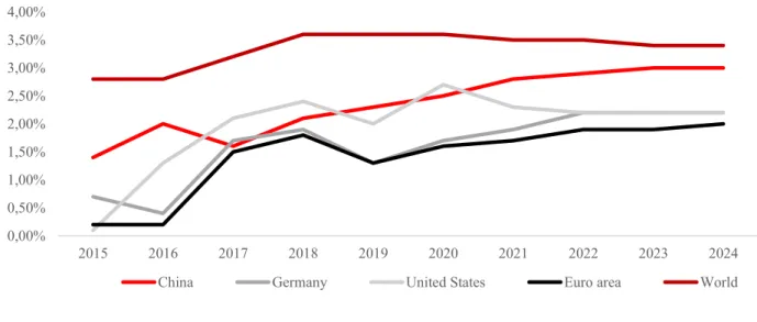
Figure 1 shows the forecasted growth rates for Hugo Boss’ main markets – Germany and the Euro area, USA and China – and the whole world (IMF, 2019a).

(27)

16 Figure 1: IMF GDP growth rates

Figure2 shows the current yield curves for the German Bund, US Treasury and the Chinese Government Bonds. Especially the flattening US yield curve fosters the remote growth outlooks since it is an indicator for a recession inferring the slowdown of economic growth (Reuters, 2019).

Figure 2: Current Yield Curves 0,00% 1,00% 2,00% 3,00% 4,00% 5,00% 6,00% 7,00% 8,00% 2015 2016 2017 2018 2019 2020 2021 2022 2023 2024

Real GDP growth, annual percentage

China Germany United States Euro area World

-1,00% 0,00% 1,00% 2,00% 3,00% 4,00% 5,00%

1MT 3MT 6MT 9MT 1YT 2YT 3YT 4YT 5YT 6YT 7YT 7YT 9YT 10YT 15YT 20YT 25YT 30YT

Yield Curves

(28)

17

Since I will forecast my sales in nominal values, the inflation rate of Germany is needed, in order to compute the nominal GDP. In order to give a fully outlook of inflation rates, the Chinese, US, world, and Euro area rates are also shown in figure 3 (IMF, 2019a).

Figure 3: Inflation Rates

3.2. Industry Outlook

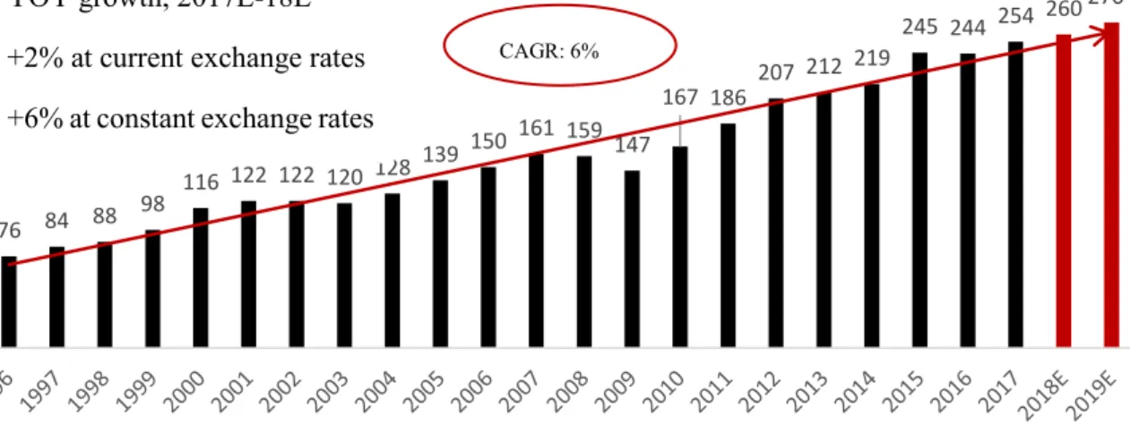
Most of 2018 was characterized by modest optimism within the apparel and luxury markets, resulting in a 6% growth and an estimated €260 billion in sales globally that were mainly driven by increasing local consumption (+4%). The generated sales through tourists remained flat on average (Bain & Company, 2019).

China was the main driver for the globally positive growth trend, which is reflected in an increase to 33% of the global total spendings in luxury goods in 2018, compared to 32% in 2017. Thus, China’s growth rate in 2018 was at 9%. The United States reached €80 billion, denoting a 5% growth rate that was fostered by a positive US economy. Due to a strong currency and limited tourists’ purchasing power, Europe fell back compared to the USA and China. However, local consumption was still positive, lifting retail sales up 3% to a total amount of €84 billion. Figure 4 shows the geographical distribution of sales growth expectations for the apparel industry (McKinsey & BoF, 2018):

0,00% 0,50% 1,00% 1,50% 2,00% 2,50% 3,00% 3,50% 4,00% 2015 2016 2017 2018 2019 2020 2021 2022 2023 2024

Inflation rate, annual change in percentage

(29)

18

Figure 4: Fashion Industry Sales Growth (McKinsey & BoF, 2018)

In contrast to the positive year of 2018, a potential shift in the global economic cycle causes uncertainty for the global economy in 2019 (McKinsey & BoF, 2018). Since the financial crisis in 2009 global growth has averaged about 2.5% per annum, but several signs indicate a decline or flattening in the upcoming years. The monetary policy of Federal Reserve started to raise interest rates again, increasing the cost of borrowing for companies. Furthermore, IMF and OECD forecast a flattening growth curve in developed countries (McKinsey & BoF, 2018). Therefore, the apparel industry will have to start focusing on cutting costs. They will most likely try to achieve that by organizational restructuring and end-to-end efficiency optimization. Despite the uncertainty in the short-term, a stable CAGR for 2018-2025 of 3-5% is expected, totaling in €320 - €365 billion (Bain & Company, 2019).

5 4 3 6,5 6 3 7,5 6 3,5 3,5 1,5 4,5 3 2 6,5 4 4.5 4.5 2.5 5.5 4 3 7.5 5 0 1 2 3 4 5 6 7 8 Total Fashion

Industry AmericaNorth Europemature emergingEurope Middle Eastand Africa Asia-Pacificmature Asia-Pacificemerging AmericaLatin

A nn ual gr ow th in %

Fashion industry sales-growth expectations 2018-19

(30)

19

3.3. Definition of Apparel and Luxury Goods Industry

The Apparel and Luxury Goods industry represents companies, that offer premium consumer goods like watches, clothes, jewelry or accessories (Bian & Forsythe, 2012). These products are highly desired due to the perception of prestige and high quality associated with them. Figure 6 shows the personal luxury goods segments and their sub-segments.Figure 6: Luxury personal goods segments (Statista 2019)

29% 27% 22% 15% 6% Luxury Apparel 21% Luxury Footwear 8% Luxury Watches 14% Luxury Jewelry 14% Prestige SKin Care

9% Prestige Cosmetics

8% Prestige Fragrances

5%

Luxury Personal Goods Segments

Luxury Fashion

Luxury Watches & Jewelry Prestige Cosmetics & Fragrances Luxury Leather Goods

Luxury Eyewear 76 84 88 98 116 122 122 120 128 139 150 161 159 147 167 186 207 212 219 245 244 254 260 270*

Personal Luxury Goods Market (€ billion)

YOY growth, 2017E-18E +2% at current exchange rates +6% at constant exchange rates

CAGR: 6%R

*Forecast for 2019 added by Denis Zimmerer based on historical CAGR of 6% Figure 5: Personal luxury goods industry (Bain & Company, 2019)

(31)

20

There is no exact definition of the Apparel and Luxury Goods industry, but most premium brands fulfill three characteristics that have psychological, pricing and quality effects (Husic & Cicic, 2009), (Vigneron & Johnson, 2004).

3.3.1. Psychological

The display of luxury goods gives consumers a feeling of power and confidence and the possibility to show their wealth and style in public. Therefore, persons who consume these goods are concerned about how they are perceived by others (Atwal & Williams, 2017).

3.3.2. Pricing

Apparel and luxury goods incorporate premium prices, which makes them more exclusive than other peer-products. Thus, they cannot be purchased by masses, since they have financial restrictions. Customers validate these high prices by the image of exclusivity and prestige, those products promise (Okonkwo, 2016).

3.3.3. Quality

Consumers expect a high quality product when purchasing luxury goods. High quality can be seen in the choice of materials, their durability or good craftmanship. Consumers are more willing to pay high prices if they are justified by high quality (Kapferer & Bastien, 2009)..

3.4. Industry Drivers

Several drivers for the apparel and luxury goods industry do exist. They are external factors that have an impact on the overall industry.

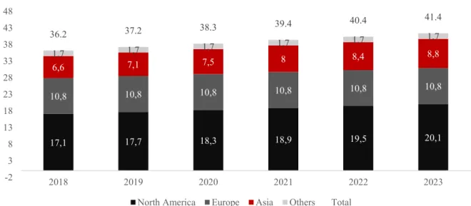
First, the global luxury goods market is driven by High Net Worth Individuals (HNWI) since they are able to afford the premium products. Hence, they are the target customers for apparel brands like Hugo Boss. Statista and Credit Swiss estimate that the number of HNWI will grow

(32)

21

to more than 41 million people by 2023 with Asia witnessing the highest increase, displayed in figure 7:

Figure 7: Forecasted Growth of HNWI (Statista 2019)

Secondly, 2017 approximately 31% of all luxury products were purchased while travelling due to a survey of Deloitte. Therefore, tourism – especially to Europe – affects the sales figures of apparel brands. Figure 8 shows a forecast for worldwide tourist arrivals by the World Tourism Organization, inferring that Europe will remain the most anticipated continent by tourists (Statista, 2019). 17,1 17,7 18,3 18,9 19,5 20,1 10,8 10,8 10,8 10,8 10,8 10,8 6,6 7,1 7,5 8 8,4 8,8 1,7 1,7 1,7 1,7 1,7 1,7 36.2 37.2 38.3 39.4 40.4 41.4 -2 3 8 13 18 23 28 33 38 43 48 2018 2019 2020 2021 2022 2023

Forecasted Growth of High Net Worth Individuals, in million

(33)

22 Figure 8: Forecast tourist arrivals (Statista, 2019)

3.5. Industry Trends

The apparel and luxury goods industry is facing several challenges and opportunities in the upcoming years. The biggest trends are a sales shift to emerging markets – especially China, digitalization, expansion of omnichannel presence and last but not least attracting millennials and generation z.

3.5.1. Sales Shift towards Emerging Markets

Historically, western markets were the most important ones for the luxury industry. However, recent years indicate that economic growth is shifting from the saturated western markets towards emerging markets in Asia and Latin America. Forecasts by McKinsey and Deloitte predict that by 2025 sales in emerging markets will be higher than in traditional western markets, as shown in figure 9 (Deloitte, 2017; McKinsey & BoF, 2017; McKinsey & BoF, 2018; Myers, 1974):

Figure 9:Global apparel and footwear sales forecast (McKinsey and BoF 2018)

134 135 137 138 139 140 570 576 581 586 590 594 290 295 300 305 309 312 221 223 224 226 227 228 1215 1229 1242 1254 1265 1274 2018 2019 2020 2021 2022 2023

Forecasted Tourist Arrivals, in million

(34)

23

The development of emerging markets contributes to a positive growth outlook for luxury companies. Especially in fast growing urban regions, upwardly mobile consumers demand more and more premium products instead of black market substitutes. However, many industry analysts contribute the shift towards emerging markets not only to the development of those countries, but also to the adoption of innovative retail concepts and business models (Deloitte, 2017). Moreover, the growth in emerging markets has been supported by optimizing the supply chain. Especially Chinese consumers will account approximately for 46% of the global apparel market by 2025, and their local consume will rise from currently 24% to 50% (Bain & Company, 2019). Furthermore India’s rapid growth in CAGR – shown in figure 10 – offers opportunities for apparel brands. Urban, upwardly mobile, tech-affine Indian millennials increase their demand for luxury products. However, the Indian market is still highly fragmented, which makes it difficult for apparel brands to establish successful strategies (McKinsey & BoF, 2018). In addition, luxury goods manufacturing countries increase their local consumption, whereas formerly the majority of goods were shipped to North America or Europe (McKinsey & BoF, 2017).

(35)

24

Figure 10: Real GDP CAGR forecast (McKinsey and BoF 2019)

3.5.2. Omni-Channel Presence and Distribution

Luxury apparel brands are late to adopt digitalization trends. The premium companies were reluctant to integrate e-commerce services in their distribution channels because they were afraid of jeopardizing their luxury image. Yet, nowadays customers expect a coherent customer experience across all channels – no matter if it is physically in a store or online (Deloitte, 2017). Thus, a challenge for the luxury market is to widen their channel presence and align the channels to fulfill the demand of unique customer experience (McKinsey & BoF, 2018).

Within the different channels of distribution wholesale remains the most dominant one which accounts for sales of 62% and growth of 1%. However, retail sales increased 4% throughout 2018, continuing the trend of apparel brands to control their customers in-store experience. A CAGR (2010-2018) of 9% for retail compared to 4% for wholesale underlines this development. Online sales persist to be the fastest growing channel, growing at 22% and reaching a market penetration of 10%. America contributed 44% to the total online sales, but growth was mainly due to Europe and China (Bain & Company, 2019). Figure 11 shows the sales by online channel, its YOY growth and the total market penetration of online sales.

1,5 2,3 3 3,7 6,1 8 Russia Brazil Mexico Turkey China India

(36)

25 Figure 11: Online sales (Bain & Company 2019)

3.5.3. New Generation

Millennials and generation z will represent between 40% - 50% of the overall luxury market until 2025 compared to 25% in 2016. Thus, millennials and generation z are driving growth in the upcoming years for apparel companies (Bain & Company, 2019; Deloitte, 2017). In fact, almost the whole market’s growth can be contributed to the new generation, compared with 85% in 2017. The new Generation differs to the previous in two fundamental aspects. They are digital pioneers and value driven consumers (McKinsey & BoF, 2018).

3.5.3.1. Digital Pioneers

First, they are digital pioneers who are more comfortable with new distribution channels like e-commerce or social media platforms. This has an impact on the fashion industry, since millennials are influenced by peer ratings, social media advertisement and influencers. Thus, they are more flexible to switch brands due to fashion trends and price sensitivity. Moreover, the new generation is more keen to purchase products online than any previous generation (McKinsey & BoF, 2017). This effect is displayed within the growth numbers of luxury online

1 1,3 1,9 2,3 2,6 3,3 4,3 5,5 7,4 9,3 11,3 14,9 17,9 22 26,8 1,00% 1,25%1,50% 1,75% 2% 2,50% 3% 3,50% 4% 5% 6% 7% 9% 10% 0% 1% 2% 3% 4% 5% 6% 7% 8% 9% 10% 0 5 10 15 20 25 30 35 40 2004 2005 2006 2007 2008 2009 2010 2011 2012 2013 2014 2015 2016 2017 2018E 25% 43% 21% 15% 27% 30% 28% 35% 26% 22% 32% 20% 23% 22% YOY Growth On lin e sales ( E UR b illi on )

Global personal luxury goods online sales (EUR billion)

Sales Online market penetration

(37)

26

shopping, which grew 22% in 2018 to $27 billion – representing 10% of all luxury sales. Therefore, one of the biggest challenges is developing smooth online services that simplify the purchase of goods. So far the luxury industry was reluctant to integrate online shopping into their business model, because they were afraid to damage their image of exclusivity (Deloitte, 2017). However, online-giants like Amazon or Alibaba accustom consumers to shorter delivery times and set new standards for online shopping. Luxury companies realized the importance of new distribution channels for the new generation and are now heavily investing into digitalization processes.

Nevertheless, millennials expect a holistic brand experience not only at the online platforms but also in physical stores (Deloitte, 2017). Therefore, the bar for customer satisfaction has been raised.

3.5.3.2. Value driven Consumers

The new generation consumes value driven. Companies in the luxury sector need to communicate their mission and practices in order to convince millennials from purchasing goods. Thus, the luxury sector has to pay attention to this new variable and align with its customers morals (McKinsey & BoF, 2017).

3.5.4. Design to Shelf

It is a competitive advantage for the apparel and luxury sector to have short “design to shelf”-time (McKinsey & BoF, 2017). This enables the companies to offer the latest fashion trends before the majority of the market. Moreover, it reduces store operating costs and excess inventory induced by fashion risk (McKinsey & BoF, 2017). New players are constantly accelerating the “design to shelf”-time, putting pressure on more traditional companies like Hugo Boss to optimize their supply chain. Furthermore, the new competitors already generate revenue mainly through new distribution channels like e-commerce or social media platforms, especially digital native companies like Alibaba or Amazon.

The digital shift is responsible for a steep decline of sales in traditional wholesale stores (McKinsey & BoF, 2017).

(38)

27 Figure 12: Average time to shelf (McKinsey and BoF 2018)

1 2 5 6 12 Missguided Boohoo Zara ASOS Traditional

(39)

28

4. Company Analysis

Equity valuations are only as strong as their underlying assumptions. Hence, its crucial to understand a company’s business in order to evaluate its up- and downsides as well as risks and chances accurately. Therefore, I am giving an overview of Hugo Boss’ mission and strategy, its past financial performance and a future outlook – concluding in a SWOT analysis to minimize distortions.

4.1. Company Overview

Hugo Boss is a German clothing company, dedicated to men’s and women’s premium apparel fashion and accessories. They develop, distribute and market their products internationally. It’s product portfolio consists of apparel, sportswear, shoes, accessories, fragrances, eyewear, watches, children’s fashion, home textiles and writing instruments. Hugo Boss markets two brands: BOSS and HUGO. BOSS focuses on business wear, leisure wear, watches, eyewear and fragrances, whereas HUGO contains more casual clothing like urban casual wear, sportswear, sneakers, children’s fashion or accessories (Reuters).

Hugo Boss currently employs 14.685 people in 129 countries, and accounts €2.8 billion sales generating an EBIT of €347 million in 2018. The company’s main distribution channel are its 1.113 own retail shops around the world, of which 585 are located in Europe.

The company is listed at Deutsche Börse’s XETRA with 69 mil. outstanding shares of which are 61.9 mil. free floating. Its shareholder structure is highly diversified with the Zignago Holding S.p.A. being the top investor with 7.1 mil. shares which account for 10.1% of Hugo Boss total shares. Hugo Boss is currently listed in the Mid-Cap-DAX (MDAX) which is Germany’s second biggest index behind DAX30, and consists of the 60 biggest companies according to market capitalization and volume behind DAX30.

4.2. Share Price Evolution

Hugo Boss was founded in 1924 by Hugo Ferdinand Boss. The company was first listed at 20 December 1985 issuing preferred shares. The first trading day for the ordinary shares was 22 May 1989. On 22 March 1999 Hugo Boss AG was initially included in the MDAX. The

(40)

29

preferred shares were replaced by ordinary shares in June 2012, when the share classes were merged (Hugo Boss, 2019b).

Around 88% of Hugo Boss’ shares are in free float and primarily held be institutional investors mainly from America and Europe. Due to a share buyback scheme from 2004 to 2007 Hugo Boss holds roughly 2% of its own shares. The biggest shareholders are Zignago Holding S.p.A. (10%), Black Rock Institutional Trust Company (5%) and Norges Bank Investment Management (3%). Thus, the strategic power is highly scattered between different shareholders (Hugo Boss, 2019b).

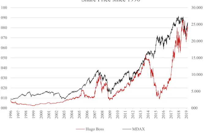
The performance of Hugo Boss’ share compared to its index can be seen in figure 13 (Reuters).

Figure 13: Share price development Hugo Boss and MDAX (Reuters)

Furthermore Hugo Boss’ relative return for the last 5 years compared to MDAX is shown in figure 14 (Reuters). It indicates, that Hugo Boss underperformed its benchmark index.

000 5.000 10.000 15.000 20.000 25.000 30.000 000 010 020 030 040 050 060 070 080 090 100 19 96 19 97 19 98 19 99 20 00 20 01 20 02 20 03 20 04 20 05 20 06 20 07 20 08 20 09 20 10 20 11 20 12 20 13 20 14 20 15 20 16 20 17 20 18 20 19

Share Price since 1996

(41)

30 Figure 14: Comparison Hugo Boss and MDAX

4.3. Hugo Boss Mission and Strategy

“We want to be the most desirable premium fashion and lifestyle brand globally.” (Hugo Boss,

2019a)

To achieve the above mentioned mission Hugo Boss AG announced the business plan until 2022 which will be presented in this chapter.

After the successful strategic merger of the brand’s BOSS Orange and BOSS Green into the brand HUGO, the company set two new main strategic goals until 2022. They want to personalize their products and increase the design to shelf speed through accelerating central processes. Simultaneously, the company wants to increase its profitability by growing sales 5-7% and EBIT to a 15% margin – which would beat the relevant market segment. The earnings growth shall result in expected free cash flows of between €250 million and €350 million per year in the coming years. Furthermore, improvements in the net working capital are planned – which would contribute to higher free cash flows. The free cash flow will mainly be used to fund dividend distribution. Through the healthy financial position and the ambitious growth outlook, Hugo Boss set a goal of distributing 80% of its free cash flow to its shareholders. Four factors will be crucial for Hugo Boss to accomplish this challenging goal. They want to grow their online business, improve the retail sales productivity, fully exploit the growth

0,30 0,50 0,70 0,90 1,10 1,30 1,50 1,70 M ai-2 01 4 Ju l-20 14 S ep -2 01 4 No v-2 01 4 Ja n-2 01 5 M rz -2 01 5 M ai-2 01 5 Ju l-20 15 S ep -2 01 5 No v-2 01 5 Ja n-2 01 6 M rz -2 01 6 M ai-2 01 6 Ju l-20 16 S ep -2 01 6 No v-2 01 6 Ja n-2 01 7 M rz -2 01 7 M ai-2 01 7 Ju l-20 17 S ep -2 01 7 No v-2 01 7 Ja n-2 01 8 M rz -2 01 8 M ai-2 01 8 Ju l-20 18 S ep -2 01 8 No v-2 01 8 Ja n-2 01 9 M rz -2 01 9 BOSS MDAX

(42)

31

potential in Asia, and an above average increase of sales of the newly formed brand HUGO in the contemporary fashion segment (Hugo Boss, 2019a).

4.4. Financial Performance

4.4.1. Historical Sales Performance

Hugo Boss currently sells its products in 129 countries. Their distribution activities are divided into three sales regions: Europe, Americas, and Asia. 63% of the total sales are generated within six core markets: Germany, USA, Great Britain, China, France and Benelux (Hugo Boss, 2019a).

Figure 15: Sales Distribution Hugo Boss (Hugo Boss, 2019a)

Hugo Boss’ main distribution channel is the groups own retail business which consists of directly operated stores, outlets and the online channel. Table 1 shows that sales grew throughout all distribution channels besides licenses. The increased distribution via online channels reflects Hugo Boss strategy to grow its e-commerce business and aligns with the industry trends mentioned in the previous chapter (Hugo Boss, 2019a).

Germany 15% Great Britain 13% France 6% Benelux 5% Other Europe 23% USA 15% Canada 3% Central & South

America 2% China 8% Oceania 2% Japan 2% Other Asian 3% Licences 3%

Sales Distribution

Europe, 63% Americas, 20% Asia, 15% Licences, 3%

(43)

32 Table 1: Sales by segment and Distribution Channels Hugo Boss

Explicit Period 1 2 3 4 5 6

Year 2014 2015 2016 2017 2018 2019E 2020E 2021E 2022E 2023E 2024E

Net sales (in EUR million) 2572 2809 2693 2733 2796 2872 2960 3058 3166 3278 3393

Growth 5.76% 9.21% -4.13% 1.49% 2.3% 2.70% 3.10% 3.30% 3.53% 3.52% 3.52%

Net sales by segments

Europe incl. Middle East and Africa 1,566 1683 1660 1681 1736 1776 1827 1883 1945 2010 2076

Europe (% of total) 60.89% 59.91% 61.64% 61.51% 62.09% 62% 62% 62% 61% 61% 61% Growth (in %) 7.48% 7.47% -1.37% 1.27% 3.27% 2.32% 2.83% 3.06% 3.33% 3.31% 3.30% Americas 587 671 582 577 574 583 592 602 613 625 637 Americas (% of total) 22.82% 23.89% 21.61% 21.11% 20.53% 20% 20% 20% 19% 19% 19% Growth (in %) 2.98% 14.31% -13.26% -0.86% -0.52% 1.50% 1.60% 1.73% 1.88% 1.88% 1.88% Asia/Pacific 361 393 382 396 410 434 461 490 522 555 590 Asia/Pacific (% of total) 14.04% 13.99% 14.18% 14.49% 14.66% 15.13% 16% 16% 16% 17% 17% Growth (in %) 4.03% 8.86% -2.80% 3.66% 3.54% 5.95% 6.20% 6.33% 6.40% 6.33% 6.26% Licenses 58 62 69 79 76 78 81 83 86 88 91 Licences (% of total) 2.26% 2.21% 2.56% 2.89% 2.72% 2.73% 2.72% 2.72% 2.70% 2.69% 2.67% Growth (in %) 0.00% 6.90% 11.29% 14.49% -3.80% 3.00% 3.00% 3.00% 3.00% 3.00% 3.00%

Net sales by distribution channel

Group's own retail business 1471 1689 1677 1732 1768 1844 1931 2026 2129 2237 2349

Retail (% of total) 57.19% 60.13% 62.27% 63.37% 63.23% 64.23% 65.23% 66.23% 67.23% 68.23% 69.23% Growth (in %) 14.82% -0.71% 3.28% 2.08% 4.33% 4.70% 4.89% 5.09% 5.06% 5.04% Wholesale 1043 1058 947 922 952 949 949 950 951 952 952 Wholesale (% of total) 40.55% 37.66% 35.17% 33.74% 34.05% 33.05% 32.05% 31.05% 30.05% 29.05% 28.05% Growth (in %) 1.44% -10.49% -2.64% 3.25% -0.31% -0.02% 0.08% 0.20% 0.08% -0.04% Licenses 58 62 69 79 76 78 81 83 86 88 91 Licences (% of total) 2.26% 2.21% 2.56% 2.89% 2.72% 2.73% 2.72% 2.72% 2.70% 2.69% 2.67% Growth (in %) 0.00% 6.90% 11.29% 14.49% -3.80% 3.00% 3.00% 3.00% 3.00% 3.00% 3.00%

SALES HUGO BOSS

(44)

33

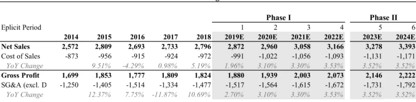
4.4.2. Historical Costs Performance

In 2018 selling and distribution expenses were below 2017 mainly due to a slowdown in retail expansion and positive effects from renegotiating rental contracts. Furthermore, marketing expenses decreased and expenses for logistics increased due to stronger performance of the online business. In addition, Hugo Boss limited the increase in administrative expenses, even though digital transformation processes were initiated (Hugo Boss, 2019a). Hugo Boss announced to decrease their COGS by up to 50 basispoints.

Table 2: Costs (Hugo Boss, 2019a)

4.4.3. Operating Results

Hugo Boss gross profit margin has been stable at 65% - 66% over the past 5 years. Nevertheless, its EBIT and adjusted EBITDA margins have both declined since 2014 due to the development of a new IT infrastructure for better online-distribution and the roll out of a new store concept for its retail stores (Hugo Boss, 2019b).

Eplicit Period 1 2 3 4 5 6

2014 2015 2016 2017 2018 2019E 2020E 2021E 2022E 2023E 2024E Net Sales 2,572 2,809 2,693 2,733 2,796 2,872 2,960 3,058 3,166 3,278 3,393 Cost of Sales -873 -956 -915 -924 -972 -991 -1,022 -1,056 -1,093 -1,131 -1,171

YoY Change 9.51% -4.29% 0.98% 5.19% 1.96% 3.10% 3.30% 3.53% 3.52% 3.52%

Gross Profit 1,699 1,853 1,777 1,809 1,824 1,880 1,939 2,003 2,073 2,146 2,222 SG&A (excl. DA) -1,250 -1,405 -1,514 -1,334 -1,477 -1,517 -1,564 -1,615 -1,672 -1,731 -1,792

YoY Change 12.37% 7.75% -11.87% 10.69% 2.70% 3.10% 3.30% 3.53% 3.52% 3.52%

Costs of Hugo Boss

Phase II Phase I

(45)

34 Figure 16: Operating Results (Hugo Boss, 2019a)

Hugo Boss’ EBITDA and EBIT margins are close to the industry average, which is probably a reason for the company’s efforts to increase their operating margins, even though they are already decent. (Statista, 2018)

4.4.4. Assets

Total assets rose 8% compared to 2017, which is mainly due to higher inventories and an increase in property, plant and equipment (PPE) and intangible assets. The share of current assets increased by 2% compared to the one of non-current through increased inventories that are aimed at supporting sales momentum in the group’s own retail business. Trade receivables and payables both increased at the same rate.

Other assets and liabilities did not significantly change compared to the previous year.

1699 1853 1777 1808 1824 1880 1939 2003 2073 2146 572 590 433 499 476 504 519 535 553 571 449 448 263 341 347 364 375 387 401 415 0% 10% 20% 30% 40% 50% 60% 70% 80% 90% 100% 0 500 1000 1500 2000 2500

2014 2015 2016 2017 2018 2019E 2020E 2021E 2022E 2023E

Operating Results, in million EUR

Gross profit EBITDA

EBIT Gross profit margin in %

(46)

35

4.5. Capital Structure

Hugo Boss book value of debt accounts for 47% of total assets as of 31 December 2018. Current and non-current financial liabilities account for 20% with a total book-value of €176 million. Furthermore the company has €147 million cash and cash equivalents at its disposal. Hugo Boss does not intend to change its capital structure.

4.6. SWOT Analysis

Figure 17: SWOT Analysis

Strength:

- Strong financial performance and margins enable Hugo Boss to further diversify its distribution channel and exploit online sales.

- The well established brand ensures Hugo Boss a loyal customer base that is willing to pay a higher premium for their products.

- Hugo Boss already has a strong

footprint in the uprising Asian markets, which gives it a heads up

position compared to competitiors.

Weaknesses:

- Declining sales in the wholesale

channel put pressure on the financial

performance.

- The main brand BOSS has a narrow

customer base which makes it

difficult to attract new customer segments.

- High Design-to-Shelf times comprise the risk of supplying the demanded products in time.

Opportunities:

- Growing demand in emerging

markets (especially China) presents

new sales opportunities for Hugo Boss.

- The new casual wear brand HUGO might unlock new customer segments.

Threats:

- Saturation in developed countries makes it difficult to increase and maintain the marketshare.

- Customer needs for ESG friendly products.

- Macroeconomic environment is dominated by uncertainty.

(47)

36

5. Valuation

In this section I will assess the fair value of Hugo Boss. My evaluation is mainly based on the DCF model which estimates the intrinsic value of the company. Furthermore, I will complement my findings with the relative valuation technique of the Multiples approach.

5.1. DCF Valuation

5.1.1. Free Cash Flows Projection

I expect Hugo Boss to reach a mature state in 2025. Therefore Free Cash Flows will be forecasted for 6 periods. In addition, the Terminal Value will be added. Furthermore, the FCF projections are split in three phases that will be explained in the next chapter. Towards the end of the explicit period my forecasted FCF aligns with Hugo Boss’ management announcement to generate €250 mil. to €350mil. FCF per year. However, reaching this FCF at the end of the explicit period reflects a more restrictive view compared to the management. The FCF is displayed in table 3. The complete DCF is shown in table 4.

Equity valuation of Hugo Boss AG