A Work Project, presented as part of the requirements for the Award of a Master Degree in Finance from the NOVA – School of Business and Economics.
The EU ETS: A Tale of Arbitrage Opportunities
Nuno Alexandre Tirapicos Dos Santos Reis, Nº 20329
A Project carried out on the Master in Finance Program, under the supervision of: João Pedro Pereira
The EU ETS: A Tale of Arbitrage Opportunities
1Nuno Alexandre Tirapicos Dos Santos Reis
Abstract
This work studies the presence of arbitrage opportunities following the announcements of the Market Stability Reserve of the EU ETS on May 2017, using the cost of carry model and three EUA futures contracts – December 2016, December 2017 and December 2018. The results suggest a long-run link between the spot and futures prices, but the cost of carry model does not explain well the price dynamics in the short run, which might be a sign for the presence of arbitrage opportunities in this market. These conclusions are especially important for European authorities, since they convey the inefficiency of the scheme.
Keywords: Energy Finance, European carbon market, European Union Emissions Trading Scheme
JEL Classification: G14, Q02, Q56
1Thanks are due to my advisor, João Pedro Pereira, for all the support and guidance; to professor Paulo M. M. Rodrigues for teaching Econometrics so clearly and with such passion and to my dear grandmother, for all the sacrifices she made to raise me.
1. Introduction
Climate change effects are nowadays a reality. The majority of the countries is starting to realise the pernicious effects pollution has on human health, on the environment and on the economy, either through direct or indirect channels. For that purpose, most of them signed and ratified the Kyoto Protocol, and more recently the Paris Agreement, in an attempt to mitigate the ecological footprint our actions have on the planet.
On these agreements, among other things, the participants committed themselves to reduce their greenhouse gas (GHG) emissions, by linking the multiple carbon emissions trading systems to avoid double counting, reporting regularly on their emissions and on their efforts to reduce them. Even though some large emitters have not ratified the Agreement – such as Russia, Turkey and Iran – and the US has shown their intention to withdraw, and therefore are not obliged to actively reduce their emissions’ levels through the establishment or the further development of their carbon trading systems, the emissions trading systems across the world transacted nearly US$82 billion in 2018 (World Bank Group, 2018), a 56% increase when compared with the 2017 level of US$52 billion (World Bank Group, 2017). The majority of this volume is attributed with the European Union’s Emissions Trading System (EU ETS), the first and the biggest major carbon market accounting for US$38 billion (Hodges, Krukowska and Carr, 2018) - 46% of the global market -, launched on the 1st of January 2005 as the major pillar of the European Union’s climate policy. After several years of low prices, this cap-and-trade system is finally starting to work the way it was intended, as the European regulators implemented some policies to deal with the undesirable excess of allowances, that accounted a total of 1.6 billion, on 12th May 2017 (European Commission, 2018).
The two main policies pursued by the regulators to deal with that issue were the backloading and the implementation of the Market Stability Reserve (MSR). The backloading was a short-term solution executed in February 2014, and consisted in the postponement of a total of 900
million allowances from 2014 to 2016, reducing the supply in each year, in an attempt to rebalance supply and demand and driving up the equilibrium prices, whereas the MSR is a long-term solution intended to stabilize the prices of the carbon allowances and will only start operating in January 2019. It works on the following way: If the total number of allowances in circulation exceeds the upper threshold of 833 million, a percentage of that excess is added to the reserve and stored, being released only when the total number of allowances in circulation is lower than the lower threshold of 400 million allowances. With this mechanism, the European authorities meant to drive up the prices of the allowances in the present, and decreasing them into the future, as the cap keeps diminishing, achieving this way a smoother path of prices.
Following the announcements of the European Parliament(2017) and of the Council of the European Union (2017), suggesting and adopting changes on the Market Stability Reserve, the market finally started to soar, after a prolonged slump: from approximately 5€ per tonne, the prices rose up to approximately 20€ per tonne, reaching 2009 values. This opportunity was only foreseen by some hedge funds and investment banks, which stuck with the sector even during its long slump, such as Goldman Sachs, JP Morgan and Morgan Stanley. However, some of the most successful winners were some relatively small hedge funds like Northlander Advisors, which was up 35,8% net of fees in August, and Lansdowne Partners Limited, which was up 11% by September, 2018 (Sheppard, 2018). This raises the question: Was this level of profits achieved by mere luck? Or are there persistent arbitrage opportunities related with market inefficiency?
The present work tries to study that, by using the cost-of-carry model to analyse the long-run link between the spot and futures prices of carbon, using econometric tools for that purpose. The existing literature is focused on two types of contracts: the intra-phase contracts, which are those that started and were completed within the same phase of the EU ETS, and the inter-phase ones, those which commenced and finished in different phases. That division is justified since
the pricing mechanisms and the relationships between the spot and the futures are different between the two types of contracts aforementioned, following the arguments found by Daskalakis, Phychoyios and Markellos (2009). Only the intra-phase contracts are considered here.
With respect to this specific type of contracts, the literature is ambiguous: Joyeux and Milunovich (2007, 2010) raised the possibility of arbitrage opportunities in the carbon market by proving that the futures contracts under analysis were not priced according to the cost-of-carry model, while Daskalakis, Phychoyios and Markellos (2009) showed that these contracts were well described by the cost-of-carry model with zero convenience yields. However, as suggested by Daskalakis and Markellos (2008), those profits could be explained by the immaturity of the market, since it was a recent market at that time, and by the restrictions on short-selling and banking European Allowances (EUA) from one phase to the next one, thus affecting the efficiency of the market. But from the literature under analysis to this date, several years have passed: the 3rd phase of EU ETS was initiated and, with it, some modifications described above – the MSR and backloading – were implemented. Therefore, some questions still remain: Did the 3rd phase and the introduction of the MSR increase market efficiency? What is behind the profits registered by some investment banks and hedge funds? Higher returns associated with a higher level of risk, or arbitrage opportunities? These are the questions this work tries to answer.
This thesis is organized as follows: Part 2 presents the econometric model used. Part 3 introduces the dataset used for the purpose of this analysis and the unit root tests, as well as some descriptive statistics of the series. Part 4 studies the long-run relationship between the spot and the futures prices series selected. Part 5 examines the presence, or not, of arbitrage opportunities, using the cost-of-carry model. Part 6 concludes the thesis.
2. Econometric Model
The cost of carry model represents the net cost of holding an investment position, and is generally used for the pricing of futures contracts. It expresses the relationship between the futures and spot prices, compounded by the cost of carry, which, in turn, can encompass the risk-free interest rate, the convenience yield (in case of a commodity), the dividend yield (in case of stocks paying dividends), storage/transportation costs, and the time to delivery of the
contract. This relationship can be summarized by the following equation:
Ft,T = St e(rf + u – y) * (T – t) (1)
being Ft,T the actual price of a futures contract expiring in T-t years, St the prevailing spot price,
rf the discount rate, u the storage/transportation cost and y the convenience/dividend yield. The
no arbitrage condition required by the model implies that the risk-free rate is the appropriate discount rate to be used (Hull, 2008).
In the specific case of the EU ETS, the storage/transportation costs are not really a concern – they are at most documents – as well as the dividend yield/convenience yield – firstly because the emission allowances do not pay any dividends, and secondly because the carbon emitters are not required to constantly hold spot allowances. The only time they are required to hold those allowances are at the time they must settle their carbon accounts.
Therefore, the cost of carry model is simplified to the following:
Ft,T = St e rf * (T – t) (2)
Theoretically, and in a perfect market without frictions, the aforementioned condition should always apply at any time. Nonetheless, given the presence of imperfections such as restrictions on short-selling, transactions costs, asymmetric information, among others, this
condition might not apply and differences between the theoretical price and the traded price are bound to arise, especially in the short-run (Mackinlay and Ramaswamy, 1988).
By taking natural logarithms in both sides of the previous equation, we were able to simplify the cost of carry model:
ln[Ft,T ]= ln [St e rf * (T – t)] ⬄
ln[Ft,T ]= ln [St]+ln[e rf * (T – t)] ⬄
ft= st + rf(T-t)*ln[e]
With the transformations previously applied, we were able to achieve a long-run cointegrating equation:
ft= st + rf(T-t)+ vt (3)
being st≡ ln[St], ft ≡ ln[Ft] and vt a disturbance term. (T-t) is the reverse time trend that initiates
at T – the maturity of the contract – and converges to zero as t approaches T.
To evaluate the validity of the cost of carry model, we reformulate the cointegrating equation as follows:
ft = αst + β[rf(T-t)]+ vt (4)
Two types of hypothesis were considered at this stage:
➢ H0: vt is stationary, this is, the equation above-mentioned exhibits a cointegration relationship;
➢ H0: α = β = 1 this is, the constraints implied by the cost of carry model hold. The interpretation of the previous hypothesis has the following meaning:
If the equation exhibits a cointegration relationship and the restrictions implied by the cost of carry hold, that would imply that there is a long-run relationship between the spot prices, the futures prices and the risk-free rate, in accordance with the cost of carry model. Moreover, that would also imply the efficiency of the carbon futures market, in a manner that the cost of carry model explains well the price dynamics in the short run and so it is not expected arbitrage
opportunities to show up between holding futures contracts or spot instruments carried until maturity at the risk-free rate.
For its turn, if the equation exhibits a cointegration relationship but the restrictions implied by the cost of carry model do not hold, that would imply that the long-run link would still be viable – this is, the series move together in the long-run; however, that relationship is not given by the cost of carry model in the short run, and therefore it would not be strange if arbitrage opportunities appear in the carbon market. The restrictions implied by the cost of carry model stem from the definition of market efficiency: according to Fama (1970), an efficient market in its weak form would imply that the changes on prices from one period to the next should be unpredictable.
The last scenario is achieved if the equation does not exhibit a cointegration relationship and the restriction implied by the cost of carry model do not apply as well. In such scenario, not only the futures price is disentangled from the spot prices, meaning their paths are completely independent of each other, but would again point out the possibility for arbitrage opportunities to be persistent in this market or that the price dynamics in this market are not explained by the cost of carry model, which confirms the conclusions of Joyeux and Milunovich (2007, 2010).
By looking at the literature, we can find examples of the application of this econometric approach in several financial markets, whether in commodities such as oil, or in equity markets. For instance, Wahab and Lashgari (1993) shown that the spot and futures prices for both the S&P 500 and the FTSE 100 were cointegrated, meaning there is a long-run link between the two markets and they trend together, a conclusion in accordance with market efficiency. Passing on to commodities, which should be the focus of the literature review since the allowances of the EU ETS are considered themselves a commodity, we found more support to our model: Zapata and Fortenbery (1996) proved the joint cointegration of futures and spot prices as well
as the interest rates of Chicago corn and soybean market; for its turn, Yang, Bessler and Leatham (2001) tested the cointegration of US agricultural commodity futures and spot markets, indicating that not even the asset storability affected that long-run relationship, putting in question works of previous authors (Covey and Bessler, 1995). Lastly, in the oil commodity market, Crowder and Hamed (1993) also used a cointegration analysis to study the relationship between the spot and futures in this market, while Lee and Zeng (2011) applied a new method of quantile cointegrating regressions to examine the relationship of spot and futures oil markets of West Texas Intermediate, corroborating one more time the long-run link between the two series, although with a caveat: the length of the future contract has an impact on the cointegrating relationship between the futures and the spot oil prices.
3. Dataset, Descriptive Statistics & Unit Root Tests
The dataset consists on daily observations of carbon spot prices, two interest rate variables – the 1 month and 3 months Euribor – and carbon futures prices of the December 2016, December 2017 and December 2018 contracts, over the period ranging from 02/05/2016 to 31/10/2018.
All the series were collected from DataStream, although the spot and futures carbon prices refer to the settlement prices of the European Energy Exchange (EEX). A graph with the spot and carbon prices is presented next:
Source: Authors’ construction. Based on the information gathered on DataStream.
By the simple observation of the graph, some features stand out: the four series move in close relation to each other and in the same direction – in fact, their relationship is so close that the series overlap each other. While in the beginning they do not seem to have an upward or downward trend, that fact appears to have changed from the second trimester of 2017 onwards. This increase in prices is consistent with the announcement of the European Commission on the 12th of May 2017, on which they published for the first time the number of carbon allowances in circulation. That number plays a very important role for the functioning of the MSR, by allowing the investors to know exactly how many allowances are going to be stored in the reserve or released from it, helping in the forecast of the prices.
The next step would be to analyse some descriptive statistics of the series, to understand their properties:
Table 1: Descriptive statistics of EUA spot and futures prices and short-term Euribor
Table 1 presents us some interesting insights. The first thing to be stressed out is the daily standard deviation of the prices – from a very low value in the beginning of the sample, we can see it increase, especially in the spot and in the 2018 futures contract, which captures the remarkable increase of the prices of allowances; the kurtosis and skewness coefficients of the returns suggest a leptokurtic and positive skewed distribution for the 2016 and 2017 contracts and a leptokurtic and negative skewed distribution of the spot and the 2018 futures series – which indicates that, in the first two contracts, there is a higher frequency of outcomes in the tails of the distribution, although with a higher change of extremely positive outcomes, whereas in the last two the higher frequency of outcomes in tails also holds, but now with a higher change of extremely negative outcomes. This is consistent with historical returns of financial assets, which usually show little evidence of skewness but high evidence of excess kurtosis (Campbell, Lo and MacKinley, 1997).
The Jarque-Bera test (Jarque and Bera, 1987) uses the previous results of skewness and kurtosis to test whether the underlying distribution of a series is normal or not. In case of rejection of the null hypothesis indicates that the underlying distribution is not normal; in the
Eur1m Eur3m
Prices Log Ret Prices Log Ret Prices Log Ret Prices Log Ret Eur1m Eur3m
# Obs 166 165 426 425 653 652 653 652 653 653 Mean 5,184 -0,0011 5,5603 0,0004 8,7515 0,0015 8,6957 0,0015 -0,3698 -0,318 Median 4,975 -0,0016 5,275 0 6,15 0,0018 6,07 0,0017 -0,371 -0,327 Maximum 6,51 0,1085 7,92 0,1241 25,24 0,123 25,19 0,1263 -0,343 -0,25 Minimum 3,91 -0,1282 3,94 -0,127 3,99 -0,1941 3,91 -0,1945 -0,375 -0,332 Std. Dev 0,6886 0,0341 0,9584 0,0324 5,081 0,0309 5,0916 0,0308 0,00527 0,018 Skewness 0,0434 0,1378 0,7921 0,085 1,2579 -0,3778 1,2541 -0,3805 3,199 2,1171 Kurtosis 1,5908 3,8002 2,6475 4,9898 3,3073 6,589 3,2961 6,6941 13,1367 7,0221 Jarque-Bera 13,7875* 4,9251 46,7493* 70,6249* 174,7656* 365,4529* 173,5606* 386,4687* 3910,143* 927,9421*
Note: One star indicates significance at 5% level;
Prices refers to daily closing price, and Log Ret refers to logarithmic returns
series under analysis, only the returns of the 2016 futures contract seem to have a normal distribution at a 5% confidence level, while for the others, both at levels and returns, the normal is clearly rejected.
Before going to the cointegration, one earlier step is required: to assess the stationarity of each individual series using unit root tests (Mills and Markellos, 2008). However, since one of the usual problems with this type of tests is the existence of structural breaks of the series, which reduces their power, we decided to apply the usual Augmented Dickey-Fuller (ADF) test (Dickey and Fuller, 1979, and Said and Dickey, 1984) jointly with a unit root test which allows for a structural break (Vogelsang and Perron, 1998) to evaluate the differences in conclusions between the two. If the conclusions are different, it would be a signal for the presence of a structural break.
The following table resumes the both unit root tests employed on the logarithmic spot and futures series, as well as in the interest rate series:
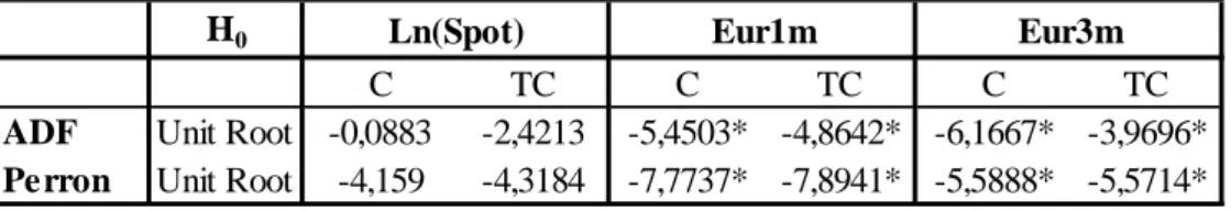
Table 2: Unit root tests H0
C TC C TC C TC
ADF Unit Root -0,0883 -2,4213 -5,4503* -4,8642* -6,1667* -3,9696*
Perron Unit Root -4,159 -4,3184 -7,7737* -7,8941* -5,5888* -5,5714* Note: One star indicates significance at 5% level
C refers to the unit root test only with constant, and TC refers to the unit root test with trend and constant
Ln(Spot) Eur1m Eur3m
H0
C TC C TC C TC
ADF Unit Root -1,8952 -1,788 -1,6822 -2,5586 -0,0998 -2,446
Perron Unit Root -3,963 -3,7577 -4,1273 -4,261 -4,2021 -4,3144 Note: One star indicates significance at 5% level
C refers to the unit root test only with constant, and TC refers to the unit root test with trend and constant
Table 2 concludes that both tests yield the same conclusions. The null of an existing unit root is accepted on levels for the spot and for all the futures series while it is rejected for the interest rate series – this means that logarithmic spot and futures are not stationary, whereas the interest rates are. The null is only rejected – and so stationarity is achieved - by applying first differences to the logarithms of spot and futures, which specifies that those series are integrated of order 1 – I(1) – while the interest rates are integrated of order 0 – I(0).
Since the conclusions of both the ADF test and the unit root test with a structural break are the same, that means that our series do not have structural breaks, a feature that simplifies the analysis. This conclusion is consistent with the visual inspection of Figure 1, in which we do not observe the existence of structural breaks.
4. Cointegration Analysis
Having fulfilled the requirements needed to perform the cointegration analysis – the identification of the order of integration of the series – we proceed with the cointegration tests. For this purpose, the selected model was the one proposed by Engle and Granger (1987). The interest rates were left out of the cointegrating regression since the aforementioned model requires all variables to be integrated or order 1, which is opposite to the order of integration of the interest rates. Thus, the potential cointegrating regression would be:
st = θ0 + θ1 ft + zt (5)
In this case, the cointegration is verified if the residuals of the cointegrating regression are integrated of order 0. The following table summarizes the results of the regression:
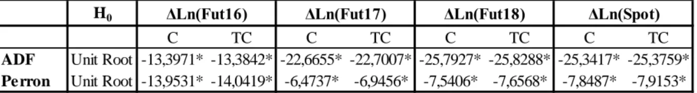
H0
C TC C TC C TC C TC
ADF Unit Root -13,3971* -13,3842* -22,6655* -22,7007* -25,7927* -25,8288* -25,3417* -25,3759*
Perron Unit Root -13,9531* -14,0419* -6,4737* -6,9456* -7,5406* -7,6568* -7,8487* -7,9153* Note: One star indicates significance at 5% level
C refers to the unit root test only with constant, and TC refers to the unit root test with trend and constant
ΔLn(Spot)
Table 3: Cointegration Analysis
This time only the ADF test was applied, since we already proved that structural breaks are not an issue of our model; therefore, the Perron test with a structural break is not used.
The conclusion is as expected: Since we reject the null hypothesis of a unit root, we can argue that the residuals of the cointegrating regressions of the three futures prices are integrated of order 0, so stationary. The implication of this result follows the same conclusions of the authors previously mentioned: There is a long-run relationship between the spot and the futures series consistent with the cost of carry model.
5. Arbitrage opportunities using the cost of carry model
Having proved one of the hypothesis of this paper, we pass now to the other: assessing if the restrictions implied by the cost of carry model hold, so that we could understand the presence of arbitrage opportunities in the short-run.
The tables below have the summary of the cointegrating regression and the joint significance test under analysis:
Table 4: Cointegration regression estimation
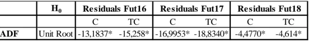
H0
C TC C TC C TC
ADF Unit Root -13,1837* -15,258* -16,9953* -18,8340* -4,4770* -4,614*
Note: One star indicates significance at 5% level
C refers to the unit root test only with constant, and TC refers to the unit root test with trend and constant
Residuals Fut16 Residuals Fut17 Residuals Fut18
Fut16 Fut17 Fut18
α 0,999 1,000 1,000
(0,003) (0,002) (0,001)
β -0,003 -0,006 -0,008
(0,002) (0,001) (0,0004)
Note: The values without brackers refer to the estimators of the parameters α and β and the values in brackers are the standard errors associated with the estimators.
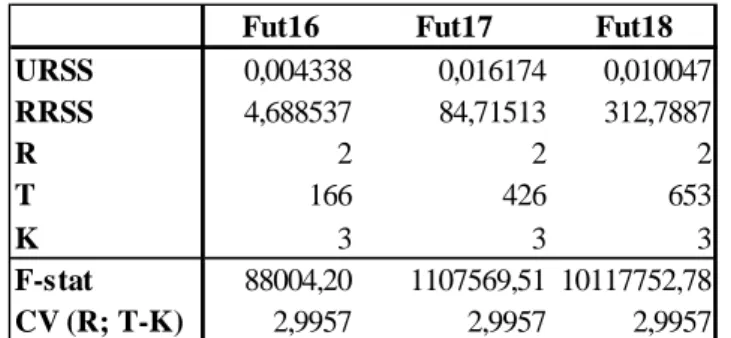
Table 5: Joint significance tests
On Table 5, we can see that the estimator of α, the parameter associated with the spot carbon price, is very close to its theoretical value, in the three contracts considered.
For its turn, Table 6 presents us the F-test conducted on the restrictions imposed on α and β. Since the F-test values are higher than the critical values for each contract, this means that we reject the null hypothesis of α = β = 1. Therefore, since the three contracts are cointegrated and show linkages in the long-run, but the restrictions implied by the cost of carry model do not hold, that means that the short run price dynamics in this market are not explained by the cost of carry model with zero convenience yield, and so this market might not be efficient, in its weakest form.
6. Conclusions
We investigated the presence of arbitrage opportunities and market efficiency in the EU ETS following news of unusual levels of profits for this type of securities, after announcements of the functioning of the Market Stability Reserve on May 2017.
For this purpose, the cost of carry model was tested using three EUA futures contracts – December 2016, December 2017 and December 2018. The cointegration analysis revealed that all the contracts maintain a long-run relationship between the futures and the spot prices, while the joint hypothesis of the coefficients associated with the spot prices and the interest rates
Fut16 Fut17 Fut18
URSS 0,004338 0,016174 0,010047 RRSS 4,688537 84,71513 312,7887 R 2 2 2 T 166 426 653 K 3 3 3 F-stat 88004,20 1107569,51 10117752,78 CV (R; T-K) 2,9957 2,9957 2,9957
Note: URSS refers to Unrestricted Residual Sum of Squares, RRSS to Restricted Residual Sum of Squares, R to the number of restrictions, T to the number of observations, K to the number of regressors plus the constant and CV (R; T-K) to the critical value for the F-distribution with R number of regressors and T-K degrees of freedom.
being equal to one was clearly rejected by the tests considered, meaning that or the cost of carry model with zero convenience yield does not explain well the price dynamics in this market, or the market is not efficient in its weakest form, and therefore persistent arbitrage opportunities are likely to occur.
Although these conclusions appear to be consistent with the recent news conveyed by financial newspapers, shedding some light about the market inefficiency of the EU ETS, there is scope for improvement: the Market Stability Reserve will only start operating in 2019 and the expectations regarding its functioning might not correspond to the reality; in fact, the rise in prices and the excitement shown by investors might be a self-fulfilling prophecy. Further research should focus on the post-implementation of the MSR, especially after the announcements released by the European institutions of the 1st year of functioning of this new mechanism.
Apart from the functioning of the MSR, there are still other limitations of the system under analysis. The first studies about the efficiency of the EU ETS (Milunovich and Joyeux, 2007; Daskalakis and Markellos, 2008) had the same conclusion: the behaviour of the EU ETS is not compatible with the weak form of efficiency. If some of the arguments presented by the authors were related to the recent birth of the market, the same type of argument is not applicable nowadays: almost 15 years have passed since the beginning of the market, and apparently it is still not efficient. However, one important argument used to justify this apparent inefficiency is still valid: the impossibility to short sell the allowances is one of the factors pointed out by the authors of the aforementioned studies. Therefore, further studies should be conducted on the reasons behind this inefficiency, to assess if it is due to the design of the European carbon system.
Other limitation could be attributed to the model used in this thesis, especially to the assumption made on the convenience yield term. Instead of assuming a value of zero, we could
simply assume the convenience yield term to be positive: if, when required to settle their carbon accounts, the carbon emitters do not have the number of allowances corresponding to the amount of emissions released, they are required to pay a fine of 100 € per tonne of CO2 for which they have no allowances; in consequence, there might be a premium connected with holding the allowances until the settlement date. Even so, we considered that convenience yield to be negligible, given that there is a 1.6 billion excess of carbon allowances on the market, making the probability of not finding allowances in the market in the time of the settlement date very close to 0. Nonetheless, with the introduction of the MSR the number of excess allowances will decrease, possibly increasing the premium related with holding the allowances until the settlement date, making it different from zero. Studies should be performed on the effectiveness of the cost of carry model with a positive convenience yield to explain the price dynamics in this market, possibly testing other alternative models to capture the price dynamics observed.
Lastly, the scope of this analysis was only intra-phase futures contracts. As also shown by some authors (Daskalakis, Psychoyios and Markellos, 2009), there are significant differences in the pricing of intra and inter-phase contracts. Since inter-phase contracts were not considered, an interesting object of study would be the analysis of arbitrage opportunities in both types of contracts.
References
[1] Campbell, John Y., Lo, Andrew Y., A. Craig MacKinley. 1997. The Econometrics of Financial
Markets. New Jersey: Princeton University Press.
[2] Council of the European Union. 2017. “Proposal for a Directive of the European Parliament and of the Council amending Directive 2003/87/EC to enhance cost-effective emission reductions and
low-carbon investments”. Accessed November 20th.
http://data.consilium.europa.eu/doc/document/ST-6841-2017-INIT/en/pdf
[3] Covey, Ted and David A. Bessler. 1995. “Asset storability and the information content of intertemporal prices.” Journal of Empirical Finance, 2(2): 103-115.
[4] Crowder, William J., and Anas Hamed. 1993. “A cointegration test for oil futures market efficiency.”
[5] Daskalakis, George and Raphael N. Markellos. 2008. “Are European Carbon Markets Efficient?.”
Review of Futures Markets, 17 (2): 103-128.
[6] Daskalakis, George; Psychoyios, Dimitris and Raphael N. Markellos. 2009. “Modeling CO2 emission allowances prices and derivatives: Evidence from the European trading scheme.”
Journal of Banking and Finance, 33: 1230-1241.
[7] Dickey, David A.. and Wayne A. Fuller. 1979. “Distribution of the Estimators for Autoregressive Time Series With a Unit Root.” Journal of the American Statistical Association, 74(366): 427-431.
[8] Engle, Robert F., and Clive W. J. Granger. 1987. “Co-Integration and Error Correction: Representation, Estimation, and Testing.” Econometrika, 55 (2): 251-276.
[9] European Commission. 2017. “Commission publishes first surplus indicator for ETS Market Stability Reserve”. Accessed December 2nd.
https://ec.europa.eu/clima/news/commission-publishes-first-surplus-indicator-ets-market-stability-reserve_en
[10] European Commission. 2018. “Communication from the Commission: Publication of the total number of allowances in circulation in 2017 for the purposes of the Market Stability Reserve under the EU Emissions Trading System established by Directive 2003/87/EC”. Accessed
November 20th.
https://ec.europa.eu/clima/sites/clima/files/ets/reform/docs/c_2018_2801_en.pdf
[11] European Parliament. 2017. “Amendments adopted by the European Parliament on 15 February 2017 on the proposal for a directive of the European Parliament and of the Council amending Directive 2003/87/EC to enhance cost-effective emission reductions and low-carbon
investments”. Accessed November 20th.
http://www.europarl.europa.eu/sides/getDoc.do?pubRef=-//EP//TEXT+TA+P8-TA-2017-0035+0+DOC+XML+V0//EN
[12] Fama, Eugene F. 1970. “Efficient Capital Markets: A Review of Theory and Empirical Work.” The Journal of Finance, 25(2): 383-417.
[13] Hodges, Jeremy; Krukowska, Ewa and Mathew Carr. 2018. “Europe's $38 Billion Carbon Market
Is Finally Doing Its Job.” Bloomberg, March 26.
https://www.bloomberg.com/news/articles/2018-03-26/europe-s-38-billion-carbon-market-is-finally-starting-to-work
[14] Hull, John C. 2008. Options, Futures and Other Derivatives. Upper Saddle River: Prentice Hall. [15] Jarque, Carlos M., and Anil K. Bera. 1987. “A Test for Normality of Observations and Regression
Residuals.” International Statistical Review, 55(2): 163-172.
[16] Joyeux, Roselyne and George Milunovich. 2010. “Testing market efficiency in the EU carbon futures market.” Applied Financial Economics, 20: 803-809.
[17] Lee, Chien-Chiang and Jhih-Hong Zeng. 2011. “Revisiting the relationship between spot and futures oil prices: Evidence from quantile cointegrating regression.” Energy Economics, 33(5): 924-935.
[18] Mackinlay, A. Craig and Krishna Ramaswamy. 1988. “Index-Futures Arbitrage and the Behavior of Stock Index Futures Prices.” The Review of Financial Studies, 1 (2): 137-158.
[19] Mills, Terrence C., and Raphael N. Markellos. 2008. The Econometric Modelling of Financial Time
Series. New York: Cambridge University Press.
[20] Milunovich, George and Roselyne Joyeux. 2007. “Pricing Efficiency and Arbitrage in the EU ETS Carbon Futures Market.” Journal of Investment Strategy, 2 (2): 23-25.
[21] Said, Said E., and David A. Dickey. 1984. “Testing for Unit Roots in Autoregressive-Moving Average Models of Unknown Order.” Biometrika, 71(3): 599-607.
[22] Sheppard, David. 2018. “Hedge funds and Wall St banks cash in on carbon market’s revival.”
Financial Times, September 7.
https://www.ft.com/content/6e60b6ec-b10b-11e8-99ca-68cf89602132
[23] Vogelsang, Timothy J., and Pierre Perron. 1998. “Additional Tests for a Unit Root Allowing for a Break in the Trend Function at an Unknown Time.” International Economic Review, 39(4): 1073–1100.
[24] Wahab, Mahmoud and Malek Lashgari. 1993. “Price Dynamics and Error Correction in Stock Index and Stock Index Futures Markets: A Cointegration Approach.” Journal of Futures Markets, 13 (7): 711-742.
[25] World Bank Group. 2017. “State and Trends of Carbon Pricing 2017”. Accessed November 20th.
http://documents.worldbank.org/curated/en/468881509601753549/State-and-trends-of-carbon-pricing-2017
[26] World Bank Group. 2018. “State and Trends of Carbon Pricing 2018”. Accessed November 20th.
https://openknowledge.worldbank.org/bitstream/handle/10986/29687/9781464812927.pdf?seq uence=5&isAllowed=y
[27] Yang, Jian; Bessler, David A. and David J. Leatham. 2001. “Asset Storability and Price Discovery in Commodity Futures Markets: A New Look.” Journal of Futures Markets, 21(3): 279-300. [28] Zapata, Hector O., and T. Randall Fortenbery. 1996. “Stochastic Interest Rates and Price Discovery