DURATION OF WEATHERING EPISODES IN SMALL WATERSHEDS: IMPLICATION ON PLAGIOCLASE WEATHERING RATES
Pacheco FAL1, Medina, J2, Ribeiro, S2, Van der Weijden CH3
1Department of Geology and Centre for Chemistry, Trás-os-Montes and Alto Douro University, Ap. 1013, 5000
Vila Real, Portugal, [email protected].
2University of Aveiro 3810-193 Aveiro, Portugal, [email protected], [email protected]
3Department of Earth Sciences—Geochemistry, Faculty of Geosciences, Utrecht University, P.O. Box 80.021
3508 TA Utrecht, The Netherlands, [email protected].
Abstract
Spring watersheds were characterized for their morphological and hydrographical parameters using GIS, and depths of spring water circulation were determined using correlations between depths of conductive fractures measured in drilled wells and concomitant 87Sr/86Sr ratios in drilled well waters. Subsequently, mathematical
approaches were used to estimate aquifer’s hydraulic conductivities and effective porosities, and groundwater travel times, from measured spring discharge rates. Finally, a mole balance model was used to derive the relevant weathering reactions contributing to spring water composition. Combining all this data, plagioclase weathering rates could be calculated for each spring site and checked against literature results. Notwithstanding natural weathering is operating over geological time scales, the calculated rates follow the trend of experimental results that work on fresh materials, suggesting that current weathering episodes operating within the watersheds are not far from their starts. Different results are obtained when the analysis is focused on soil profiles.
Key-words: spring watershed, soil profile, plagioclase weathering rate, groundwater travel time.
Resumo
Bacias hidrográficas de nascentes foram caracterizadas relativamente aos seus parâmetros morfológicos e hidrográficos usando SIG, e as profundidades de circulação das águas de nascente foram determinadas utilizando correlações entre profundidades de fracturas condutoras medidas em furos e as razões 87Sr/86Sr das suas águas.
Subsequentemente, aproximações matemáticas foram usadas para estimar condutividades hidráulicas e porosidades efectivas do aquífero fracturado, assim como tempos de circulação da água subterrânea, a partir dos registos de descarga das nascentes. Finalmente, um modelo de balanço de massa foi usado para derivar as reacções de alteração relevantes que determinaram a composição química das nascentes. Combinando todos estes dados foi possível calcular taxas de alteração da plagioclase para cada nascente e comparar os resultados com a literatura publicada. Não obstante a alteração natural ao nível das bacias hidrográficas operar continuamente ao longo dos tempos geológicos, as taxas calculadas seguem a tendência observada em trabalhos experimentais que lidam com materiais frescos, sugerindo que os episódios de alteração correntes não estão longe do seu início. Resultados diferentes obtêm-se quando a análise incide sobre perfis de alteração de solos.
Palavras-chave: bacia hidrográfica de nascente, perfil de alteração, taxa de alteração da plagioclase, tempo de
percurso da água subterrânea.
1. Introduction
Weathering is a multi-scale and multi-stage process, whereby a fresh rock is converted into disaggregated plasma, and rates of mineral weathering determined by various methods reflect the differences in the temporal and geometric scales on which the approaches are standing. This paper is a contribution for the understanding of the weathering process of plagioclase at the spring watershed scale.
2. Study Area
The region of Vila Pouca de Aguiar is located in the North of Portugal and occupies an area of approximately 437 km2. The geology of the area is characterized by Hercynian (syn- to post-tectonic) granites that intruded Palaeozoic (Cambrian to Devonian) metassediments and were covered by Quaternary alluvial and terrace deposits along a large-scale tectonic structure known as the Vila Real fault. The Vila Pouca de Aguiar granites are composed of quartz (31.5%), plagioclase (35.3), K-feldspar (26.7), biotite (4.4) and muscovite (1.4), with minor amounts of apatite and ilmenite. The plagioclase composition ranges from albite-An8 to
andesine-An37 (Pacheco et al., 1999). The metassediments, which include greywackes,
phyllites, quartzites and graphitic slates, contain quartz, muscovite and smaller amounts of biotite, K-feldspar and albite-oligoclase (Pacheco, 1995). Climate in the area is temperate with wet-cold and dry-warm alternating seasons. The annual precipitations range from 900 mm/y in the Northeast to 1900 mm/y in the Southwest of the region (Figure 1).
Figure 1 – Location and simplified geologic map of the Vila Pouca de Aguiar region. Distribution of the annual precipitation (contours), and of sampled drilled wells and springs. The labels close to the sampling sites are in agreement with the Nr codes in Tables 1a and 1b.
3. Borehole and Spring Water Chemistry
Samples of granite and metassediment springs were collected within the limits of the Vila Pouca de Aguiar municipality, in July–November 2007 for chemical analysis of major dissolved compounds and strontium, and in November 2007–June 2008 for isotopic analysis of strontium (87Sr/86Sr). Drilled well and rainwater samples were collected in October– December 2008 and January 2009, respectively, for analysis of 87Sr/86Sr. The sampling sites are shown in Figure 1. At the sampling site, a water sample was collected and filtered through a 0.4 μm membrane filter. The filtered water was split into 4 portions: portions 1 and 2 were stored for chemical analysis at the laboratories of the Earth Sciences—Geochemistry department of the Utrecht University (The Netherlands), the first acidified with HNO3 until
pH ≤ 2; portion 3 was stored for isotopic analysis of strontium at the laboratory of isotope geology of the Aveiro University (Portugal), also acidified with HNO3 until pH ≤ 2; and
portion 4 was stored for analysis of alkalinity in the field laboratory, within 24 hours using the Gran plot method. Sodium, potassium, magnesium, calcium, and silicon were analyzed by ICP-OES in portion 1, while chloride, sulfate, and nitrate were determined by ion chromatography in portion 2. Approximately 50 ml of portion 3 were evaporated and the final residues were dissolved with 1ml HF and 0.5ml HNO3 (both concentrated and sub-boilling
distillated acids). After evaporation, these solutions were dissolved with HCl (6N) and dry. The strontium was separated from other elements of the matrix using conventional ion chromatography technique in ion exchange column with AG8 50W Bio-Rad cation exchange resin. All the intervenient reagents in the preparation of the samples were sub-boilling distillated, and the water produced by a Milli-Q Element (Millipore) apparatus. The strontium isotopic composition (87Sr/86Sr) was acquired in a Multi-Collector Thermal Ionisation Mass Spectrometer (TIMS) VG Sector 54. Sr was loaded on a single tantalum filament with H3PO4,
and data were acquired at dynamic mode with peak measurements at 1-2V to 88Sr. The isotopic ratios were corrected for mass fractionation relative to 88Sr/86Sr=0.1194 and, during this study, the SRM-987 standard gave an average value of 87Sr/86Sr= 0.710249+6; N=18; conf. lim.=95%. The analytical results for the springs and drilled wells are shown in Tables 1a and 1b. For rain water, 87Sr/86Sr = 0.7100076.
4. Morphologic and Hydrographic Characterization of Stream and Spring Watersheds
The continuous shaping of the Earth’s surface by meteoric water results in the development of watersheds that can be conceived at various scales depending on the order of the associated talweg (river, stream and streamlet). According to the classification of Strahler (1957), talwegs with no tributaries are termed 1st-order talwegs and are fed by 1st-order watersheds; the confluence of two ith-order talwegs generates a (i+1)th-order. The relationships between order and the morphologic and hydrographical features of the watersheds are firm and have been early recognized by Horton (1945).
For the region of Vila Pouca de Aguiar, watersheds of order 1 to 3 were drawn using a GIS software (ArcHydro; ESRI, 2007), and the relationships between order and the watershed’s area (A, m2), volume (V, m3) and length of talwegs (L, m) were determined (Figure 2).
Springs emerge in the vicinity of talwegs, but not necessarily in the talwegs. Usually, the neighbour talwegs are not all of the same order and therefore the watersheds of springs are classified according to the concept of equivalent order (ieq), which is the ratio of the length of
talwegs surrounding the spring to a predefined extent (L, m), weighted according to their order, to the length of those talwegs unweighted:
L i L i n i i eq
∑
= × = 1 (1)Table 1a – Annual discharge (Vr), integrated from measured discharge rates on a monthly
basis, and chemical and isotopic composition of the sampled springs.
Vr [Na+] [K+] [Mg2+] [Ca2+] [HCO3–] [Cl–] [SO42–] [NO3–] [H4SiO40]
NR m3/y μmol/L 87Sr/86Sr 4 15404 259 12 25 35 216 128 11 0 420 0.7297446 9 14295 296 23 48 121 408 154 29 0 387 0.7288604 11 19955 248 16 34 60 241 132 16 0 353 0.7237384 16 8056 337 29 57 51 394 129 10 0 452 0.7259299 18 26207 181 16 40 18 156 117 6 0 240 0.7297766 27 11615 136 23 76 30 111 158 17 14 141 0.7282520 34 6958 116 13 52 24 124 116 22 2 146 0.7296706 58 6822 98 35 34 17 40 125 4 50 112 0.7308898 61 7204 132 6 53 21 86 145 6 17 132 0.7224757 112 3608 121 8 9 9 35 109 2 12 137 0.7291700 123 32250 387 14 46 176 462 179 21 0 421 0.7152858 136 6686 202 7 12 28 141 140 4 0 258 0.7274434 143 26457 138 4 8 15 89 104 1 10 187 0.7290213 144 16175 101 3 6 9 5 114 2 6 87 0.7273776 148 48044 131 3 8 14 53 109 3 8 152 0.7296969 161 27443 183 6 17 50 191 114 10 0 227 0.7179070 174 23738 203 25 77 35 243 117 41 0 304 0.7288553 180 25438 148 21 63 37 164 118 35 0 253 0.7286865 189 81932 142 0 11 14 16 132 3 12 148 0.7314792 196 27667 214 5 16 24 98 131 5 6 248 0.7310440 206 10093 126 16 50 43 181 134 3 54 133 0.7289179 207 6892 110 12 42 24 50 117 3 68 89 0.7277835 234 32421 114 3 7 14 48 96 2 0 163 0.7241002 276 31269 117 2 12 25 54 82 15 10 118 0.7262283 288 5950 172 12 39 32 191 123 1 5 235 0.7208825
Table 1b – Depth of conductive fractures (Dmed) measured in drilled wells. Rainfall (P)
around the sampling sites. 87Sr/86Sr ratios of the drilled well waters.
Dmed P NR m mm/y 87Sr/86Sr a 32 0.722366 b 42 0.726328 c 78 1500 0.737331 d 27 1150 0.716282
e 39 0.715500 f 44 0.716820 g 75 0.721164 h 81 0.718847 i 87 0.724840 j 88 0.720075 k 96 0.729103
Figure 2 – Distribution of watersheds within the Vila Pouca de Aguiar region: (A) order-1 talwegs, (B) order-2 talwegs, and (C) order-3 talwegs. Relationships between order (i) and the morphological and hydrographical parameters of the watershed: (D) watershed area – A (km2) = 0.2233e1.3911i; watershed volume – V (km3) =
0.0221e1.7406i; length of talwegs within the watershed – L (km) = 0.3339e1.3217i. Orders of the talwegs established
according to the classification of Strahler (1957). All relationships are associated to a coefficient of determination R2 = 0.99.
Unlike talweg orders, which are integers, equivalent talweg orders are real values. When a spring site falls in a region where, for example, ieq = 1.5, this means that the catchment area of
the spring is larger than the average area of 1st-order watersheds and smaller than the average area of 2nd-order watersheds.
Equivalent talweg orders were calculated for the entire region of Vila Pouca de Aguiar using Equation 1 (Figure 3), from which the concomitant orders of the sampled springs were deduced. These orders were subsequently applied to the relationships defined in Figure 2, allowing for the calculation of the spring’s catchment area, volume and length of talwegs (Table 2).
Figure 3 – Distribution of equivalent talweg orders within the Vila Pouca de Aguiar region.
5. Depths of Hydraulic Circuits
Precipitation water infiltrates the subsoil to a certain depth determined by the aquifer formation constants (hydraulic conductivity and effective porosity) and the saturation state of the system. Usually, the maximum depth corresponds to the average topographic thickness of the watershed (D = V/A), but the actual depth is just a fraction of this value (δ) unless fracturing is very intense and pervasive.
The average depths of conductive fractures of the sampled drilled wells are listed in Table 1b (Dmed), ranging from a minimum of 27 to a maximum of 96 meters. These depths are viewed
as depths of groundwater pathways across the local granite and metassediment aquifers. Depending on whether the boreholes were located in areas of lower (Pmin = 1150 mm/y) or
higher (Pmax = 1500 mm/y) rainfall, different correlations were established between the Dmed
values and the concomitant 87Sr/86Sr ratios in the drilled well waters (Figure 4). Subsequently, these correlations were used to estimate the depth of circulation of the spring waters (Dz), in
(2)
where P is the annual precipitation around the spring site (Table 1) and Dmax and Dmin are
deduced from the regression equations shown in Figure 4, i.e.:
(3a)
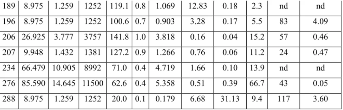
(3b) Table 2 – Results of the hydrological and weathering modelling approaches. Symbols: NR –
identification code of the spring site; A, V and L – associated watershed area, topographic volume and length of talwegs; Dz, Vz and δ – average depth of spring water circulation,
volume of water interacting with percolating spring water and ratio between Vz and V; K and
ne – hydraulic conductivity and effective porosity of the fractured media; t – groundwater
travel time (equated to the mean turnover time); [Pl] and WPl – moles of plagioclase dissolved
in the process of weathering and concomitant weathering rates.
A x105 V x108 L D z Vz x108 K x10-8 t [Pl] WPl x10-15 NR m2 m3 m m δ m3 m/s ne x10 -2 y μmol/L mol/m2.s 4 8.975 1.259 1252 141.4 1.0 1.269 0.66 0.21 17.0 139 0.91 9 8.975 1.259 1252 138.4 1.0 1.242 0.73 0.11 9.5 nd nd 11 17.950 2.518 2504 101.3 0.7 1.818 1.55 0.03 3.1 146 19.55 16 8.975 1.259 1252 97.7 0.7 0.877 1.16 0.17 18.1 242 2.20 18 35.166 5.335 4833 129.6 0.9 4.558 0.49 0.01 1.8 82 20.16 27 10.282 1.492 1425 101.6 0.7 1.044 1.94 0.02 1.6 28 11.46 34 18.942 3.205 2546 108.2 0.6 2.050 0.55 0.01 3.2 53 7.28 58 14.677 2.329 1998 123.6 0.8 1.815 0.64 0.02 4.0 38 3.91 61 21.779 3.816 2907 72.8 0.4 1.586 1.29 0.02 3.9 52 7.16 112 9.207 1.300 1283 78.1 0.6 0.719 0.36 0.02 4.9 nd nd 123 17.950 2.518 2504 26.3 0.2 0.472 30.76 0.69 10.1 nd nd 136 33.401 5.649 4496 70.2 0.4 2.344 0.75 0.03 9.1 88 3.26 143 29.996 4.787 4079 77.0 0.5 2.311 4.06 0.09 8.1 58 2.96 144 8.975 1.259 1252 89.1 0.6 0.800 5.54 0.06 2.8 nd nd 148 8.975 1.259 1252 89.2 0.6 0.801 28.18 0.27 4.4 nd nd 161 48.205 8.012 6509 28.9 0.2 1.391 8.76 0.08 4.2 127 19.22 174 19.763 2.844 2744 94.9 0.7 1.875 2.19 0.06 5.1 111 7.97 180 17.950 2.518 2504 99.0 0.7 1.777 1.37 0.07 4.8 70 4.07
189 8.975 1.259 1252 119.1 0.8 1.069 12.83 0.18 2.3 nd nd 196 8.975 1.259 1252 100.6 0.7 0.903 3.28 0.17 5.5 83 4.09 206 26.925 3.777 3757 141.8 1.0 3.818 0.16 0.04 15.2 57 0.46 207 9.948 1.432 1381 127.2 0.9 1.266 0.76 0.06 11.2 24 0.47 234 66.479 10.905 8992 71.0 0.4 4.719 1.66 0.10 13.9 nd nd 276 85.590 14.645 11500 62.6 0.4 5.358 0.51 0.39 66.7 43 0.05 288 8.975 1.259 1252 20.0 0.1 0.179 6.68 31.13 9.4 117 3.60
The calculated values of Dz (Table 2) range from a minimum of 20 to a maximum of 142 m,
being on average 92±34 m. Comparative to the average topographic thicknesses (V/A = 150±12 m) they represent solely a fraction δ = 63±25 %. In further calculations using the volume of groundwater involved in weathering reactions (Vz), this volume will be defined in
keeping with these results, i.e.:
Vz = δV (4) 87Sr/86Sr = 0,0003621D med+ 0,7100076 R² = 0.99 87Sr/86Sr = 0,0001527D med+ 0,7100076 R² = 0,79 0.705 0.710 0.715 0.720 0.725 0.730 0.735 0.740 0.745 0.750 0 20 40 60 80 100 120 87Sr / 86Sr Dmed(m) P = 1500 mm/y P = 1150 mm/y
Figure 4 – Correlations between the 87Sr/86Sr ratios and D med.
6. Aquifer Formation Constants and Groundwater Travel Times
The estimation of hydraulic conductivities (K, m/y) and effective porosities (ne,
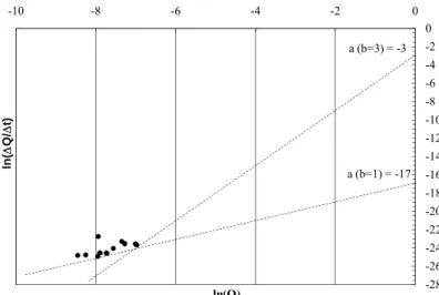
dimensionless) employed the Brutsaert method (Brutsaert and Lopez, 1998). According to this method, in a graphical plot of discharge rate (Q, m3/s) and time (t, s) measurements – ln(ΔQ/Δt) vs. ln(Q) – the lower envelope to the scatter points is represented by two straight lines, one of slope b =1 and the other of slope b = 3, with intercept-y values (a1, a3) related to
K and ne as follows: ⎟ ⎟ ⎠ ⎞ ⎜ ⎜ ⎝ ⎛ = 2 2 3 1 3 57 0 L V A a a K z . (5a)
3 1 98 1 a a V n z e . = (5b)
The method is illustrated in Figure 5 for spring site nr 144. For this station, K = 5.54×10⁻⁸ m/s and ne = 6.0×10⁻², on average K = (4.7±7.9)×10–8 m/s and ne = (1.4±6.1)×10–2 (Table 2).
These values are representative of fractured rock hydraulic conductivities and effective porosities. The discharge rate measurements on which the calculations of K and ne are
standing are presented elsewhere.
The concept of hydraulic turnover time (McGuire and McDonnell, 2006) was used to estimate the mean travel time (t, s) of groundwater within the watershed boundaries. This time is the ratio of the mobile watershed storage (Vzne, m3) to the volumetric flow rate (Vr, m3 in one
year): r e z V n V t= (6)
For station 144, t = 2.8 y, on average 9.6±12.6 y (Table 2).
7. Weathering Model
It was assumed that, in the process of chemical weathering, plagioclase and biotite are the major contributors to the chemistry of springs. The conceptual mole-balance model (SiB algorithm of Pacheco and Van der Weijden, 1996, Pacheco et al., 1999) set the weathering of plagioclase into mixtures of kaolinite and gibbsite because rainfall in the area is always higher than 1000 mm/y (Martins et al., 1995; Van der Weijden and Pacheco, 2006), and set the weathering of biotite into mixtures of kaolinite and vermiculite. The results relative to plagioclase mole fractions ([Pl], mol/L) are depicted in Table 2.
-28 -26 -24 -22 -20 -18 -16 -14 -12 -10 -8 -6 -4 -2 0 -10 -8 -6 -4 -2 0 ln( Δ Q/ Δ t) ln(Q) a (b=3) = -3 a (b=1) = -17
8. Plagioclase Weathering Rates and the Duration of Weathering Episodes
Plagioclase weathering rates can be determined with the formula (Pacheco and Van der Weijden, 2009): WPl = [Pl] 2× t ×αPl 12μwK ρwgne (7)
where αPl is the proportion of plagioclase in the rocks, ρw(kg/m3) and μw(kg/s·m) are the
specific weight and dynamic viscosity of water (at T = 15ºC, ρw = 999.1 kg/m3, and μw = 1.14
× 10–3 kg/s·m), g (9.81 m/s2) is the acceleration of gravity. Considering that most spring
waters circulate in granite environment, it was assumed that αPl = 0.35. Rates calculated by Equation 7 for all the springs are listed in Table 2 (last column), being on average (5.7±5.6) × 10–15 mol/m2·s.
White and Brantley (2003) investigated the effect of time on the weathering of plagioclase and concluded that concomitant rates decrease according to a power function of the duration of weathering. This function is identified in Figure 6 as “average trend”. However, laboratory experiments reveal that at initial stages of weathering plagioclase dissolution rates fit to a steeper power function indentified as “initial trend”.
The duration of weathering is unknown within the springs’ watersheds. However, it is certain that each spring water sample is one after many other fluid packets that already flew across the local granite and metassediment aquifers. It is striking then how plagioclase weathering rates calculated for the springs (filled circles) fit to the initial trend. Apparently, notwithstanding weathering is continuously happening within the watershed, meaning that the duration of weathering is larger than the groundwater travel time used to produce the plot of the springs, every new fluid packet seems to invade unweathered sectors of the massif and therefore to represent a “initial” stage of weathering.
In most studies, the duration of weathering episodes comprises the time required by water to convert a fresh rock into a soil or saprolite, and is most commonly determined from distributions of cosmogenic isotopes leading to ages up to 3.02×10⁻⁶ y (White and Brantley, 2003). However, the process of soil and saprolite formation involves solely a small portion of the watershed volume. An attempt to extend the isotopic approach to the scale of a watershed would undoubtedly result in much longer times. The differences in scale resulting from studies focused at the soil profile or at the watershed might after all explain why the filled circles follow the steeper trend line. Eventually, this is because weathering in the spring watersheds although is occurring over geological time scales, the episodes are just starting given the awesome volumes of rock that have to be broken apart.
0.0001 0.001 0.01 0.1 1 10 100 0.001 0.01 0.1 1 10 100 1000 10000 100000 1000000 W ea the ri ng r a te -W Pl (x10 -1 3m o l/m 2.s ) Time - t (yr) Initial trend Average trend
Literature results (laboratory) Literature results (field) Vila Pouca de Aguiar springs
WPl= 3,47x10⁻¹³t-0,56
R2= 0,89
WPl= 1,28x10⁻¹³t-1,57
R2= 0,64
Figure 6 – Plagioclase weathering rates and the duration of weathering episodes. For the literature results and trends, time is the duration of weathering, for the Vila Pouca de Aguiar springs time is the travel time.
References
Brutsaert, W., Lopez, J.P. (1998). Basin-scale geohydrologic drought flow features of riparian aquifers of the southern Great Plains. Water Resour. Res. 30: 2759–2763.
ESRI (2007). ArcHydro tools - tutorial, version 1.2, for ArcInfo 9.2. ESRI, Redlands, USA, 110pp.
Horton, R. E. 1945. Erosional development of streams and their drainage basins: hydrophysical approach to quantitative morphology. Geological Society of America Bulletin 56:275-370.
McGuire, K.J., McDonnell, J.J. (2006). A review and evaluation of catchment transit time modelling. J. Hydrol. 330: 543-563.
Martins, A.A.A., Madeira, M.V., Refega, A.A.G. (1995). Influence of rainfall on properties of soils developed on granite in Portugal. Arid Soil Research and Rehabilitation, 9: 353–366.
Pacheco, F.A.L. (1995) Interacção Água-Rocha em Unidades do Grupo Peritransmontano (Serra da
Padrela-Vila Pouca de Aguiar). Tese de Mestrado, Universidade de Coimbra, Coimbra, 123p.
Pacheco, F.A.L., Van der Weijden, C.H. (1996). Contributions of water-rock interactions to the composition of ground water in areas with sizeable anthropogenic input. A case study of the waters of the Fundão area, central Portugal. Water Resour. Res. 32: 3553–3570.
Pacheco, F.A.L., & Van der Weijden, C.H., (2009, submetido). Hydrologic and kinetic modeling of plagioclase
weathering rates in the Vouga basin (Portugal): reconciling field and laboratory rates. Geophysics,
Geochemistry and Geosystems (G3).
Pacheco, F.A.L., Sousa Oliveira, A., Van der Weijden, A.J., Van der Weijden, C.H. (1999). Weathering, biomass production and ground water chemistry in an area of dominant anthropogenic influence, the Chaves-Vila Pouca de Aguiar region, north of Portugal. Water Air Soil Poll. 115: 481–512.
Strahler, A. N. (1957). Quantitative Analysis of Watershed Geomorphology. Transactions of the American
Geophysical Union 8 (6): 913–920.
Van der Weijden, C.H., Pacheco, F.A.L. (2006). Hydrogeochemistry in the Vouga River basin (central Portugal): pollution and chemical weathering. Appl. Geochem. 21: 580–613.
White, A.F., Brantley, S.L. (2003). The effect of time on the weathering of silicate minerals: why do weathering rates differ in the laboratory and field? Chem. Geol. 202: 479–506.